Adaptive Feedforward Control of a Pressure Compensated Differential Cylinder

Abstract

This paper presents the design, simulation and experimental verification of adaptive feedforward motion control for a hydraulic differential cylinder. The proposed solution is implemented on a hydraulic loader crane. Based on common adaptation methods, a typical electro-hydraulic motion control system has been extended with a novel adaptive feedforward controller that has two separate feedforward states, i.e, one for each direction of motion. Simulations show convergence of the feedforward states, as well as 23% reduction in root mean square (RMS) cylinder position error compared to a fixed gain feedforward controller. The experiments show an even more pronounced advantage of the proposed controller, with an 80% reduction in RMS cylinder position error, and that the separate feedforward states are able to adapt to model uncertainties in both directions of motion.

1. Introduction

For hydraulically actuated systems such as cranes, the hydraulic cylinder is the most common actuator since it can provide a linear motion with, generally speaking, a large force to volume ratio, a high efficiency and at a modest price. For systems which require a cylinder force in both directions, a double acting cylinder is needed, and the differential cylinder is an obvious choice due to its low cost and simple design. The main disadvantage is the difference in effective hydraulic area which leads to a jump in both velocity and force gain when changing sign of direction, i.e., around zero velocity.

For many hydraulic systems, the pressure compensated directional control valve is a practical choice due to the fact that it provides load independent flow control of the actuators. The pressure compensator senses the load pressure, and adjusts the pressure drop over the directional control valve to give a load independent flow. Since the velocity of the actuator is proportional to the hydraulic flow through the valve, this translates to load independent velocity control. For manually operated systems, the velocity control makes it easy for an operator to control systems that are subjected to large variations in external load.

For closed loop control systems, the load independent velocity control can be utilized in a control system using feedforward [1]. In this case, both a position reference and a velocity reference are generated in the control system. An example of a typical closed loop electro-hydraulic motion control system with feedforward is shown in Figure 1. The feedback controller uses the position reference and the measured cylinder position, whereas the feedforward controller uses the velocity reference. The pressure compensator is connected to a supply line which is shared with other actuators. The red dashed lines show the hydraulic pilot lines for the counterbalance valve and the pressure compensator.

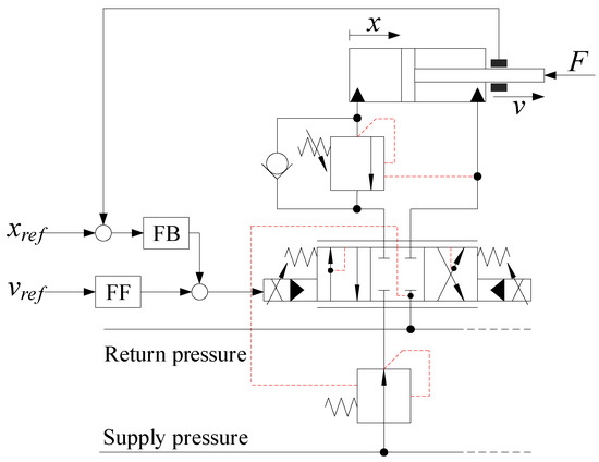
Figure 1. Electro-hydraulic motion control system with feedforward.

It should be noted that feedforward control cannot be used alone. A feedback controller is also needed to help track the position reference, to eliminate steady state position error, and to counteract any drift. Normally the feedforward gain is based on system components, and is defined as the ratio of valve opening to actuator velocity. With this in mind, it follows that modeling errors and model uncertainties, in addition to external disturbances and system dynamics, may yield sub-optimal performance with a fixed feedforward gain.

This paper focuses on modeling and motion control of a hydraulic loader crane with pressure compensated differential cylinders. An adaptive feedforward controller is investigated to improve performance of the motion control system. Two different approaches to feedforward control have been implemented, the first is based on the MIT-rule [2], and the second is based on the sign-sign algorithm [3].

2. Background and Method

Adaptive systems have long been used for system identification and parameter estimation. One of the first methods is described in [4]. Another common method is the least mean squares algorithm, which was developed in [5]. An example of this is shown in Equations (1)–(3). Given the linear system:

$$\begin{array}{cc}\hfill Y& \hfill ={\theta }^T·X\hfill \end{array}$$

(1)

$$\begin{array}{cc}\hfill E& \hfill =Y-{\widehat{\theta }}^T·X\hfill \end{array}$$

(2)

$$\begin{array}{cc}\hfill \dot{\widehat{\theta }}& \hfill =\gamma ·X·E^T\hfill \end{array}$$

(3)

where

• Y = system output;
• $\theta$ = system parameters;
• X = system input;
• E = estimation error;
• $\widehat{\theta }$ = estimated parameters;
• $\gamma$ = adaptation gain, constant.

The estimated parameters will converge towards the system parameters. The idea of using the sign function in the adaptive law comes from the sign-sign least mean squares algorithm, and was first introduced by [3]. Equation (3) then becomes:

$$\begin{array}{cc}\hfill \dot{\widehat{\theta }}& \hfill =\gamma ·sign\left(X\right)·sign\left(E^T\right)\hfill \end{array}$$

(4)

By taking the sign of the estimation error and system input, the adaptation becomes insensitive to the magnitudes of E and X, and as such only the adaptation gain $\gamma$ sets the adaptation speed.

The MIT rule is also used for adaptive control, and is described in [2]. A typical application is model reference adaptive control, shown in Figure 2. Based on the model output $y_m$, an additional control output $\widehat{u}$ is multiplied with the command signal $u_c$ to shape the plant output y. The equations for the model reference adaptive control is shown in Equations (5) and (6).

$$\begin{array}{cc}\hfill \dot{\widehat{u}}& \hfill =-\gamma ·y_m·(y-y_m)\hfill \end{array}$$

(5)

$$\begin{array}{cc}\hfill u& \hfill =u_c·\widehat{u}\hfill \end{array}$$

(6)

where

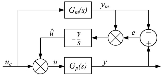
Figure 2. Model reference adaptive control based on MIT-rule.

• u = control output;
• $\widehat{u}$ = adaptive control output;
• $u_c$ = command signal;
• $y_m$ = model output;
• y = plant output.

Early work in adaptive control can be found in [6,7,8,9,10]. Other work on adaptive control include [11] which investigates adaptive feedback and feedforward control of robot manipulators, Reference [12] which models and implements adaptive control of a flexible arm, and [13] which uses model reference adaptive control on linear time-varying plants. Adaptive fuzzy sliding mode control is investigated and implemented on an inverted pendulum in [14].

Newer applications of adaptive control systems include adaptive friction compensation with an adaptive velocity estimator to compensate for the estimated non-linear friction force [15]. In [16], a fuzzy model reference adaptive control of an active magnetic bearing for a milling process is investigated to reduce the milling dynamics. Adaptive integral robust control of an electro-hydraulic servo system is investigated in [17], using parameter estimation and integral control to compensate for disturbances and plant uncertainties. Adaptive control of quadrotors is investigated in [18], which uses an cerebellar model arithmetic computer to adapt to model uncertainties and disturbances. In [19], adaptive control based on least-mean-fourth is implemented for a three-phase grid connected solar system, which is able to provide load balancing and power factor correction.

As for motion control of hydraulic systems, different approaches have previously been investigated, including vector control [20], pressure control [21,22], force control [23,24], and feedforward control [25]. To the knowledge of the authors, adaptive feedforward motion control of hydraulic cylinders has not previously been investigated, and this paper will focus on this novel concept.

In this paper, two adaptive controllers have been tested on a hydraulic differential cylinder and compared to a fixed gain feedforward controller. Based on a typical fixed gain feedforward controller, an adaptive controller can be made by extending it with the MIT rule. An illustration of a control system with feedforward with fixed gain is shown in Figure 3.

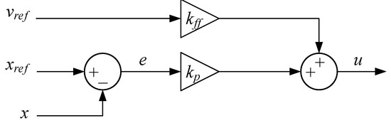
Figure 3. Feedforward with fixed gain.

Defining the position error e as the position reference $x_{ref}$ minus the measured position x, the control output for this control system is given in Equation (7)

$$\begin{array}{cc}\hfill u& \hfill =k_p·e+k_{ff}·v_{ref}\hfill \end{array}$$

(7)

where

• u = controller output;
• $k_p$ = proportional gain;
• e = position error;
• $k_{ff}$ = feedforward gain;
• $v_{ref}$ = velocity reference.

Extending the traditional feedforward controller into an adaptive feedforward controller is done by replacing the fixed feedforward gain with the MIT-rule. An illustration of the adaptive feedforward scheme is shown in Figure 4.

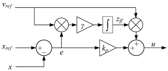
Figure 4. MIT-rule adaptive feedforward.

The MIT-rule adaptive feedforward controller uses the position error, the velocity reference, and the constant $\gamma$ to update the feedforward gain. The update law and the control output for this adaptive control system is then given in Equations (8) and (9).

$$\begin{array}{cc}\hfill {\dot{z}}_{ff}& \hfill =\gamma ·v_{ref}·e\hfill \end{array}$$

(8)

$$\begin{array}{cc}\hfill u& \hfill =k_p·e+z_{ff}·v_{ref}\hfill \end{array}$$

(9)

where

• $\gamma$ = adaptation gain;
• $z_{ff}$ = feedforward gain.

Extending this controller to use sign-sign is then straightforward. An illustration of the sign-sign adaptive feedforward scheme is shown in Figure 5.

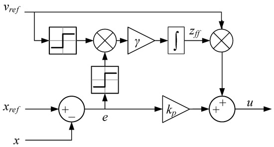
Figure 5. Sign-sign adaptive feedforward.

The update law and the control output for this adaptive control system is shown in Equations (10) and (11).

$$\begin{array}{cc}\hfill {\dot{z}}_{ff}& \hfill =\gamma ·sign\left(v_{ref}\right)·sign\left(e\right)\hfill \end{array}$$

(10)

$$\begin{array}{cc}\hfill u& \hfill =k_p·e+z_{ff}·v_{ref}\hfill \end{array}$$

(11)

It should be noted that the sign function can produce unnecessary chattering when the input is oscillating around zero, due to the inherent discontinuity. Therefore the sign function has been replaced with the tanh function, shown in Equation (12).

$$\begin{array}{cc}\hfill sign\left(e\right)& \hfill \approx tanh(k·e)\hfill \end{array}$$

(12)

This gives a smooth output when the input is oscillating around zero. Increasing the parameter k gives a sharper rise and a closer approximation to $sign\left(e\right)$. Another advantage of using tanh is that the adaptation stops when the position error is zero. The parameter k has been set to $k=100{\mathrm{m}}^{-1}$ and $k=100\mathrm{s}·{\mathrm{m}}^{-1}$ for the position error and velocity reference, respectively.

3. Considered System

In this paper an 2020K4 loader crane made by HMF Group A/S, Højbjerg, Denmark has been used for experiments. An illustration of the crane is shown in Figure 6. This crane has two hydraulic differential cylinders: the main cylinder, and the knuckle cylinder. For this paper, the knuckle cylinder has been used for simulation and experiments, since it can experience both resistive and assistive loads in both directions of motion, equivalent to four quadrant operation. The relevant data for the knuckle cylinder is shown in Table 1, and the data for the knuckle boom is given in Figure 7 and Table 2.

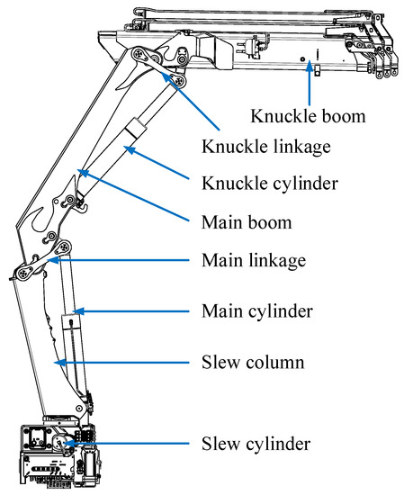
Figure 6. Illustration of the HMF 2020K4 loader crane.

Table 1. Knuckle cylinder data.

Name	Parameter	Value
Piston diameter	$D_p$	0.15 m
Piston area	A	0.0177 m${}^2$
Rod diameter	$D_r$	0.1 m
Annulus area	$A_a$	0.0098 m${}^2$
Piston area ratio	$\varphi =\frac{A_a}{A}$	0.5556
Valve maximum flow	$Q_{max}$	40 L/min

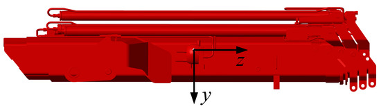
Figure 7. Knuckle boom center of mass.

Table 2. Knuckle boom data.

Name	Parameter	Value
Mass	$m_k$	851.972 kg
Inertia matrix	$I_k$	$\left[\begin{array}{ccc}579.552& 8.74629& 11.5456\\ 8.74629& 573.285& 0.174433\\ 11.5456& 0.174433& 32.2491\end{array}\right]$ kg·m${}^2$

Each actuator is controlled via a pressure compensated proportional directional control valve which ensures load independent flow control of the actuators. Counterbalance valves made by Oil Control S.p.A, Modena, Italy are also used for load holding, assisting in lowering of the booms, and pressure relief of pressure surges. An illustration of the hydraulic system for the knuckle cylinder is shown in Figure 8.

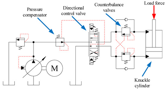
Figure 8. Hydraulic system for the knuckle cylinder.

The control system is implemented on a CompactRIO 9075 controller made by National Instruments, Austin, TX, USA. The CompactRIO contains the reference generator and feedforward motion controllers. The block diagram of the connections is shown in Figure 9.

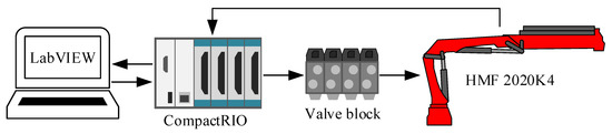
Figure 9. Connection between the crane and CompactRIO controller.

The CompactRIO communicates with a PC, sends control signals to the valves, and reads the sensors on the crane.

4. Modelling

A dynamic model of the crane has been made in Simscape™ by MathWorks®, Natick, MA, USA. 3D computer-aided design (CAD) models have been imported into the model using the Multibody library. The hydraulic circuit has been made using the hydraulic library of Simscape™. A picture of the CAD model is shown in Figure 10.

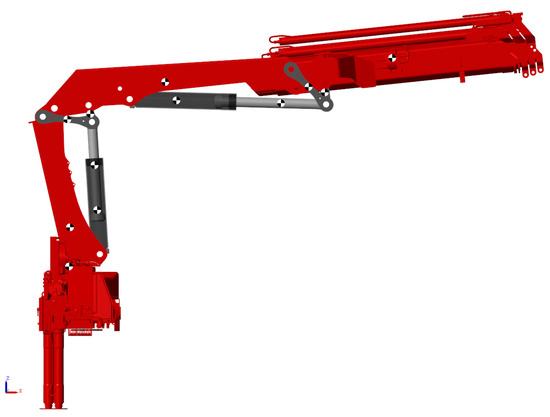
Figure 10. 3D view of the simulation model of the HMF 2020K4 in Simscape.

In the configuration shown in Figure 10, the knuckle cylinder experiences both resistive and assistive loads in both directions of motion when retracting fully, and extending back out again. The knuckle cylinder is controlled by a pressure compensated directional control valve, shown in Figure 11.

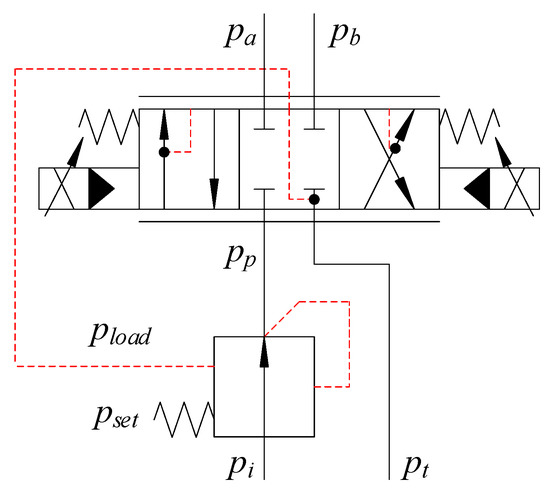
Figure 11. Hydraulic pressure compensated directional control valve for the knuckle cylinder.

The pressure compensator ensures that there is a constant pressure drop over the directional control valve, which gives a load independent flow. The governing equations of the pressure compensator are given in Equations (13)–(15).

$$\begin{array}{cc}\hfill u_{pc}& \hfill =\frac{p_{set}+p_{load}-p_p}{\Delta p}\hfill \end{array}$$

(13)

$$\begin{array}{cc}\hfill p_{load}& \hfill =\left\{\begin{array}{cc}\hfill p_a\hfill & \hfill \mathrm{if}{u}_{spool}\ge 0\hfill \\ \hfill p_b\hfill & \hfill \mathrm{otherwise}\hfill \end{array}\right.\hfill \end{array}$$

(14)

$$\begin{array}{cc}\hfill Q_{pc}& \hfill =k_{pc}·u_{pc}·\sqrt{p_i-p_p}\hfill \end{array}$$

(15)

where

• $u_{pc}$ = opening of compensator, $0\le u_{pc}\le 1$
• $p_p$ = compensated pressure at port p;
• $\Delta p$ = pressure difference between fully closed and fully open;
• $p_a$ = pressure at port a;
• $p_b$ = pressure at port b;
• $p_t$ = tank pressure;
• $p_{set}$ = spring pressure setting;
• $p_{load}$ = load pressure;
• $u_{spool}$ = position of the main spool, $-1\le u_{spool}\le 1$;
• $Q_{pc}$ = flow in pressure compensator;
• $k_{pc}$ = flow gain of compensator;
• $p_i$ = compensator inlet pressure.

The steady state of $p_p$ is then given by Equation (16).

$$\begin{array}{cc}\hfill p_p& \hfill =p_{load}+p_{set}\hfill \end{array}$$

(16)

The sensing of the load pressures $p_a$ and $p_b$ ensures that the pressure drop over the directional control valve always equals $p_{set}$, and that the flow is load independent. This is shown in the orifice equation in Equation (17).

$$\begin{array}{cc}\hfill Q& \hfill =C_d·A_d·u_{spool}·\sqrt{\frac{2}{\rho }·(p_p-p_{load})}\hfill \\ \hfill & \hfill =C_d·A_d·u_{spool}·\sqrt{\frac{2}{\rho }·p_{set}}\hfill \\ \hfill & \hfill =Q_{max}·u_{spool}\hfill \end{array}$$

(17)

where

• Q = flow in the valve;
• $C_d$ = discharge coefficient;
• $A_d$ = maximum discharge area;
• $\rho$ = mass density;
• $Q_{max}$ = maximum valve flow;

Double counterbalance valves are used on the knuckle cylinder. An illustration of the counterbalance valves is shown in Figure 12.

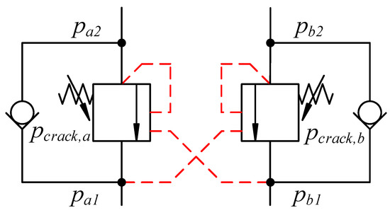
Figure 12. Double counterbalance valve.

The unitless openings of the counterbalance valves are calculated in Equations (18) and (19).

$$\begin{array}{cc}\hfill u_a& \hfill =\frac{p_{a2}+\psi ·p_{b1}-p_{crack,a}}{\Delta p}\hfill \end{array}$$

(18)

$$\begin{array}{cc}\hfill u_b& \hfill =\frac{p_{b2}+\psi ·p_{a1}-p_{crack,b}}{\Delta p}\hfill \end{array}$$

(19)

where

• $u_a$ = opening of valve a, $0\le u_a\le 1$;
• $u_b$ = opening of valve b, $0\le u_b\le 1$;
• $p_{a1}$ = pressure at valve a input side;
• $p_{a2}$ = pressure at valve a actuator side;
• $p_{b1}$ = pressure at valve b input side;
• $p_{b2}$ = pressure at valve b actuator side;
• $p_{crack,a}$ = crack pressure of valve a;
• $p_{crack,b}$ = crack pressure of valve b;
• $\psi$ = pilot area ratio;
• $\Delta p$ = pressure difference between fully closed and fully open.

When $u_a$ and $u_b$ are 0, the valves are closed. When they are 1, the valves are fully open. During assistive loads the valves tend to be somewhere between 0 and 1, meaning that they are throttling the flow. The dynamics of the valves are included as a time constant, since the valves have a finite bandwidth.

5. Adaptive Control Design

Since the actuator is a hydraulic differential cylinder, two separate states $z_{ff}^{+}$ and $z_{ff}^{-}$ are used for out-stroke and in-stroke motion to handle model uncertainties both directions of motion. Consequently, both the feedforward control output and the update law for the two gains are only active during out-stroke or in-stroke motion respectively. To handle this, some switching logic is introduced based on the sign of the velocity reference. The block diagram for the differential MIT-rule adaptive feedforward is shown in Figure 13.

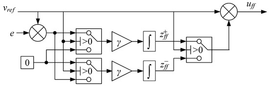
Figure 13. Differential MIT-rule adaptive feedforward.

The governing equations for the differential MIT-rule adaptive feedforward are shown in Equations (20)–(23).

$$\begin{array}{cc}\hfill {\dot{z}}_{ff}^{+}& \hfill =\left\{\begin{array}{cc}\hfill \gamma ·v_{ref}·e,\hfill & \hfill v_{ref}>0\hfill \\ \hfill 0,\hfill & \hfill \mathrm{otherwise}\hfill \end{array}\right.\hfill \end{array}$$

(20)

$$\begin{array}{cc}\hfill {\dot{z}}_{ff}^{-}& \hfill =\left\{\begin{array}{cc}\hfill 0,\hfill & \hfill v_{ref}>0\hfill \\ \hfill \gamma ·v_{ref}·e,\hfill & \hfill \mathrm{otherwise}\hfill \end{array}\right.\hfill \end{array}$$

(21)

$$\begin{array}{cc}\hfill u_{ff}& \hfill =\left\{\begin{array}{cc}\hfill z_{ff}^{+}·v_{ref},\hfill & \hfill v_{ref}>0\hfill \\ \hfill z_{ff}^{-}·v_{ref},\hfill & \hfill \mathrm{otherwise}\hfill \end{array}\right.\hfill \end{array}$$

(22)

$$\begin{array}{cc}\hfill u& \hfill =k_p·e+u_{ff}\hfill \end{array}$$

(23)

where

• $z_{ff}^{+}$ = out-stroke feedforward gain;
• $z_{ff}^{-}$ = in-stroke feedforward gain;
• $u_{ff}$ = feedforward controller output.

Extending the controller to sign-sign is straightforward. The block diagram for the differential sign-sign adaptive feedforward is shown in Figure 14.

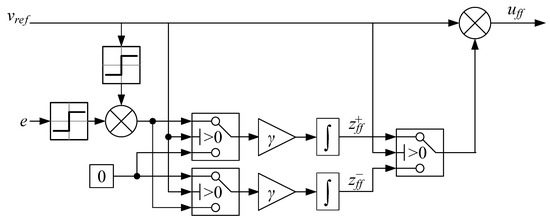
Figure 14. Differential sign-sign adaptive feedforward.

The governing equations for the differential sign-sign adaptive feedforward are shown in Equations (24)–(27).

$$\begin{array}{cc}\hfill {\dot{z}}_{ff}^{+}& \hfill =\left\{\begin{array}{cc}\hfill \gamma ·sign\left(v_{ref}\right)·sign\left(e\right),\hfill & \hfill v_{ref}>0\hfill \\ \hfill 0,\hfill & \hfill \mathrm{otherwise}\hfill \end{array}\right.\hfill \end{array}$$

(24)

$$\begin{array}{cc}\hfill {\dot{z}}_{ff}^{-}& \hfill =\left\{\begin{array}{cc}\hfill 0,\hfill & \hfill v_{ref}>0\hfill \\ \hfill \gamma ·sign\left(v_{ref}\right)·sign\left(e\right),\hfill & \hfill \mathrm{otherwise}\hfill \end{array}\right.\hfill \end{array}$$

(25)

$$\begin{array}{cc}\hfill u_{ff}& \hfill =\left\{\begin{array}{cc}\hfill z_{ff}^{+}·v_{ref},\hfill & \hfill v_{ref}>0\hfill \\ \hfill z_{ff}^{-}·v_{ref},\hfill & \hfill \mathrm{otherwise}\hfill \end{array}\right.\hfill \end{array}$$

(26)

$$\begin{array}{cc}\hfill u& \hfill =k_p·e+u_{ff}\hfill \end{array}$$

(27)

6. Simulation Results

For the simulation, a point-to-point trapezoidal velocity path generator has been used as a reference. The point-to-point path generator has previously been developed in [26]. The path generator operates in actuator space, which eliminates the effects of the non-linearities between the hydraulic cylinder strokes and the joint angles in joint space. A path has been made such that the cylinder experiences both resistive and assistive loads in both directions of motion. The references for position and velocity are shown in Figure 15. The adaptation gain $\gamma$ is different for the two controllers, due to the use of $sign\left(x\right)$, and has been experimentally set to $\gamma =200\mathrm{s}·{\mathrm{m}}^{-3}$ for the MIT-rule feedforward, and $\gamma =0.1{\mathrm{m}}^{-1}$ for the sign-sign feedforward. The unit is adapted accordingly to obtain the correct output.

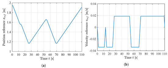
Figure 15. Point-to-point path references for simulation. (a) Position reference; (b) Velocity reference.

The position error for the MIT-rule feedforward simulation is shown in Figure 16. The position error decreases towards a bounded error of $\pm 6$ mm, which is shown with the dashed lines. The RMS error after convergence is 1.6 mm, showing high performance.

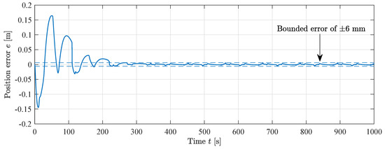
Figure 16. Cylinder position error during MIT-rule feedforward simulation, $\gamma =200\mathrm{s}·{\mathrm{m}}^{-3}$.

The states $z_{ff}$ for the MIT-rule feedforward simulation are shown in Figure 17. The dashed lines show the theoretical values for a fixed feedforward gain. The states converge to values slightly larger than the theoretical ones. This small discrepancy can be attributed to the constant velocity reference and ramped position reference. When moving with a ramp position reference, there will always be a small constant position error without an integrator in the position controller. Having a slightly larger feedforward gain helps reducing this constant position error by giving the cylinder a small velocity boost. Since the position error is measured, the adaptive controller is able to adapt the feedforward gains to minimize the position error.

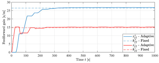
Figure 17. Feedforward states during MIT-rule feedforward simulation, $\gamma =200\mathrm{s}·{\mathrm{m}}^{-3}$.

Figure 18 shows the control signals $u_{ff}$ and $u_{fb}$ from the feedforward and feedback controller, respectively. Given that the total control signal $u=u_{fb}+u_{ff}$, it can be seen that the contribution from the feedforward controller clearly dominates, providing more than 95% at steady state.

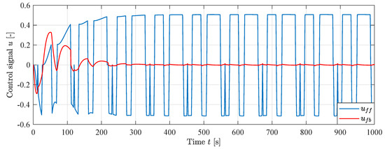
Figure 18. Control signals from feedforward and feedback during simulation, $\gamma =200\mathrm{s}·{\mathrm{m}}^{-3}$.

The position error for the sign-sign feedforward simulation is shown in Figure 19. The same bounded error of $\pm 6$ mm is shown with the dashed lines. The RMS error after convergence is 2.1 mm.

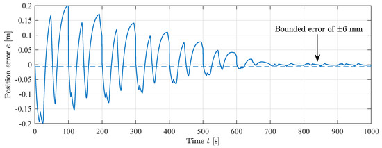
Figure 19. Cylinder position error during sign-sign feedforward simulation, $\gamma =0.1{\mathrm{m}}^{-1}$.

The states $z_{ff}$ for the sign-sign feedforward simulation are shown in Figure 20. The dashed lines show the theoretical values for a fixed feedforward gain. The same results can be seen here as with the MIT-rule, the states converge to values slightly larger than the theoretical ones, although convergence is slower with 700 s compared to 400 s.

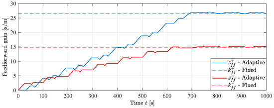
Figure 20. Feedforward states during sign-sign feedforward simulation, $\gamma =0.1{\mathrm{m}}^{-1}$.

To show the difference in performance between the fixed gain controller and the adaptive controllers, a simulation with fixed gain feedforward has been made and compared with the MIT-rule feedforward at a simulation time where the states $z_{ff}$ have converged, at $t=800$ s. This is shown in Figure 21. It can be seen that the position error for the MIT-rule feedforward is lower compared to the fixed gain feedforward, showing that the MIT-rule feedforward controller outperforms the fixed gain controller even with an ideal model with correlation between cylinder velocity and feedforward gain.

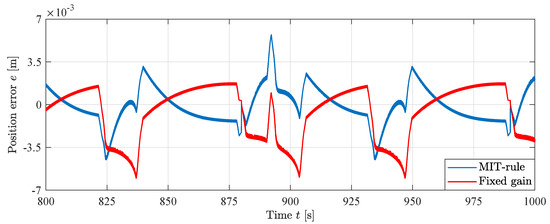
Figure 21. Position error comparison between MIT-rule and fixed gain feedforward in simulation.

The RMS position error for each controller after convergence of the states $z_{ff}$ is shown in Table 3. Even though the fixed gain feedforward is based on an ideal model, the MIT-rule adaptive feedforward controller yields better position tracking with a 23% decrease in RMS position error. This shows the improved performance of the adaptive controller.

Table 3. Comparison of RMS position error after convergence in simulation.

	MIT-Rule	Sign-Sign	Fixed Gain
RMS error	1.6 mm	2.1 mm	2.1 mm

7. Experimental Results

The three controllers have been implemented on the CompactRIO controller in the laboratory. The control laws are implemented in discrete-time based on backward euler integration. A picture of the HMF 2020K4 loader crane in the laboratory is shown in Figure 22. The figure shows the crane in the starting position. During motion the knuckle boom is folded down.

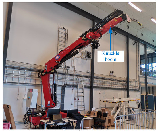
Figure 22. HMF 2020K4 loader crane in the laboratory.

There is some deadband in the valves on the HMF 2020K4 loader crane, and therefore deadband compensation has been implemented for the laboratory experiments. The identified deadbands for the knuckle boom valve are shown in Table 4.

Table 4. Identified deadbands for the knuckle boom valve.

Name	Parameter	Value
Out-stroke deadband	$u^{+}$	0.21
In-stroke deadband	$u^{-}$	−0.31

The equation for the deadband compensation is shown in Equation (28). By adding a small deadband $\tilde{u}$, it is ensured that the valve will be able to stay closed when no movement is needed.

$$\begin{array}{cc}\hfill \widehat{u}=& \hfill \left\{\begin{array}{cc}\hfill u^{+}+(1-u^{+})·u,\hfill & \hfill u>\tilde{u}\hfill \\ \hfill u^{-}+(1+u^{-})·u,\hfill & \hfill u<-\tilde{u}\hfill \\ \hfill 0,\hfill & \hfill \mathrm{otherwise}\hfill \end{array}\right.\hfill \end{array}$$

(28)

where

• $\widehat{u}$ = compensated control signal;
• u = control signal;
• $u^{+}$ = Out-stroke deadband;
• $u^{-}$ = In-stroke deadband;
• $\tilde{u}$ = desired deadband, 0.001.

The cylinder is running with a point-to-point path in actuator space equal to the simulations. The position error for the MIT-rule feedforward is shown in Figure 23. It is shown that the position error decreases towards a bounded error of ±14 mm. The RMS error after convergence is 5.2 mm. The convergence of the position error is similar to the simulations, showing that the proposed adaptive controller is feasible in a real world scenario, albeit with slightly larger position error.

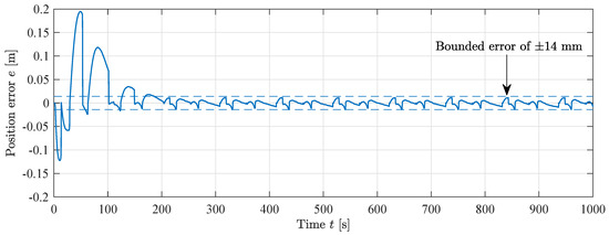
Figure 23. Position error during MIT-rule feedforward experiment, $\gamma =200\mathrm{s}·{\mathrm{m}}^{-3}$.

The states $z_{ff}$ for the MIT-rule feedforward experiment are shown in Figure 24. The dashed lines show the theoretical values for a fixed feedforward gain. The states converge to values that differ from the theoretical ones. The state $z_{ff}^{+}$ is higher than the theoretical, while the state $z_{ff}^{-}$ is lower. This means that there exist some model uncertainties that the controller is able to adapt to. In addition, the ratio of the feedforward gains differs from the cylinder area ratio $\varphi$, i. e. $\frac{z_{ff}^{-}}{z_{ff}^{+}}\ne \frac{A_a}{A}$, showing the importance of using two separate feedforward states. Since the two states are not mathematically linked by the cylinder area ratio $\varphi$, they are able to converge to values that minimizes position error in both directions of motion regardless of their ratio. This would not be possible if the traditional MIT-rule with a single state was used.

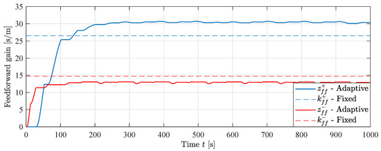
Figure 24. Feedforward states during MIT-rule feedforward experiment, $\gamma =200\mathrm{s}·{\mathrm{m}}^{-3}$.

The position error for the sign-sign feedforward is shown in Figure 25. The same bounded error of ±14 mm is shown. The RMS error after convergence is 5.3 mm.

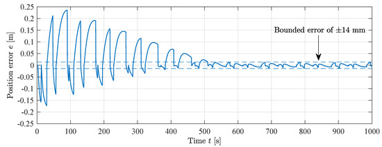
Figure 25. Position error during sign-sign feedforward experiment, $\gamma =0.1{\mathrm{m}}^{-1}$.

The states $z_{ff}$ for the sign-sign feedforward experiment are shown in Figure 26. Similar results can be seen here as with the MIT-rule, the states converge to values that differ from the theoretical ones. The dashed lines show the theoretical values for a fixed feedforward gain. The convergence is slower than the MIT-rule feedforward, and even though convergence speed is not critical, it may be a minor disadvantage compared to the MIT-rule feedforward.

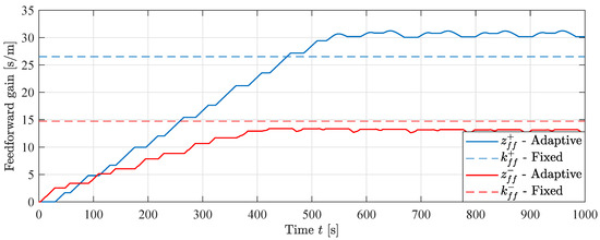
Figure 26. Feedforward states during sign-sign feedforward experiment, $\gamma =0.1{\mathrm{m}}^{-1}$.

The same comparison as in the simulations is made in the laboratory. An experiment with fixed gain feedforward has been made and compared with the MIT-rule feedforward at a time where the states $z_{ff}$ have converged, at $t=800$ s. Figure 27 shows the difference in performance between the fixed gain controller and the adaptive controller, where the position error for the MIT-rule feedforward is significantly lower compared to the fixed gain feedforward.

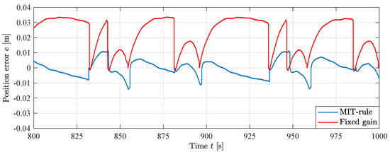
Figure 27. Position error with fixed and adaptive gains.

The RMS position error for each controller after convergence of the states $z_{ff}$ is shown in Table 5. The two adaptive feedforward controllers yield excellent performance with an 80% decrease in RMS position error.

Table 5. Comparison of RMS position error after convergence in experiment.

	MIT-Rule	Sign-Sign	Fixed Gain
RMS error	5.2 mm	5.3 mm	24.9 mm

In general, the RMS position errors are slightly larger than in the simulations, but this is expected and can be attributed to the unmodeled flexibility of the crane, and other unmodeled dynamics. However, the advantage of the adaptive feedforward controller is clear. The independent adaptation of the out-stroke and in-stroke states $z_{ff}^{+}$ and $z_{ff}^{-}$ provides significantly increased performance on a physical system with model uncertainties.

8. Conclusions

In this paper two adaptive feedforward motion controllers are designed, simulated, evaluated, implemented and experimentally verified on a loader crane with hydraulic differential cylinders. The controllers are based on common and proven adaptation methods to extend a typical electro-hydraulic motion control system into a novel adaptive feedforward motion controller. One of the challenges associated with a differential cylinder, namely the jump in both velocity and force gain when changing sign of direction, is solved by creating two separate feedforward states for out-stroke and in-stroke motion of the hydraulic differential cylinder, respectively. This separation makes the controller able to adapt to model uncertainties where the ratio between the in-stroke and out-stroke feedforward gains is not equal to the cylinder area ratio $\varphi$. Adaptation of the feedforward states only occurs when the hydraulic cylinder is moving in the direction of motion associated with the feedforward state.

Simulation results show high performance with good position tracking and that the states $z_{ff}$ converge to values slightly higher than the theoretical ones. The cylinder position error is lowest for the MIT-rule controller with an RMS error of 1.6 mm, and shows faster convergence than the sign-sign controller. Compared to a fixed gain feedforward controller, where the gain is equal to the ratio of valve opening to cylinder velocity, the RMS error is reduced by 23%, showing the improved performance of the novel adaptive feedforward controllers.

Experiments in the laboratory show even better results than in the simulations. The adaptive feedforward controllers converge and show good position tracking, while the MIT-rule feedforward converges faster than the sign-sign feedforward. Compared to a fixed gain feedforward, the RMS position error is reduced by 80% to 5.2 mm for the MIT-rule. The results show the feasabillty of the novel adaptive feedforward controllers on a physical system. In addition, the differential structure of the controllers shows its advantage, as the ratio of the feedforward states converges to values different than the cylinder area ratio $\varphi$, showing the excellent performance of the adaptive feedforward controller and its capability of handling model uncertainties in both directions of motion.

Future work may include stability analysis of the adaptive controllers, since the feedforward gains are dependent on feedback of the cylinder position error e. The effects of the adaptation gain $\gamma$ may also be investigated to see if there exists an upper boundary where the system becomes unstable.

References

- Bak, M.K.; Hansen, M.R. Analysis of Offshore Knuckle Boom Crane—Part Two: Motion Control. Model. Identif. Control. 2013, 34, 175–181. [Google Scholar] [CrossRef]
- Mareels, I.M.; Anderson, B.D.; Bitmead, R.R.; Bodson, M.; Sastry, S.S. Revisiting the Mit Rule for Adaptive Control. IFAC Proc. Vol. 1987, 20, 161–166. [Google Scholar] [CrossRef]
- Lucky, R.W. Techniques for adaptive equalization of digital communication systems. Bell Syst. Tech. J. 1966, 45, 255–286. [Google Scholar] [CrossRef]
- Widrow, B. Adaptive sampled-data systems. IFAC Proc. Vol. 1960, 1, 433–439. [Google Scholar] [CrossRef]
- Widrow, B.; Hoff, M.E. Adaptive Switching Circuits. 1960 IRE Wescon Conv. Rec. 1960, 96–104. [Google Scholar]
- Unbehauen, H. Theory and Application of Adaptive Control. IFAC Proc. Vol. 1985, 18, 1–17. [Google Scholar] [CrossRef]
- Truxal, J.G. Adaptive control. IFAC Proc. Vol. 1963, 1, 386–392. [Google Scholar] [CrossRef]
- Strietzel, R.; Töpfer, H. Feedforward Adaption to Control Processes in Chemical Engineering. IFAC Proc. Vol. 1985, 18, 115–120. [Google Scholar] [CrossRef]
- M’Saad, M.; Duque, M.; Landau, I. Robust LQ Adaptive Controller for Industrial Processes. IFAC Proc. Vol. 1985, 18, 91–97. [Google Scholar] [CrossRef]
- Unbehauen, H.D. Adaptive Systems for Process Control. IFAC Proc. Vol. 1986, 19, 15–23. [Google Scholar] [CrossRef]
- Oh, B.; Jamshidi, M.; Seraji, H. Two Adaptive Control Structures of Robot Manipulators. IFAC Proc. Vol. 1989, 22, 371–377. [Google Scholar] [CrossRef]
- Van den Bossche, E.; Dugard, L.; Landau, I. Adaptive Control of a Flexible Arm. IFAC Proc. Vol. 1987, 20, 271–276. [Google Scholar] [CrossRef]
- Tsakalis, K.; Ioannou, P. Adaptive control of linear time-varying plants. Automatica 1987, 23, 459–468. [Google Scholar] [CrossRef]
- Huŝek, P. Adaptive fuzzy sliding mode control for uncertain nonlinear systems. IFAC Proc. Vol. 2014, 47, 540–545. [Google Scholar] [CrossRef]
- Sato, K.; Tsuruta, K. Adaptive Friction Compensation for Linear Slider with adaptive differentiator. IFAC Proc. Vol. 2010, 43, 467–472. [Google Scholar] [CrossRef]
- Lee, R.M.; Chen, T.C. Adaptive Control of Active Magnetic Bearing against Milling Dynamics. Appl. Sci 2016, 6, 52. [Google Scholar] [CrossRef]
- Yang, G.; Yao, J.; Le, G.; Ma, D. Adaptive integral robust control of hydraulic systems with asymptotic tracking. Mechatronics 2016, 40, 78–86. [Google Scholar] [CrossRef]
- Nicol, C.; Macnab, C.; Ramirez-Serrano, A. Robust adaptive control of a quadrotor helicopter. Mechatronics 2011, 21, 927–938. [Google Scholar] [CrossRef]
- Agarwal, R.K.; Hussain, I.; Singh, B. LMF-Based Control Algorithm for Single Stage Three-Phase Grid Integrated Solar PV System. IEEE Trans. Sustain. Energy 2016, 7, 1379–1387. [Google Scholar] [CrossRef]
- Krus, P.; Palmberg, J.O. Vector Control of a Hydraulic Crane. Int. Off Highw. Powerpl. Congr. Expo. 1992. [Google Scholar] [CrossRef]
- Sørensen, J.K.; Hansen, M.R.; Ebbensen, M.K. Boom Motion Control Using Pressure Control Valve. In Proceedings of the 8th FPNI Ph.D Symposium on Fluid Power, Lappeenranta, Finland, 11–13 June 2014. [Google Scholar] [CrossRef]
- Sørensen, J.K.; Hansen, M.R.; Ebbesen, M.K. Load Independent Velocity Control on Boom Motion Using Pressure Control Valve. In Proceedings of the Fourteenth Scandinavian International Conference on Fluid Power, Tampere, Finland, 20–22 May 2015. [Google Scholar]
- Beiner, L. Identification and Control of a Hydraulic Forestry Crane. Mechatronics 1997, 7, 537–547. [Google Scholar] [CrossRef]
- Mattila, J.; Virvalo, T. Energy-efficient Motion Control of a Hydraulic Manipulator. In Proceedings of the 2000 IEEE International Conference on Robotics and Automation, San Francisco, CA, USA, 24–28 April 2000. [Google Scholar] [CrossRef]
- Zhang, Q. Hydraulic Linear Actuator Velocity Control Using a Feedforward-plus-PID Control. Int. J. Flex. Autom. Integr. Manuf. 1999, 7, 277–292. [Google Scholar]
- Jensen, K.J.; Kjeld Ebbesen, M.; Rygaard Hansen, M. Development of Point-to-Point Path Control in Actuator Space for Hydraulic Knuckle Boom Crane. Actuators 2020, 9, 27. [Google Scholar] [CrossRef]
Publisher’s Note: MDPI stays neutral with regard to jurisdictional claims in published maps and institutional affiliations. |
© 2020 by the authors. Licensee MDPI, Basel, Switzerland. This article is an open access article distributed under the terms and conditions of the Creative Commons Attribution (CC BY) license (http://creativecommons.org/licenses/by/4.0/).