Abstract
Several sources of bias are involved at each stage of a quantitative precipitation estimation process because weather radars measure precipitation amounts indirectly. Conventional methods compare the relative uncertainties between different stages of the process but seldom present the total uncertainty. Therefore, the objectives of this study were as follows: (1) to quantify the uncertainty at each stage of the process and in total; (2) to elucidate the ratio of the uncertainty at each stage in terms of the total uncertainty; and (3) to explain the uncertainty propagation process at each stage. This study proposed novel application of three methods (maximum entropy method, uncertainty Delta method, and modified-fractional uncertainty method) to determine the total uncertainty, level of uncertainty increase, and percentage of uncertainty at each stage. Based on data from 18 precipitation events that occurred over the Korean Peninsula, the applicability of the three methods was tested using a radar precipitation estimation process that comprised two quality control algorithms, two precipitation estimation methods, and two post-processing precipitation bias correction methods. Results indicated that the final uncertainty of each method was reduced in comparison with the initial uncertainty, and that the uncertainty was different at each stage depending on the method applied.
1. Introduction
Weather radars provide precipitation estimates with high spatial and temporal resolution over the Korean Peninsula and nearby seas. Although they play an important role in predicting and monitoring severe weather conditions (e.g., typhoons, flash floods, and snowfall classification), several sources of bias are involved in quantitative radar-based precipitation estimates. The major reason for such uncertainty is that weather radars measure precipitation intensity indirectly using returned signals and that precipitation amount is estimated using a process that has several stages. It is widely acknowledged that radar estimates of precipitation are affected by various errors such as systematic bias due to miscalibration of radar variables (e.g., the reflectivity (Z), differential reflectivity (ZDR), and specific differential phase (KDP)) [1,2,3,4,5], range-dependent errors such as beam-blockage [3,6,7] and attenuation [8,9], and random errors [6,8,10,11]. Furthermore, the miscalibration of radar variables also includes errors associated with radar measurement hardware, signal processing, quality control, and the relations (i.e., Z-R, ZDR-R, and KDP-R) between radar-measured and observed precipitation (R). Many studies have investigated how best to correct systematic bias including temporal and spatial sampling bias [12,13,14]. Other related research has considered how to correct bias attributable to the quality control of radar variables [15], how to handle the relations between observed precipitation and radar variables [16,17,18,19], how to merge radar-based precipitation related to gauge stations, and various other issues (e.g., automatic hardware/software calibration for radar variables and the quantification of reflectivity bias). As mentioned before, previous studies on radar uncertainty have focused primarily on the correction of bias in estimating precipitation notwithstanding various radar uncertainties [15,16,17,18,19,20,21].
The methods generally considered in previous studies have a number of limitations. (1) The methods have difficulties in demonstrating the total uncertainty in a quantifiable way; instead, they quantify uncertainty only at specific stages. (2) As the total uncertainty cannot be quantified, the difficulty in comparing the uncertainty between previous or subsequent stages makes identification of the stage that is the major (or minor) contributor to the total uncertainty complicated. (3) It is difficult to determine how the uncertainty is propagated at each stage. For example, previous studies have failed to analyze comprehensively both the total uncertainty and the uncertainty at each stage of the radar-based estimation process.
This study proposed novel application of three methods to improve upon the previous approaches by quantifying the uncertainty of radar-based precipitation estimation throughout the entire process (i.e., from quality control to radar precipitation estimation), and by assessing the magnitude of the uncertainty propagated at each stage. The findings of this study will be beneficial to the implementation of quality control, precipitation estimation, and post-processing stages for bias correction in radar-based precipitation estimates.
2. Uncertainty Quantification Methods in Radar-Based Precipitation Estimation
2.1. Identification of Uncertainty Propagation
Research on uncertainty in precipitation estimation based on hydrological and weather radars started in the 1970s [1,2,3]. Recently, to improve the accuracy of radar-based precipitation estimates, the main topics of studies on uncertainty have concerned the uncertainty due to the Z-R relation, parameter estimation of quantitative precipitation estimation models, and post-processing method such as bias correction methods. In the hydrological field, the studies have concentrated on analysis of the uncertainty of radar-based precipitation estimates as input data of hydrological models [13,14,22,23]. However, research on uncertainty in the comprehensive process that consists of a serial combination of several models or methods has been rarely conducted in the field of weather radar application. This study defined the basic concept of an uncertainty propagation in radar-based precipitation estimation using the concept of an uncertainty cascade presented by [24], which served as the basis for the Third Assessment Report of the Intergovernmental Panel on Climate Change [25].
In a radar-based precipitation estimation process, all stages must be considered consecutively and assessed in a comprehensive manner because the results of a previous stage inevitably affect the initial conditions of subsequent stages. Consequently, the final outcome in assessment and quantification of uncertainty should be presented as shown in Figure 1a. In contrast, uncertainty will occur largely in the radar measurement stage and this uncertainty is expected to be reduced during signal processing, quality control, precipitation estimation, and post-processing, as in Figure 1b. Therefore, this study proposed the uncertainty propagation in radar-based precipitation estimation shown in Figure 1, and analyzed the total uncertainty and its propagation.
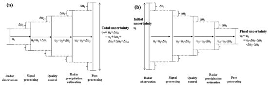
Figure 1.
Definition of uncertainty quantification and propagation in the radar-based precipitation estimation process (a) with increasing uncertainty, (b) with decreasing uncertainty.
2.2. How to Quantify Uncertainty
In this study, the maximum entropy method (MEM), uncertainty Delta method (UDM), and modified-fractional uncertainty method (M-FUM) were used to quantify uncertainty.
2.2.1. Maximum Entropy Method
In discussing information theory, Shannon [26] first introduced the concept of entropy, which has been used widely as a method with which to measure expected values of a given average information content to generate the unpredictability or uncertainty of information. If the probability of occurrence of the given information is large, the amount of information and its uncertainty are small, and vice versa. If the information is a random variable X with probability p, and the average amount of information is defined as I(X), the basic concept of Shannon’s entropy can be described as follows [26]:
where H is entropy of X, x is the value of X, pX(·) is the probability density function of X, and n is the number of x. The principle of maximum entropy (ME), based on Shannon’s entropy theory [26], was first expounded by [27]. It represents the current state of a given information content using the most suitable probability distribution with the largest entropy. When a certain set of information content is given, based on the information content, ME theory can provide the probability density function that maximizes the entropy. ME has the moment constraint () and generalization constraint () [28]. The key concepts of ME and entropy H(x) are as follows:
where fn(·) is the moment constraint and n is the number of samples. If the maximum value b and the minimum value a are given, the distribution maximizing the entropy is a uniform distribution (f(x) = 1/(b − a)) subject to the normalization constraint and the occurrence probabilities of all events are the same on the interval (a, b) [29]. This means the probability of each value of precipitation estimate is equally distributed.
The basic concept of uncertainty propagation in the radar-based precipitation estimation process can be described easily when the above ME is utilized as follows.
First: Radar-based precipitation estimates for all combinations of methods are generated, for example: four methods in the quality control stage, three methods in the precipitation estimation stage, and three methods in the post-processing; all combinations = 24 precipitation estimates.
Second: For a certain method k among all K methods of a certain stage l that is to be demonstrated, the maximum and minimum values of radar-based precipitation estimates where method k is involved, and the corresponding ME Hk,l are calculated, for example: for QC1 method of the quality control stage, 9 precipitation estimates that passes through QC1 method were estimated. For 9 results, the maximum and minimum values were taken to calculate ME.
Third: This process is iterated for all K methods in a given stage l, for example: this process was repeated for three other methods. Each of the four methods had the ME value.
Fourth: The calculated ME in stage l are combined to quantify the averaged uncertainty for stage l. To combine the ME, we may use either the maximum or average operation, for example: in the quality control stage, four ME values were calculated from four methods. The ME in the quality control stage was calculated by averaging four MEs or selecting the maximum value of four MEs.
2.2.2. Uncertainty Delta Method
The Delta method analyzes the variability of each stage using the second-moment “variance” based on a Taylor series expansion. Assuming that the random variable is X and a specific value of x is a, the Taylor series expansion is as follows (ignoring high-order terms):
where specific value a is the average μX of x and y is assumed to be f(x). Then, application of variance to both sides of Equation (4) produces the following:
Using Equation (5), this study improved the Delta method to UDM for quantifying uncertainty. The basic concept of the UDM in quantitative precipitation estimation based on hydrological and weather radar is shown in Figure 2a.
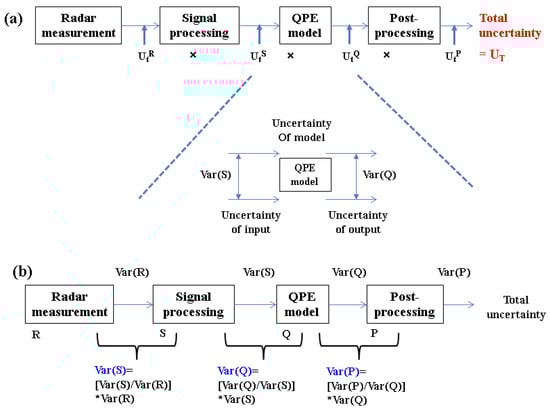
Figure 2.
Basic concept of uncertainty Delta method (UDM): (a) uncertainty quantification and propagation in the precipitation estimation process, (b) quantification in each stage. QPE: quantitative precipitation estimation.
In Figure 2a, the final uncertainty (or total uncertainty) UT can be calculated as variances that occur in the expansion process of Equation (5), which can be expressed as follows:
where R, S, Q, and P represent each stage in the radar-based precipitation estimation process and l(·), h(·), and g(·) are the probability functions of the expectations of the variables at each stage. Then, the uncertainty at each stage can be expressed as by transforming Equation (5). The same expression can be applied to the other stages, which can be summarized as follows:
Equation (7) can be expressed as (total uncertainty) = (uncertainty of post-processing) × (uncertainty of QPE (quantitative precipitation estimation) model) × (uncertainty of signal processing) × (uncertainty of radar measurement). Using this equation, the total uncertainty can be quantified using the variances of each stage. The uncertainty at each stage can be quantified using the variances through Equations (6) and (7), and its process is shown in Figure 2b. By taking the logarithm of both sides of Equation (7), the uncertainty can be quantified. Therefore, the UDM can evaluate the uncertainty at each stage and the total uncertainty.
In comparison with the MEM, which quantifies uncertainty by applying the maximum and minimum values from all radar-based precipitation estimates to Equation (3), the UDM quantifies uncertainty by applying the variances from all precipitation estimates to Equation (7). These two methods are similar in that they use the statistical properties of the range of spread of all precipitation estimates.
2.2.3. Modified-Fractional Uncertainty Method
The uncertainty quantification method proposed by [30] is referred to as the fractional uncertainty method (FUM) in this study. The temporal variability of fractional uncertainty can be represented by the prediction uncertainty divided by the expected mean change () over time for future prediction. This study defined the three sources for uncertainty in radar data as follows: (1) internal variability represents the difference between the simulation result of each method and the average simulation result of all methods. This study used radar-based precipitation estimates and observed values; hence, internal variability is newly conceptualized as the difference between the radar-based precipitation estimates of each method and the station-observed values; (2) scenario uncertainty represents the variance, which means the degree of a spread of various simulation results according to each scenario. This study revised the event uncertainty as the weighted spreading range of precipitation estimates at each event; and (3) method uncertainty represents the average of the variances of all simulation results, and this study used the same concept. With these, the FUM is expressed as the M-FUM, and the basic concepts of each uncertainty are summarized as follows:
Basic concept at each stage
1. Internal uncertainty (V): variance of biases
2. Event uncertainty (E): variance of all precipitation events
3. Model (method) uncertainty (M): average of variances of each method
where i and N represent the specific stages (e.g., quality control, signal processing, and precipitation estimation) and number of stages, respectively; m represents the number of methods; o and x are the observed precipitation and precipitation estimates by simulating method, respectively; W represents the weight of the method, and ε is the difference between the observed precipitation and precipitation estimates by simulating model.
3. Application of Uncertainty Quantification Methods and Results
3.1. Application Outline
3.1.1. Data
Table 1 provides the descriptions of the weather radar precipitation cases used in this study; the application area covers the entire Korean Peninsula. Table 1a lists details of the 11 single-polarization weather radars with maximum scan ranges of 200 km (C-band) and 240 km (S-band), and gate size of 0.25 km, operated by the Korea Meteorological Administration (KMA). It is possible to monitor the entire Korean Peninsula and nearby seas areas using the merged coverage of the 11 radar scan ranges. As planned, all 11 weather radars have recently been replaced by dual-polarization radars, which are currently undergoing test-operations. Table 1b lists details of the 18 precipitation events that occurred in summer (Changma, typhoons, and local precipitation) from June to September 2012–2016.

Table 1.
Summary of the radars and precipitation cases in this study.
3.1.2. Quality Control
This study on precipitation estimation based on weather radars comprised three stages (quality control, precipitation estimation, and post-processing) and quantified the corresponding uncertainties at each stage. In the quality control stage, the fuzzy and open radar product generator (ORPG) algorithms that are applied to single-polarization radar by the KMA Weather Radar Center were implemented [31]. The fuzzy algorithm controls the quality of radar variables by generating membership functions of non-meteorological echoes using statistical analysis with non-ground filtering reflectivity as input variables [31]. In contrast, the ORPG algorithm removes reflectivity above threshold in the application region and corrects reflectivity by applying ground echo filter as input variables.
3.1.3. Quantitative Precipitation Estimation
For the QPE model, the Radar-Automatic Weather Station (AWS) rain rate (RAR) calculation system (hereafter the RAR system), which was developed by the KMA in 2006, was used in this study. The RAR system is operated on site based on the 11 single-polarization radars and 642 AWSs (321 gauges used for calibration and 321 gauges used for validation) located on the Korean Peninsula. In real time, the RAR system generates various merged weather radar precipitation fields for the Korean Peninsula through the following steps: (1) producing the radar reflectivity field of each single radar; (2) calculating AWS precipitation; (3) deriving the Z-R relationship using the window probability matching method (WPMM) [32] or Marshall–Palmer (M–P) relation [33]; (4) estimating precipitation for each single radar; and (5) merging the radar precipitation field for the entire region.
The RAR system implements WPMM [32] using reflectivity and AWS precipitation from the previous hour to estimate radar-based precipitation amounts at each radar site. It then merges the estimated precipitation fields of the radar sites to produce composite precipitation fields for the Korean Peninsula. Quality-controlled reflectivity, with non-meteorological echoes removed, on three-by-three pixels are averaged around each specific AWS location. The WPMM reproduces the probability density functions of ground precipitations from each specific AWS and averaged radar reflectivity, and then determines parameters of the Z-R relationship using these probability density functions to generate radar-based precipitation estimates. These processes are repeated for the 11 single-polarization radars. Thus, various merged radar-precipitation fields for the entire country can be produced using radar-precipitation estimates from each radar. However, appropriate merging methods including maximum value, average value, minimum value, and distance weighting schemes must be advanced because the scan ranges of the radar sites overlap.
3.1.4. Post-Processing
Post-processing precipitation bias correction methods, i.e., the gauge-to-radar (G/R) ratio method of [34] and the local gauge correction (LGC) method of [35], were performed to correct the bias in radar precipitation estimated by the QPE model. The fundamental concept of the G/R method is that the bias correction (G/R ratio) factor, also known as the mean-field bias, is computed as the ratio of the spatial average (mean) between the estimated radar precipitation and observed precipitation in a corresponding area (or point, pixel). Then, the radar-based precipitation estimate multiplied by the G/R ratio factor was calculated to produce corrected precipitation estimates. In this study, radar precipitation estimates tended to be underestimated and all G/R ratio factors were larger than one. The LGC method, which assigns weights to the bias between precipitations observed by the AWSs and the radar-based precipitation estimates, is a modified version of the inverse distance weighting method. The LGC method can correct local bias cases that affect precipitation estimates by modifying the radar precipitation estimates in each pixel. However, the time required to compute the bias in each pixel varies according to the radius of the radar measurement scan.
3.2. Results of Quantitative Radar-Based Precipitation Estimation
As described in Section 3.1, eight ensemble radar-based precipitation estimates were calculated using two quality control algorithms, two precipitation estimation methods, and two post-processing precipitation bias correction methods for the entire Korean peninsula. Following the quality control methods (ORPG and fuzzy algorithms) and the post-processing precipitation bias correction methods (G/R ratio and LGC methods), the accuracy of the radar-based precipitation estimates was compared with the observed precipitation reported by the AWSs (see Table 2). It can be seen from Table 2a that the values of root mean square error (RMSE) and correlation coefficient (CC) relating to the ORPG method were 8.56 mm/h and 0.79, respectively, while those relating to the fuzzy method were 8.32 mm/h and 0.81, respectively. Thus, the accuracy of radar-based precipitation estimates produced using the fuzzy algorithm was superior to that produced using the ORPG method. Table 2b shows the results of the precipitation estimates obtained by applying the G/R ratio and LGC methods to all 18 precipitation events (18 precipitation events × 2 quality control methods). The RMSE and CC values of the G/R ratio method were 7.29 mm/h and 0.93, respectively, while those of the LGC method were 6.06 mm/h and 0.94, respectively. Thus, the accuracy of radar-based precipitation estimates produced using the LGC method, which corrected the bias of the precipitation estimates at each radar pixel, was superior to that produced using the G/R ratio method. Figure 3 shows Q-Q (quantile-quantile) plots of the RMSEs of the radar-based precipitation estimates in each quality control algorithm and bias correction method for the 18 precipitation cases. It can be seen that the RMSEs of the fuzzy algorithm and the LGC method were superior for each precipitation case.
Table 2.
Comparison of the accuracy of radar-based precipitation estimates in each quality control algorithm and bias correction method.
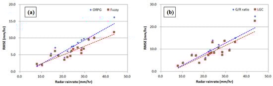
Figure 3.
Q-Q (quantile-quantile) plots of RMSEs of radar-based precipitation estimates in each (a) quality control algorithm and (b) bias correction method.
The results of applying the quality control (fuzzy and ORPG algorithms) and post-processing methods (G/R ratio and LGC methods) are shown in Figure 4. Illustrated in Figure 4a–c are the AWS-observed precipitation and radar-based precipitation estimates produced by applying the fuzzy and ORPG algorithms for case 11, which was an intense precipitation event that occurred in the Incheon and west sea regions at 10:20 local standard time (LST) on 28 August 2012. Although the three panels have slightly different color intensity of the index, this is considered in the comparison of the results.
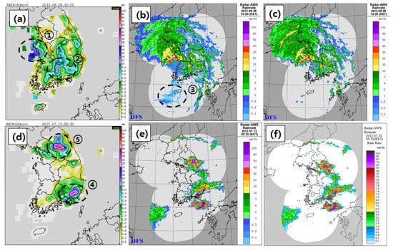
Figure 4.
Comparison of precipitation estimates: between automatic weather stations (AWS) and quality control methods (a) Observation from AWSs, (b) fuzzy, (c) ORPG at 1020 LST on 28 August in 2012; between AWS and bias correction methods (d) AWS, (e) G/R ratio, (f) LGC at 0530 LST on 13 July in 2012.
In Figure 4a, the precipitation intensity in regions ① and ② was 16–20 and 8–12 mm/h, respectively. Precipitation estimates in the same precipitation zones are shown in Figure 4b,c. In region ①, Figure 4c shows very intense precipitation estimates (>40 mm/h in some regions), whereas the precipitation estimates shown in Figure 4b are intense but closer to the observed values. In region ②, the precipitation estimates shown in Figure 4c are more intense than those shown in Figure 4b, which shows precipitation estimates closer to the observed values. However, in region ③ of Figure 4b, the results produced by applying the fuzzy algorithm show wave echoes that have not been removed completely, indicating that the approach requires further improvement.
Illustrated in Figure 4d–f are the AWS-observed precipitation and the radar-based precipitation estimates produced by applying the G/R ratio and LGC algorithms, respectively, for case 6, which was a case of Changma that formed along the east sea coast to the southern sea at 05:30 LST on 13 July 2012. The precipitation observed by the AWSs (Figure 4d) shows very intense precipitation in regions ④ and ⑤; the most intense precipitation was 53.5 mm/h in region ⑤. Precipitation estimates produced by applying the G/R ratio method (Figure 4e) were underestimated considerably throughout the entire area. In contrast, in Figure 4f, precipitation estimates produced by applying the LGC method were more intense than those produced using the G/R ratio method; especially, in relation to the occurrence of the intense precipitation in regions ④ and ⑤ that was relatively well estimated.
The results presented in Figure 4 show that the application of the fuzzy algorithm during quality control and of the LGC method during post-processing produces results that are more accurate for generating radar-based precipitation estimates.
3.3. Results and Discussion of Uncertainty Quantification
3.3.1. Analysis of Quantified Uncertainty
In this study, the uncertainty quantification methods were applied to generate a radar-based precipitation estimate, and the results of the uncertainty quantification are shown in Table 3 and Figure 5. In Table 3 and Figure 5, the results at each stage were obtained by averaging the data from the 18 precipitation events. During installation, radar hardware is adjusted and internally calibrated. In addition, when a weather radar receives signals, it stores data in its internal hardware, which is referred to as level zero. However, it is difficult to access the level zero data through the hardware process. Thus, this study employed the level one data which are produced by applying threshold variable and speckle filter to level zero data. In brief, because of data limitations in the radar-based precipitation estimation process, the signal processing stage was not considered; therefore, the initial uncertainty was assumed to begin with the quality control stage. In the results of applying the MEM, Table 3a and Figure 5a show that the ME values (MEV) of the ORPG and fuzzy algorithms in quality control were 4.28 and 4.15, respectively, the MEVs of the WPMM and M–P relations in precipitation estimation were 3.90 and 4.53, respectively, and the MEVs of the LGC and G/R ratio methods in post-processing were estimated at 3.77 and 3.81, respectively. From these results, it can be determined that the initial uncertainty was 4.28 (same as the MEVs of quality control) and the final uncertainty was estimated at 3.81 (same as the MEVs of the post-processing). Assuming that the final uncertainty was 100%, the MEVs of the quality control stage and the radar-based precipitation estimation stage were 112% and 119%, respectively, which implies that the uncertainty in the radar-based precipitation estimation increased in comparison with the initial uncertainty of the quality control stage. However, the uncertainty then decreased in the post-processing stage, and the final uncertainty was reduced in comparison with the initial uncertainty. The reason is that, although the MEV of the WPMM was 3.90, the MEV of the M–P relation was 4.53, which shows that the M–P relation was the major contributor to the increasing uncertainty in the precipitation estimation stage. This implies that radar-based precipitation estimates and their corresponding uncertainty are dependent on the applied methodology.
Table 3.
Comparison of uncertainty quantification results for each stage in the radar-based precipitation estimation process using the MEM, UDM, and M-FUM.
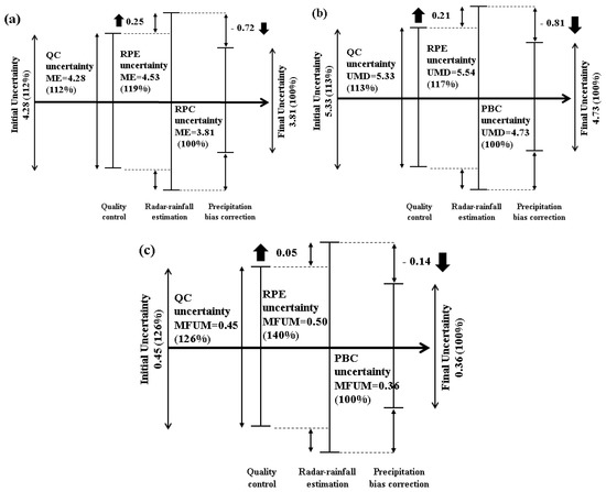
Figure 5.
Uncertainty quantification and propagation in the radar-based precipitation estimation process using (a) the MEM, (b) the UDM, and (c) the M-FUM.
In applying the UDM, the variances of each stage were calculated. Those of the ORPG and fuzzy algorithms in quality control were 206.43 and 121.51 mm2/h2, respectively, those of the WPMM and M–P relations were 145.47 and 254.68 mm2/h2, respectively, and those of the LGC and G/R ratio methods were calculated as 82.45 and 115.58 mm2/h2, respectively. Table 3b and Figure 5b show that the UDM values of the ORPG and fuzzy algorithms in quality control were 5.33 and 4.80, respectively, the UDM values of the WPMM and M–P relations in precipitation estimation were 0.18 and 0.21, respectively and the UDM values of the LGC method and G/R ratio method in post-processing were −0.79 and −0.81, respectively. In considering uncertainty in the UDM, the initial uncertainty was 5.33 (same as the UDM value of quality control) and the final uncertainty was estimated to be 4.75, which was the same as that of the post-processing stage. Assuming that the UDM value of the final uncertainty was 100%, the UDM value of the quality control stage was 113% and that of the radar-based precipitation estimation stage was 117%. This result shows that, similar to the tendency of ME, uncertainty decreased in the post-processing stage in the radar-based precipitation estimation, although it increased in comparison with the initial uncertainty. The final uncertainty also decreased compared to the initial uncertainty. It can be determined that the M–P relation was the major contributor to the increasing uncertainty in the precipitation estimation stage, because the UDM value of the M–P relation was larger than that of the WPMM.
Table 3c and Figure 5c show that the M-FUM values of the ORPG and fuzzy algorithms in quality control were 0.45 and 0.39, respectively, the M-FUM values of the WPMM and M–P relations in precipitation estimation were estimated at 0.44 and 0.50, respectively, and the M-FUM values of the LGC and G/R ratio methods in the post-processing were 0.33 and 0.36, respectively. Although the final uncertainty (0.36) was smaller than the initial uncertainty (=0.45), the uncertainty in the middle stage of the entire process increased in comparison with the initial uncertainty. Assuming that the final uncertainty was 100%, as in the previous methods, the uncertainties of the quality control stage and the radar-based precipitation estimation stage were 126% and 140%, respectively. Hence, although the uncertainty of the subsequent stage increased in comparison with the initial uncertainty, the uncertainty then decreased in the post-processing stage. This change in uncertainty was identical to that of the MEM and UDM.
3.3.2. Discussion of the Uncertainty Quantification
As mentioned above, it was confirmed that the accuracy and uncertainty of radar-based precipitation estimates could be changed depending on the method applied at each stage. In this section, the results provided in the previous section are reanalyzed to determine the superior method for each stage. The fuzzy algorithm in the quality control stage, WPMM in the precipitation estimation stage, and the LGC method in the post-processing stage were selected, and the results of applying these three methods are shown in Figure 6.
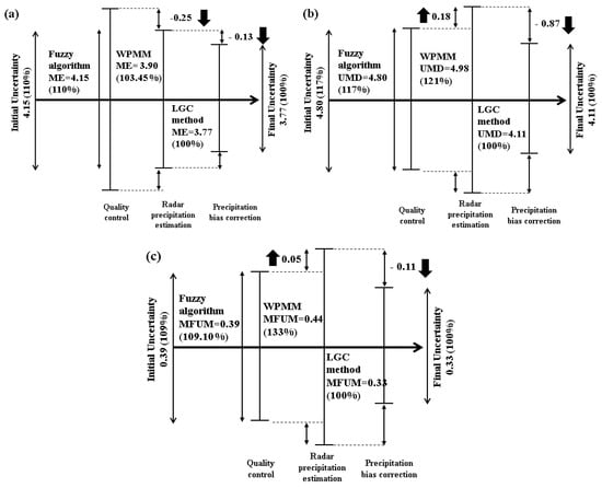
Figure 6.
Uncertainty quantification and propagation in the radar-based precipitation estimation process in case of selected superior methods for each stage using (a) the MEM, (b) the UDM, and (c) the M-FUM.
For the MEM in each stage, the uncertainty gradually decreased, i.e., to 4.15, 3.90, and 3.77 in association with the fuzzy algorithm, WPMM, and LGC method, respectively. Assuming that the final uncertainty in the MEM was 100%, the uncertainty of the fuzzy algorithm was 110%, and that of the WPMM was 103%. However, the uncertainty of the LGC method was 100%, i.e., the same as the final uncertainty. The tendency of uncertainty propagation showed that the major contributor was the quality of the radar measurements, and that the uncertainty was reduced by applying the superior method at each subsequent stage. In contrast, for the UDM and M-FUM, even if the best method was applied at each stage, the uncertainty was propagated in the same way as the quantitative uncertainty when applying the UDM and M-FUM, mainly because all methods in the precipitation estimation stage were major contributors to increasing the uncertainty. This indicates that there might be stages that could increase the uncertainty even if a method that performs well at each stage is selected. In summary, in the entire radar-based precipitation estimation process, selecting a method with superior accuracy in each stage will result in the lowest uncertainty.
4. Summary and Conclusions
In quantitative precipitation estimation based on weather radars, uncertainty propagates at each stage of quality control, precipitation estimation, and post-processing precipitation bias correction. However, existing methods have only improved the understanding and accuracy of the uncertainty at specific stages, and they have not clarified the proportion of uncertainty at each stage related to the total uncertainty. Thus, such methods have been unable to reveal the increase (or decrease) in uncertainty at each stage. Accordingly, this study proposed novel application of three methods for the quantification of uncertainty (i.e., the MEM, UDM, and M-FUM). The MEM was selected to assess uncertainty quantitatively using the ME, which has been used widely for uncertainty quantification. The UDM was developed to analyze the uncertainty at each stage using the ratio of variances of each method based on a Taylor series expansion. Then, the M-FUM modified three uncertainty sources of the FUM to estimate uncertainty in the radar-based precipitation estimation process.
To test the applicability of the three methods, this study implemented a radar-based precipitation estimation process for the Korean Peninsula, which consisted of two quality control algorithms, two precipitation estimation methods, and two post-processing precipitation bias correction methods in relation to 18 precipitation events that occurred during 2012 to 2016. It was shown that the radar-based precipitation estimates and their corresponding uncertainty could vary depending on the precipitation estimation method applied. In addition, it was revealed that the uncertainty propagation of the MEM, together with the fuzzy algorithm in the quality control stage, WPMM in the precipitation estimation stage, and the LGC method in the post-processing stage could reduce the uncertainty. However, the UDM and M-FUM were responsible for the uncertainty propagation in the same manner as the quantitative uncertainty. Consequently, selecting a method with superior accuracy at each stage will result in the lowest uncertainty.
Through the novel use of the three uncertainty quantification methods proposed herein, the following advancements could be expected for radar-based precipitation estimation. First, uncertainty could be quantified for the entire process and for each stage. Second, the ratios of uncertainty at each stage to the total uncertainty could be identified. Finally, the uncertainty propagation process could be demonstrated at each stage of the process. With these benefits, the major contributor to uncertainty in radar-based precipitation estimation will be better understood and its impact reduced more effectively.
Author Contributions
Conceptualization, J.-K.L.; methodology, J.-K.L.; investigation, J.-K.L.; writing—original draft preparation, J.-K.L.; writing—review and editing, C.G.S.; supervision, C.G.S.; project administration, C.G.S.; funding acquisition, C.G.S. All authors have read and agreed to the published version of the manuscript.
Funding
This research received no external funding.
Acknowledgments
This work is supported by the Korea Agency for Infrastructure Technology Advancement (KAIA) grant funded by the Ministry of Land, Infrastructure and Transport (Grant 20DPIW-C153746-02).
Conflicts of Interest
The authors declare no conflict of interest.
References
- Huff, F.A. Sampling errors in measurement of mean precipitation. J. Appl. Meteorol. 1970, 9, 35–44. [Google Scholar] [CrossRef]
- Woodley, W.; Olsen, A.; Herndon, A.; Wiggert, V. Comparison of gage and radar methods of convective rain measurement. J. Appl. Meteorol. 1975, 14, 909–928. [Google Scholar] [CrossRef][Green Version]
- Wilson, J.W.; Brandes, E.A. Radar measurement of rainfall: A Summary. Bull. Am. Meteorol. Soc. 1979, 60, 1048–1058. [Google Scholar] [CrossRef]
- Austin, P.M. Relation between measured radar reflectivity and surface rainfall. Mon. Weather Rev. 1987, 115, 1053–1070. [Google Scholar] [CrossRef]
- Campos, E.; Zawadzki, I. Instrumental uncertainties in Z–R relations. J. Appl. Meteorol. 2000, 39, 1088–1102. [Google Scholar] [CrossRef]
- Krajewski, W.F.; Smith, J. Radar hydrology: Rainfall estimation. Adv. Water Resour. 2002, 25, 1387–1394. [Google Scholar] [CrossRef]
- Shakti, P.C.; Maki, M. Application of a modified digital elevation model method to correct radar reflectivity of X-band dual-polarization radars in mountainous regions. Hydrol. Res. Lett. 2014, 8, 77–83. [Google Scholar] [CrossRef]
- Park, S.G.; Bringi, V.N.; Chandrasekar, V.; Maki, M.; Iwanami, K. Correction of radar reflectivity and differential reflectivity for rain attenuation at X band. Part I: Theoretical and empirical basis. J. Atmos. Ocean. Technol. 2005, 22, 1621–1632. [Google Scholar] [CrossRef]
- Park, S.G.; Maki, M.; Iwanami, K.; Bringi, V.N.; Chandrasekar, V. Correction of radar reflectivity and differential reflectivity for rain attenuation at X band. Part II: Evaluation and application. J. Atmos. Ocean. Technol. 2005, 22, 1633–1655. [Google Scholar] [CrossRef]
- Villarini, G.; Krajewski, W.F. Empirically-based modeling of spatial sampling uncertainties associated with rainfall measurements by rain gauges. Adv. Water Resour. 2008, 31, 1015–1023. [Google Scholar] [CrossRef]
- Sebastianelli, S.; Fabio, R.; Napolitano, F.; Baldini, L. On precipitation measurements collected by a weather radar and a rain gauge network. Nat. Hazard Earth Syst. 2013, 13, 605–623. [Google Scholar] [CrossRef]
- Jordan, P.; Seed, A.; Austin, G. Sampling errors in radar estimates of rainfall. J. Geophys. Res. 2000, 105, 2247–2257. [Google Scholar] [CrossRef]
- Villarini, G.; Krajewski, W.F. Sensitivity studies of the models of radar-rainfall uncertainties. J. Appl. Meteorol. Clim. 2010, 49, 288–309. [Google Scholar] [CrossRef]
- Moulin, L.; Gaume, E.; Obled, C. Uncertainties in mean areal precipitation: Assessment and impact on streamflow simulations. Hydrol. Earth Syst. Sci. 2009, 13, 99–114. [Google Scholar] [CrossRef]
- Kim, D.-S.; Kang, M.-Y.; Lee, D.-I.; Kim, J.-H.; Choi, B.-C.; Kim, K.E. Reflectivity Z and differential reflectivity ZDR correction for polarimetric radar rainfall measurement. In Proceedings of the Spring Meeting of Korean Meteorological Society, Goyang-si Kintex, Korea, 12 October 2006; pp. 130–131. [Google Scholar]
- Germann, U.; Galli, G.; Boscacci, M.; Bolliger, M. Radar precipitation measurement in a mountainous region. Q. J. R. Meteor. Soc. 2006, 132, 1669–1692. [Google Scholar] [CrossRef]
- Ciach, G.J.; Krajewski, W.F. On the estimation of radar rainfall error variance. Adv. Water Resour. 1999, 22, 585–595. [Google Scholar] [CrossRef]
- Ciach, G.J.; Krajewski, W.F.; Villarini, G. Product-error-driven uncertainty model for probabilistic quantitative precipitation estimation with NEXRAD data. J. Hydrometeorol. 2007, 8, 1325–1347. [Google Scholar] [CrossRef]
- Zhang, Y.; Adams, T.; Bonta, J.V. Subpixelscale rainfall variability and the effects on the separation of radar and gauge rainfall errors. J. Hydrometeorol. 2007, 8, 1348–1363. [Google Scholar] [CrossRef]
- Oh, H.-M.; Ha, K.-J.; Kim, K.-E.; Bae, D.-H. Precipitation rate combined with the use of optimal weighting of radar and rain gauge data. Atmos. Korean Meteorol. Soc. 2003, 13, 316–317. [Google Scholar]
- Yoo, C.; Kim, J.; Yoon, J.; Park, C.; Park, C.; Jun, C. Use of the Kalman filter for the correction of mean-field bias of radar rainfall. In Proceedings of the 5th Korea-Japan-China Joint Conference on Meteorology, Busan, Korea, 24–26 October 2011. [Google Scholar]
- Krajewski, W.F.; Villarini, G.; Smith, J.A. Radar-rainfall uncertainties. Bull. Am. Meteorol. Soc. 2010, 91, 87–94. [Google Scholar] [CrossRef]
- McMillan, H.; Jackson, B.; Clark, M.; Kavetski, D.; Woods, R. Rainfall uncertainty in hydrological modeling: An evaluation of multiplicative error models. J. Hydrol. 2011, 400, 83–94. [Google Scholar] [CrossRef]
- Jones, R.N. Managing uncertainty in climate change projections—Issues for impact assessment: An editorial comment. Clim. Change 2000, 45, 403–419. [Google Scholar] [CrossRef]
- IPCC. Climate Change 2001: Impacts, Adaptations, and Vulnerability; Contribution of Working Group II to the Third Assessment Report of the Intergovernmental Panel on Climate Change; Cambridge University Press: Cambridge, UK; New York, NY, USA, 2001. [Google Scholar] [CrossRef]
- Shannon, C.E. A Mathematical Theory of Communication. Bell Syst. Tech. J. 1948, 27, 379–423. [Google Scholar] [CrossRef]
- Jaynes, E.T. Information theory and statistical mechanics. Phys. Rev. 1957, 106, 620–630. [Google Scholar] [CrossRef]
- Gay, C.; Estrada, F. Objective probabilities about future climate are a matter of opinion. Clim. Chang. 2010, 99, 27–46. [Google Scholar] [CrossRef]
- Kottegoda, N.T.; Rosso, R. Statistics, Probability, and Reliability for Civil and Environmental Engineers; McGraw-Hill: New York, NY, USA, 1997; pp. 61–64. [Google Scholar]
- Hawkins, E.D.; Sutton, R. The potential to narrow uncertainty in regional climate predictions. Bull. Am. Meteorol. Soc. 2009, 90, 1095–1107. [Google Scholar] [CrossRef]
- Weather Radar Center. Weather Radar Data Analysis Guidance; Weather Radar Center Technical Note; Weather Radar Center: Seoul, Korea, 2013.
- Rosenfeld, D.; Wolff, D.B.; Amitai, E. The window probability matching method for rainfall measurements with radar. J. Appl. Meteorol. 1994, 33, 682–693. [Google Scholar] [CrossRef][Green Version]
- Marshall, J.S.; Langille, R.C.; Palmer, W.M.K. Measurement of rainfall by radar. J. Meteorol. 1947, 4, 186–192. [Google Scholar] [CrossRef]
- Morin, E.; Maddox, R.A.; Goodrich, S.; Sorooshin, S. Radar Z-R Relationship for summer monsoon storm in Arizona. Weather Forecast 2005, 20, 672–679. [Google Scholar] [CrossRef]
- Zhang, J.; Howard, K.; Langston, C.; Vasiloff, S.; Kaney, B.; Arthur, A.; Van Cooten, S.; Kelleher, K.; Kitzmiller, D.; Ding, F. National mosaic and multi-sensor QPE (NMW) system. Bull. Am. Meteorol. Soc. 2011, 92, 1321–1338. [Google Scholar] [CrossRef]


Publisher’s Note: MDPI stays neutral with regard to jurisdictional claims in published maps and institutional affiliations. |
© 2020 by the authors. Licensee MDPI, Basel, Switzerland. This article is an open access article distributed under the terms and conditions of the Creative Commons Attribution (CC BY) license (http://creativecommons.org/licenses/by/4.0/).