Online Reinforcement Learning-Based Control of an Active Suspension System Using the Actor Critic Approach

Abstract

In this paper, a controller learns to adaptively control an active suspension system using reinforcement learning without prior knowledge of the environment. The Temporal Difference (TD) advantage actor critic algorithm is used with the appropriate reward function. The actor produces the actions, and the critic criticizes the actions taken based on the new state of the system. During the training process, a simple and uniform road profile is used while maintaining constant system parameters. The controller is tested using two road profiles: the first one is similar to the one used during the training, while the other one is bumpy with an extended range. The performance of the controller is compared with the Linear Quadratic Regulator (LQR) and optimum Proportional-Integral-Derivative (PID), and the adaptiveness is tested by estimating some of the system’s parameters using the Recursive Least Squares method (RLS). The results show that the controller outperforms the LQR in terms of the lower overshoot and the PID in terms of reducing the acceleration.

1. Introduction

Ride quality and passenger comfort are some of the major concerns of any vehicle designer and have been well investigated and researched over the past few decades. The vehicle suspension system plays an important role in vehicle safety, handling, and comfort. It keeps the tires in contact with the road, provides good handling and stable steering, and minimizes the vibrations and oscillations due to road irregularities, which ensure the comfort of the passengers. In general, the suspension is divided into three types: passive, semi-active, and active suspension systems. Most of today’s vehicles use the passive system, which consists of a spring and a damper that are fixed at the design stage, which provide an acceptable performance for a limited frequency range. Changing the suspension properties like the damping coefficient allows for good performance, but in a different frequency range. That is why sport cars have better handling than standard cars, whereas the latter have better riding quality. In a semi-active suspension system, energy is not added to the system; however, the system varies the viscous damping co-efficient of the shock absorber. Therefore, the need for a system that attains the objectives for the entire working frequency range justifies the momentum for active suspension research.

In the active suspension system, an actuator is added to the spring and damper, which adds energy to the system by exerting an adaptive counter force, resulting in an improved dynamics behavior. Several controllers were implemented in the active suspension system problem, and the discrete indirect pole assignment with a fuzzy logic gain scheduler was developed by [1]. A non-linear model of the active suspension was investigated by [2] using a sliding mode controller that utilizes the sky-hook damper system without the need for road profile input. There have been more recent attempts to improve the system such as the study conducted by [3], which used two loop PID applied to the half model in the non-linear form. Compared to the passive system with the same parameters, they showed excellent improvement. However, the controller could not completely reject the disturbance. Another example of the utilization of the PID controller in the half model was that developed by [4]. They studied three scenarios and tried three tuning methods where the iterative learning algorithm performed better than the other two methods. Reference [5] showed that fuzzy logic performed significantly better than the PID in the quarter model based on two types of road conditions. Another comparison based on the quarter model, but between a robust PI and Linear Quadratic Regulator (LQR) controller, was conducted by [6], where they showed that the LQR outperformed the PI controller in the presence of parameter uncertainty. Another optimal controller is $H_{\infty }$, which was examined by [7] and showed a 93% reduction in the car’s acceleration, wheel travel, and suspension travel.

Recently, machine learning has been widely investigated in control problems and applied to vehicle suspension. In many cases, neural networks are used in combination with traditional controllers including the sliding mode controller [8], PID [9], and LQR [10] to enhance the controller performance and other tasks like determining the road roughness [11], but they have rarely been used as the controller itself. A good example that motivates the use of machine learning methods as the controller is [12], where a neural network was trained by the optimal PID and surpassed it under parameter uncertainties. Another machine learning method that has recently gained momentum and shown great success in a broad range of applications including games and economics, but rarely applied to control problems, is reinforcement learning.

Despite the rare application of reinforcement learning in the active suspension problem, one of the earliest attempts to the best of our knowledge was conducted by [13,14,15]. Although there is a significant difference between their learning algorithms and the currently used algorithms, the core idea of learning by interactions and experience is the same. The three attempts shared the same idea of maximizing a cost function and learning to select the controller parameters to achieve the best performance. The learning algorithm implemented by [13] was able to achieve near optimal results compared with the Linear Quadratic Gaussian (LQG) under idealized conditions. Reference [15] had the same approach, but they introduced a new learning scheme, which allowed the controller after learning to work in certain conditions where the traditional LQG controller resulted in an unstable system. They also tested the learning method in a real vehicle, but with a semi-active suspension system installed, and they showed promising experimental results. A more recent successful attempt was the study done by [16] where they applied a stochastic real-valued reinforcement learning control to a non-linear quarter model. A similar approach to the one considered in this research was conducted by [17]; the actor critic networks were trained by the policy gradient method, and the controller was tested to some extent with the same road profile considered in this study. They compared their work with the passive suspension system and showed 62% improvement.

In this paper, an online deep reinforcement learning controller is developed using the TD advantage actor critic algorithm. The controller is applied to a quarter model active suspension system to investigate the performance of this learning-based algorithm against the Linear Quadratic Regulator (LQR) and the optimum Proportional-Integral-Derivative (PID). In order to handle possible system uncertainties, the algorithm is integrated with a Recursive Least Squares method (RLS) for online estimation of system damping coefficients.

2. Methods

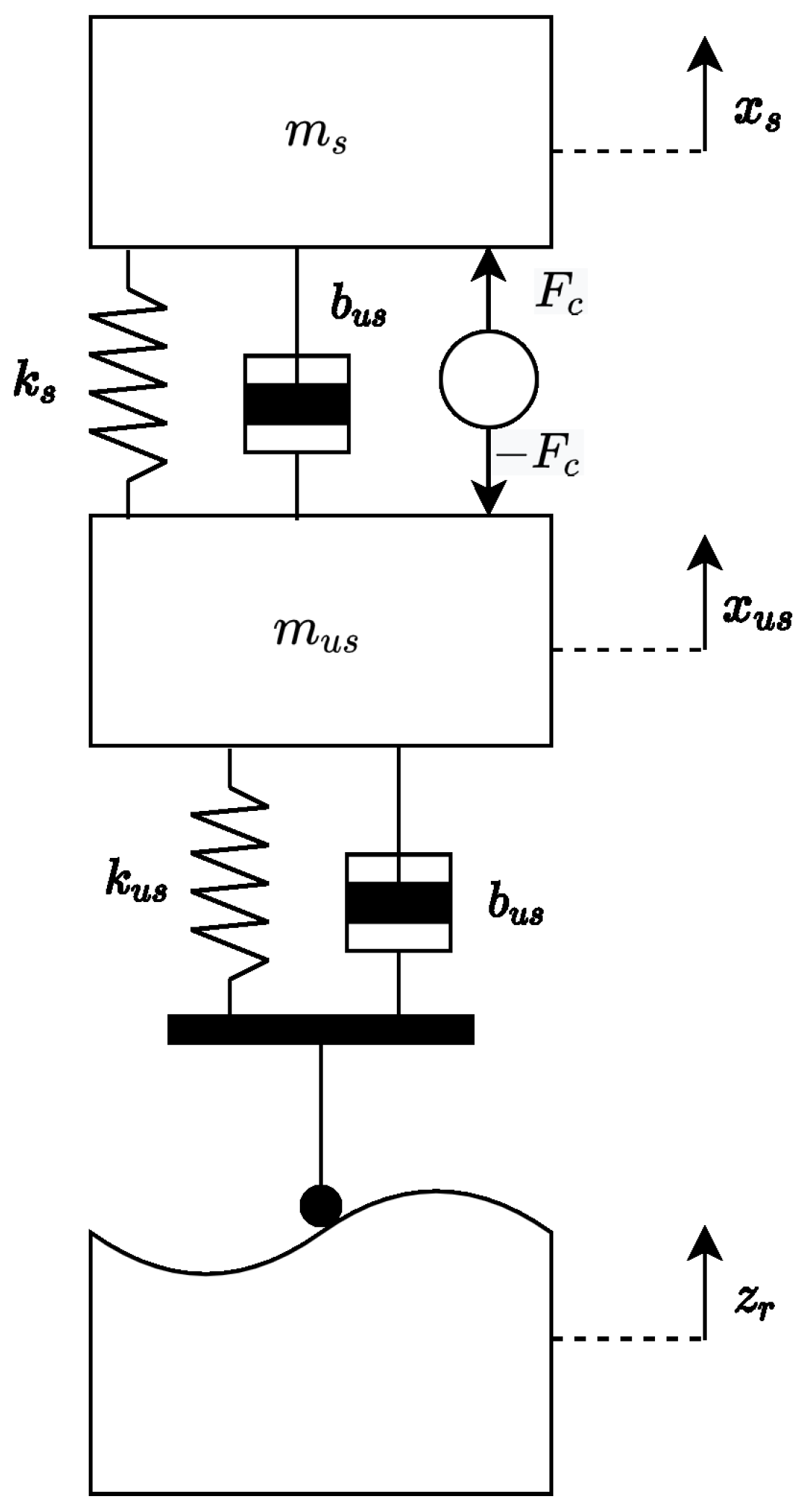
2.1. Modeling of the Active Suspension System

The active suspension model considered in this paper is the linear quarter model shown in Figure 1. It consists of two masses supported by two dampers and two springs. The first one is the sprung mass $m_s$, which represents the vehicle body and is supported by the suspension, which is modeled by the damper $b_s$ and $k_s$. The wheel mass and the tire contact with the road are represented by the unsprung mass $m_{us}$, the damper $b_{us}$, and the stiffness $k_{us}$, respectively. The nominal values considered in this study are shown in

Table 1. Nominal model parameters.

Parameter	Value
Sprung mass $m_s$	2.45 kg
Damping of the car body damper $b_s$	7.5 s/m
Stiffness of the car body $k_s$	900 N/m
Unsprung mass $m_{us}$	1 kg
Damping of tire $b_{us}$	5 s/m
Stiffness of the tire $k_{us}$	2500 N/m

, and the mathematical model of the active suspension is represented by the following state space:

$$\dot{\mathit{x}}=\mathit{Ax}+\mathit{Bu}+\mathit{d}$$

(1)

$$\mathit{y}=\mathit{Cx}+\mathit{D}u$$

(2)

$$\mathit{A}=\left[\begin{array}{cccc}0& 1& 0& 0\\ -\frac{k_s}{m_s}& -\frac{b_s}{m_s}& \frac{k_s}{m_s}& \frac{b_s}{m_s}\\ 0& 0& 0& 1\\ \frac{k_s}{m_{us}}& \frac{b_s}{m_{us}}& -\frac{k_s+k_{us}}{m_{us}}& -\frac{b_s+b_{us}}{m_{us}}\end{array}\right]\mathit{B}=\left[\begin{array}{c}0\\ \frac{1}{m_s}\\ 0\\ -\frac{1}{m_{us}}\end{array}\right]\mathit{d}=\left[\begin{array}{c}0\\ 0\\ 0\\ \frac{b_{us}}{m_{us}}{\dot{z}}_r+\frac{k_{us}}{m_{us}}{z}_r\end{array}\right]\mathit{x}=\left[\begin{array}{c}{x}_s\\ {\dot{x}}_s\\ x_{us}\\ {\dot{x}}_{us}\end{array}\right]$$

$$\mathit{y}=\left[\begin{array}{c}{x}_s-x_{us}\\ {\ddot{x}}_s\end{array}\right]u=F_c$$

$$\mathit{C}=\left[\begin{array}{cccc}1& 0& -1& 0\\ -\frac{k_s}{m_s}& -\frac{b_s}{m_s}& \frac{k_s}{m_s}& \frac{b_s}{m_s}\end{array}\right]\mathit{D}=\left[\begin{array}{c}0\\ \frac{1}{m_s}\end{array}\right]$$

The states are defined as: the displacement of the sprung mass $x_s$, the vehicle body velocity ${\dot{x}}_s$, the displacement of the unsprung mass $x_{us}$, and the vertical velocity of the wheel ${\dot{x}}_{us}$. Other states can be obtained such as the suspension travel $x_s-x_{us}$ and the wheel relative deflection with respect to the road profile $x_{us}-z_r$. $z_r$ and ${\dot{z}}_r$ represent the changes of the road profile and the rate of its change.

The actuator is positioned between the sprung and unsprung mass and generates a counter force to improve the system performance by reducing the acceleration and the suspension travel. The open loop response of the system can be obtained by setting $F_c=0$, which corresponds to the performance of the passive suspension system. We assume the working of the actuator, also referred to as the action space later, to be between −60 N and 60 N.

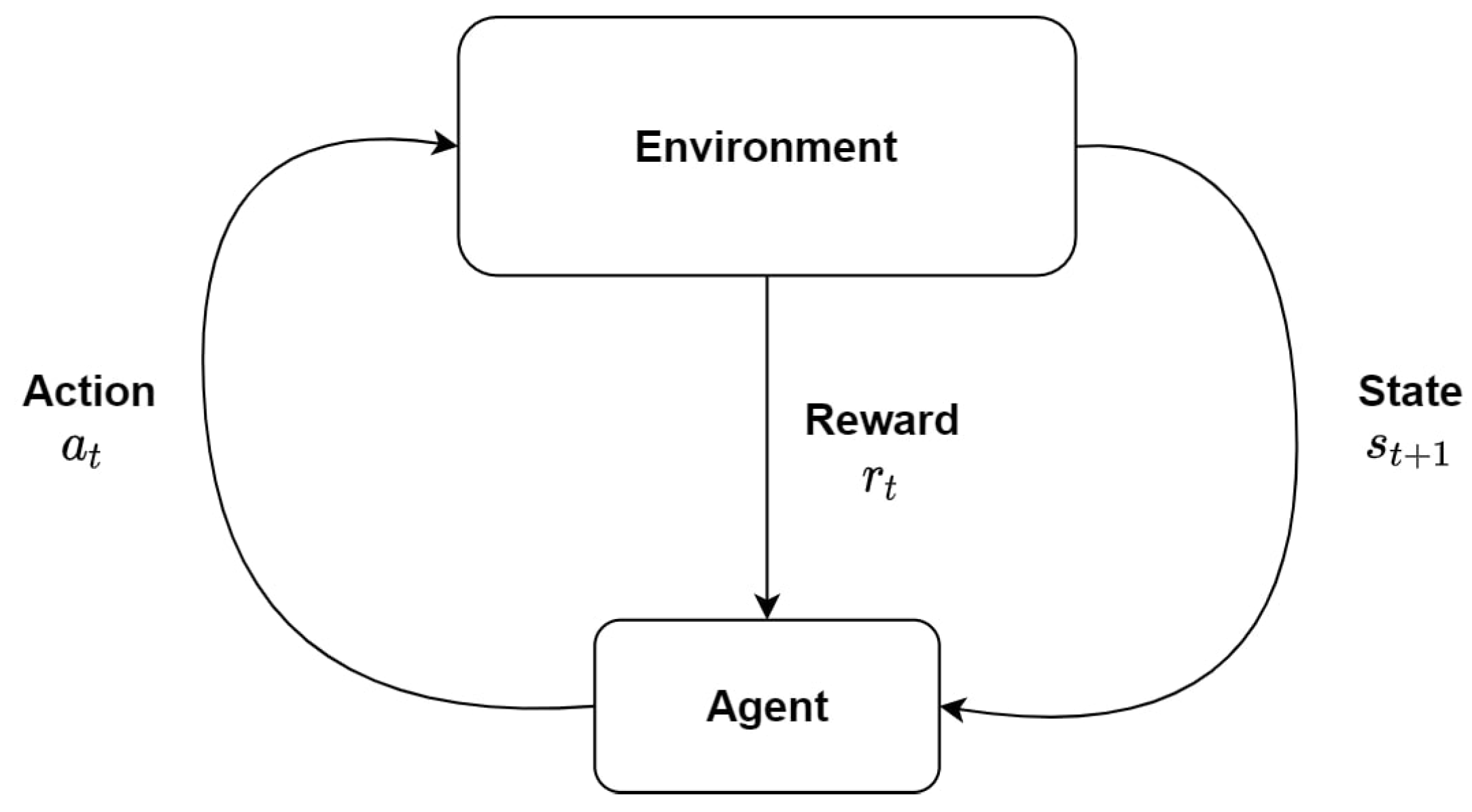
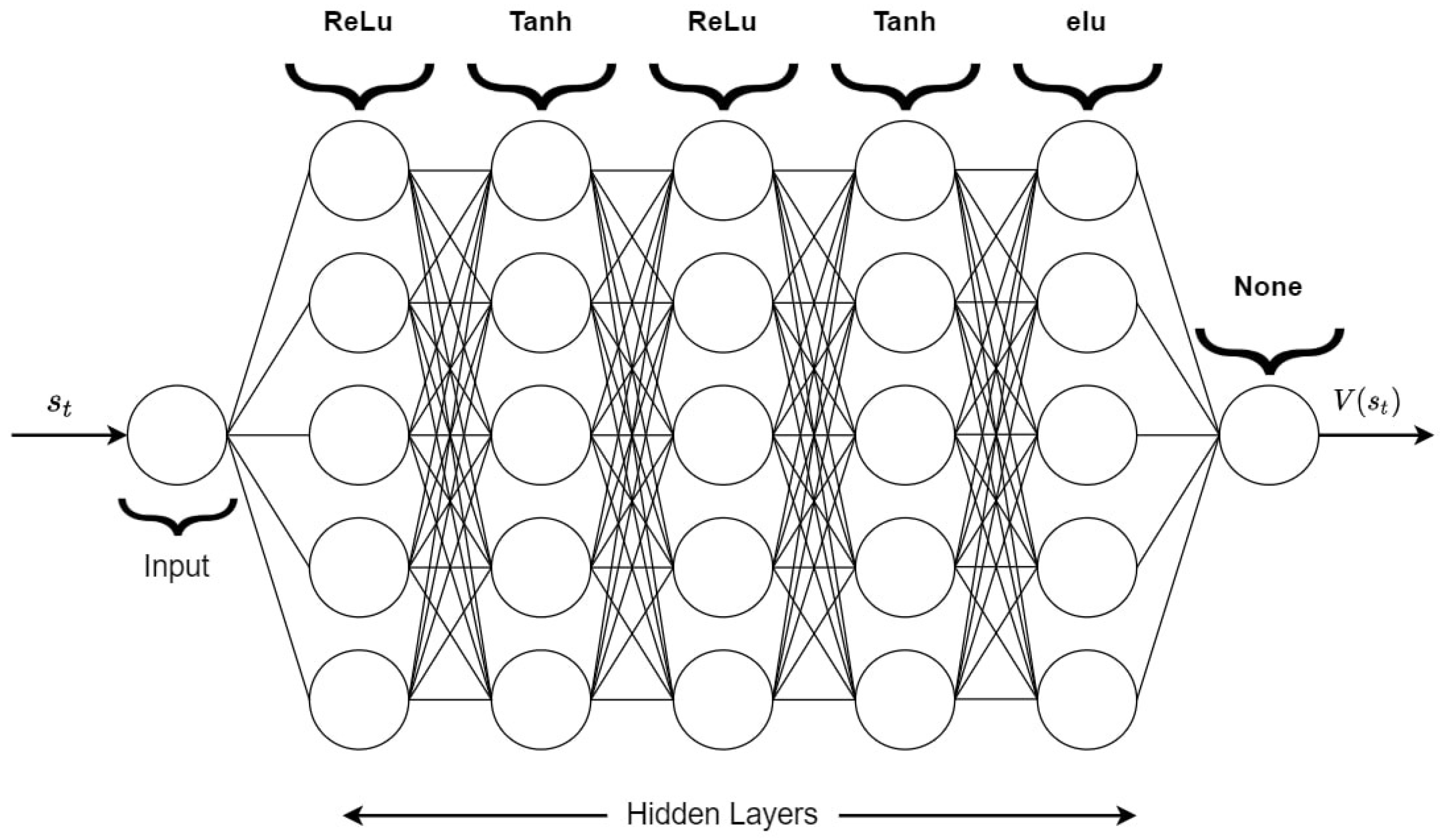
2.2. Reinforcement Learning

Reinforcement learning is one of the three machine learning methods that has witnessed in the past few years a significant leap due to hardware improvements, especially after the publication of the first successful deep learning model that learned to control the policies of seven Atari 2600 games [18]. As shown in Figure 2, reinforcement learning works by the concept of trial and error where an agent at a certain state $s_t$ takes an action $a_t$ to interact with the environment, steps to a new state $s_{t+1}$, and gets a reward that depends on the value of the new state, which therefore reflects the quality of the action taken by the agent. The target is to find a policy ${\pi }^{\theta }$ that maximizes the accumulated reward, subsequently. It can be said that the agent learns by experience. This method has gained much attention due to its ability to solve complex problems that cannot be solved by supervised learning efficiently without the need for huge training datasets and correct answers that are passed to the neural network through backpropagation. It can also overtake traditional controllers that work in a bounded range and has limitations when applied to non-linear models and MIMO systems. In this paper, the agent, the environment, and the action represent the controller, the active suspension model, and the force, respectively.

Deep reinforcement learning utilizes neural networks to generate an action $a_t$ given state $s_t$ and estimates the value of a state $s_{t+1}$, which allows us to extend reinforcement learning to the continuous space and continuous action problems. In this paper, we investigate deep reinforcement learning in control problems by applying the TD advantage actor critic algorithm to the active suspension system.

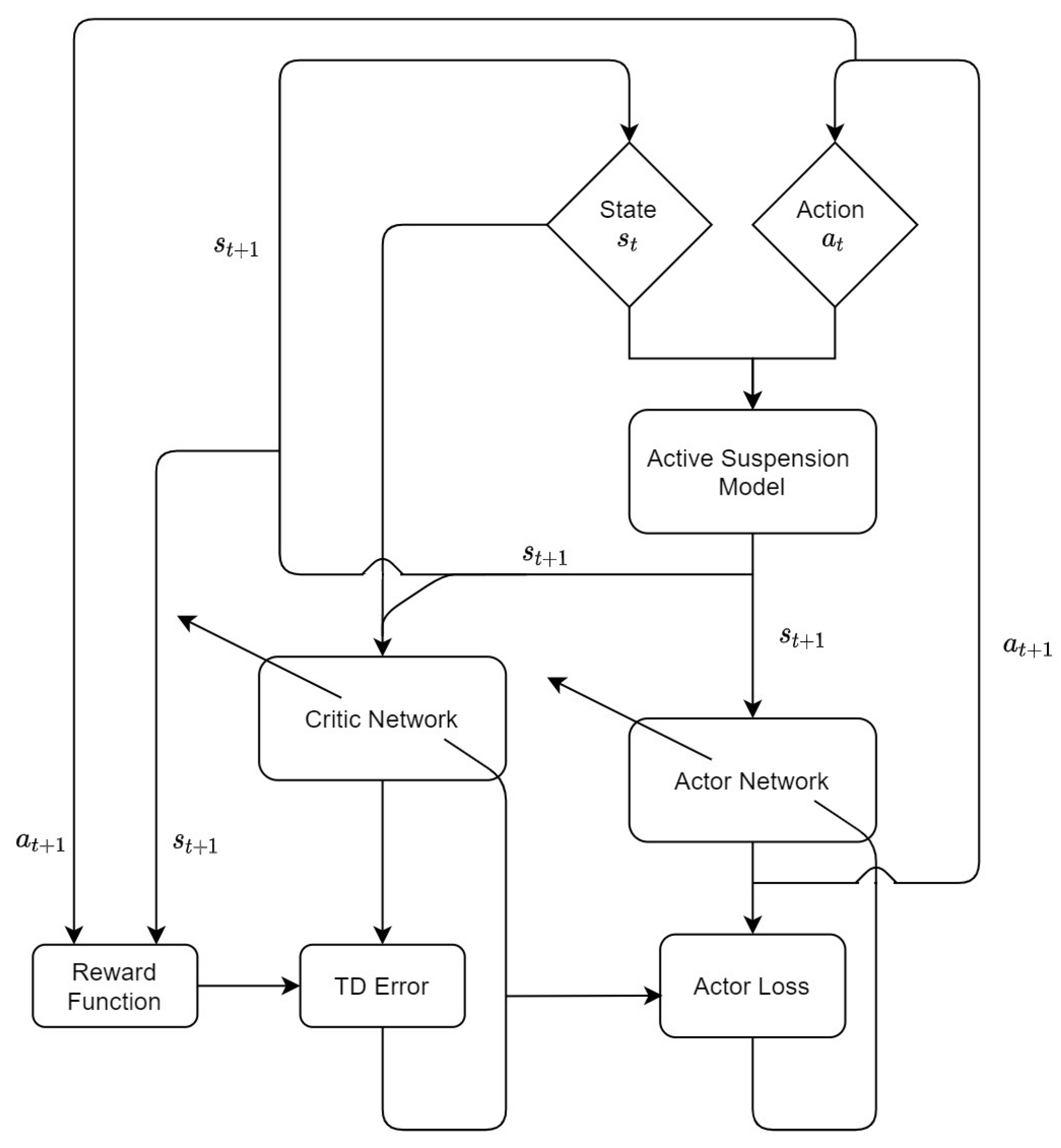
2.2.1. TD Advantage Actor Critic Algorithm

The TD advantage actor critic algorithm is an online model-free algorithm that consists of two neural networks, the actor network ${\pi }^{\theta }\left(s\right)$ and the critic network $V_{\pi }^U\left(s\right)$, where $\theta$ is the actor network parameters (weights and biases) and U is the critic network parameters (weights and biases). The actor network takes the current state $s_t$ as an input and generates an action $a_t$ given the current policy ${\pi }^{\theta }$, and the agent executes the action in the environment, which therefore produces a scalar reward signal $r_t$ and steps to the next state $s_{t+1}$. The critic network takes the current state as an input and produces a value for that state $V_{\pi }^U\left(s\right)$, then the next state is fed to the critic network to produce a value for it $V_{\pi }^U\left(s_{t+1}\right)$ before the parameters are updated. The critic learns a value function, which is then used to update the actor’s weights in the direction of improving the performance at every time step.

In this algorithm, the output of the actor is not the action itself; this is the mean $\mu$ and the standard deviation $\sigma$, which give the probability distribution of choosing action $a_t$ given the state $s_t$. Therefore, the policy is not deterministic; it is a stochastic policy. A step by step implementation is shown in Algorithm 1.

Algorithm 1: TD Advantage Actor Critic.

Initialize the Critic Network $V_{\pi }^U\left(s\right)$ and the Actor Network ${\pi }^{\theta }\left(s\right)$

for episode = 1:M

Start from the initial state $s_{t_o}$

for i = 1:N

Sample action $a_t\sim {\pi }^{\theta }\left(s_t\right|\mu ,\sigma )=N\left(s_t\right|\mu ,\sigma )$

Execute action $a_t$ in the environment and obtain the reward r and step to the next state $s_{t+1}$

Calculate the temporal difference error ${\delta }_t=r+\gamma V_{\pi }^U\left(s_{t+1}\right)-V_{\pi }^U\left(s\right)$

Update the Critic parameters by minimizing ${\delta }_t^2$

Update the Actor parameters by minimizing the Loss = $-log\left(N\left(s_t\right|\mu ,\sigma )\right)·{\delta }_t$

Set $s_t=s_{t+1}$

end

end

2.2.2. Reward Function

The formulation of the reward function plays a crucial role in the learning process. It is used to indicate the quality of the action taken by the agent after it steps to the next state. In supervised learning, the correct answer is known and fed to the neural network through backpropagation which with using an appropriate optimization method, tunes the network parameters to the direction of minimizing the error. However, in reinforcement learning, the agent receives a reward signal from the environment based on the next state which determines the quality of the taken action. Positive rewards encourage the agent to accumulate as much reward as possible whereas negative rewards incentivize the agent to reach the targeted state quickly to avoid accumulating penalties. We tested three different reward functions, the first one takes the following form:

$$r_t=-k\left(\right|x_s-x_{us}\left|\right)$$

(3)

The second one is as follows:

$$r_t=-k\left(\right|\dot{x_s}\left|\right)$$

(4)

The third reward function is:

$$r_t=-k_1{\left({\dot{x}}_s\right)}^2-k_2\left(\right|u\left|\right)$$

(5)

During the learning process, the third reward function performed the best. The neural networks struggled to converge with the first reward function due to low and close numerical values. The second reward function performed better; however, the actor network was not able to eliminate the steady-state error of the sprung mass $x_s$. The reason for this is that the system can reach zero ${\dot{x}}_s$, therefore obtaining the maximum reward in this case without reaching the desired $x_s$. This problem was solved in the third reward function by adding a small penalty on the force, which will encourage the actor to produce zero forces when ${\dot{x}}_s$ is zero.

In the third reward function, the vehicle body velocity is used as the indicator of the quality for the action taken; the value is squared for a gradual feedback and to benefit from the optimization properties of a convex, thus allowing the controller to know that it is improving. The signal is amplified because the range of the suspension travel being studied is within a few centimeters, and the negative sign is applied to have the reward increased as ${\dot{x}}_s$ decreases, which therefore motivates the controller to reach the desired state as fast as possible. $k_1$ and $k_2$ are chosen to be 1000 and 0.1, respectively. $k_1$ is chosen to have a high value to motivate the controller to reach zero velocity, while $k_2$ is chosen to have a much smaller value as higher values impose limitations on the working range of controller force, which therefore will have a negative impact on the response. Other values might improve or worsen the learning process.

2.2.3. Learning and Optimization

The critic network and actor network structures are shown in Figure 3 and Figure 4, respectively, and the implementation of the algorithm is illustrated in Figure 5. Weights are initialized using variance scaling for Tanh and Sigmoid, Xavier for ReLu, and elu, whereas layers with the linear activation function are initialized from a uniform distribution. The mean output layer $\mu$ is initialized with $\mu$ = 0 and $\sigma$ = 0.5. The vehicle body velocity ${\dot{x}}_s$ is utilized to represent the state of the suspension system and used as the input to both networks. The loss functions for both networks are minimized using the adaptive learning rate algorithm ADAM optimizer, which can be found in [19]. The learning rates for the critic network are chosen to be higher than the actor network such that the critic learns faster; thus, it produces accurate values for the states, which then help the actor learn and generate better actions. The learning rates are 0.01 and 0.001, respectively, and after a marked learning and improvement, the learning rates are decreased to 0.001 and 0.0001, respectively. In many cases, the experience ($s_t,a_t,r_t,s_{t+1}$) is stored in a memory with a pre-defined size, and the networks’ parameters are updated by computing the average gradient over sampled transitions at every time step. While this approach solves the problem of correlated states, however, it is not considered in this paper. Computing the gradients at each time step for the single experience was faster and more efficient since the road profile changes every 1.5 s. The value of the discount factor $\gamma$ was chosen to be 0.99, and the activation functions used throughout our study are summarized in

Table 2. List of activation functions.

Type	Function	Derivative
Linear	$f\left(x\right)=x$	1
Tanh	$f\left(x\right)=\frac{2}{(1+e^{-2x})}-1$	$1-f{\left(x\right)}^2$
Sigmoid	$f\left(x\right)=\frac{1}{1+e^{-x}}$	$f\left(x\right)(1-f(x\left)\right)$
ReLu	$f\left(x\right)=xfor\ge 0$ $f\left(x\right)=0for<0$	1 0
elu	$f\left(x\right)=xfor\ge 0$ $f\left(x\right)=\alpha (e^x-1)for<0$	1 $f\left(x\right)+\alpha$
Sofmax	$f\left(x_i\right)$ = $\frac{e^{x_i}}{{\sum }_{j=1}^k{e}^{x_j}}$	$f\left(x_i\right)({\delta }_{ik}-f\left(x_k\right))$ ${\delta }_{ik}=1fori\ne kand0fori=k$

.

Unfortunately, there is no standard method of choosing the number of neurons, the number of hidden layers, the types, and the order of activation functions. Therefore, we built and ran various models of the actor and critic multiple times until satisfactory performance was achieved. The best performing neural networks in this study are summarized in

Table 3. Various actor-critic models.

Number	Actor						Critic						Accumulated Rewards
1	Hidden Layers Number of Neurons: 5				Output Layers		Hidden Layers Number of Neurons: 18					Output Layer	−16,034
					$\mu$	$\sigma$
	elu	sigmoid	Relu	Tanh	Linear	ReLu	elu					Linear
2	Hidden Layers Number of Neurons: 5				Output Layers		Hidden Layers Number of Neurons: 5					Output Layer	−10,328
					$\mu$	$\sigma$
	elu				Linear	ReLu	elu	Tanh	elu	Tanh	elu	Linear
3	Hidden Layers Number of Neurons: 5				Output Layers		Hidden Layers Number of Neurons: 5					Output Layer	−106,950
					$\mu$	$\sigma$
	ReLu		Tanh	ReLu	Linear	ReLu	ReLu		Tanh			Linear
4	Hidden Layers Number of Neurons: 10				Output Layers		Hidden Layers Number of Neurons: 18					Output Layer	−10,867
					$\mu$	$\sigma$
	elu	sigmoid	Relu	Tanh	Linear	ReLu	elu	Tanh	elu	Tanh	elu	Linear
5	Hidden Layers Number of Neurons: 10				Output Layers		Hidden Layers Number of Neurons: 18					Output Layer	−10,956
					$\mu$	$\sigma$
	ReLu	sigmoid	ReLu	Tanh	Linear	ReLu	elu	Tanh	elu	Tanh	elu	Linear

. The algorithm was implemented in Python 3.7 and trained using TensorFlow libraries.

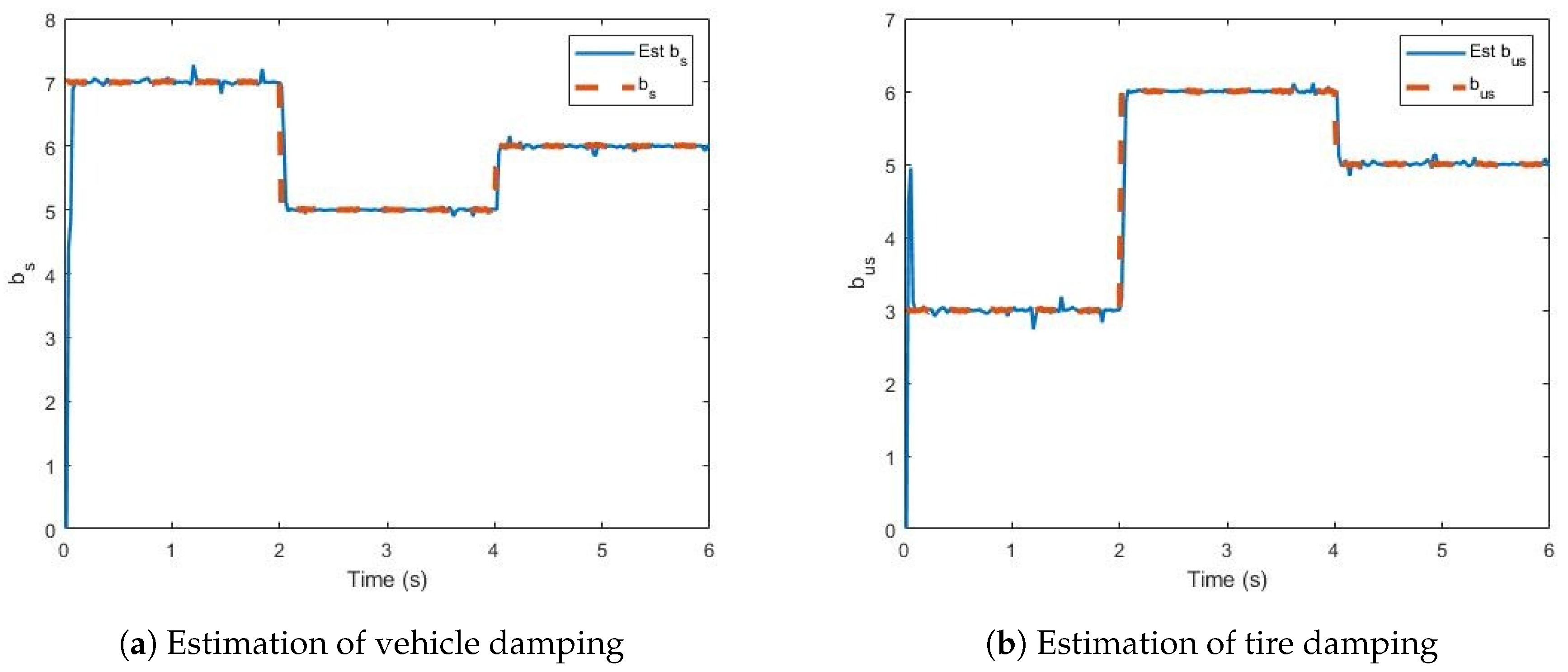
2.3. Online Estimation

In real-life applications, the parameters of the active suspension vary with time. Therefore, for more realistic investigation, the controller after training is tested without accurate knowledge of the parameters of the car body damper $b_s$ and the damping of the tire $b_{us}$, and we estimated them iteratively using the recursive least squares with exponential forgetting method, which works well with time-varying parameters [20], assuming that the parameters to be determined are not constant, but the true value changes with time. Given the initial values of ${\mathit{P}}_{\mathit{o}}$ and $\widehat{\mathit{\theta }}(\mathit{t}-\mathbf{1})$, the recursive method satisfies the following Equations (6)–(8).

$$\widehat{\mathit{\theta }}\left(\mathit{t}\right)=\widehat{\mathit{\theta }}(\mathit{t}-\mathbf{1})+\mathit{K}\left(\mathit{t}\right)(\mathit{y}\left(\mathit{t}\right)-{\mathit{\phi }}^{\mathit{T}}\left(\mathit{t}\right)\widehat{\mathit{\theta }}(\mathit{t}-\mathbf{1}))$$

(6)

$$\mathit{K}\left(\mathit{t}\right)=\mathit{P}(\mathit{t}-\mathbf{1})\mathit{\phi }\left(\mathit{t}\right){(\lambda \mathit{I}+{\mathit{\phi }}^{\mathit{T}}\left(\mathit{t}\right)\mathit{P}(\mathit{t}-\mathbf{1})\mathit{\phi }\left(\mathit{t}\right))}^{-\mathbf{1}}$$

(7)

$$\mathit{P}\left(\mathit{t}\right)=(\mathit{I}-\mathit{K}\left(\mathit{t}\right){\mathit{\phi }}^{\mathit{T}})\mathit{P}(\mathit{t}-\mathbf{1})\frac{1}{\lambda }$$

(8)

where $\widehat{\mathit{\theta }}\left(\mathit{t}\right)$ is a vector that includes the estimated parameters $b_s$ and $b_{us}$ and $\mathit{K}\left(\mathit{t}\right)$ is a weighting vector that indicates how the correction and the pervious estimate should be combined. y(t) is the measured valued; in this paper, it is the true values added with noise generated from the standard normal distribution. $\phi$ is the regressor. P(t) is a matrix defined only when the matrix $\mathbf{\Phi }{\left(\mathit{t}\right)}^{\mathit{T}}\mathbf{\Phi }\left(\mathit{t}\right)$ is nonsingular where:

$$\mathbf{\Phi }{\left(\mathit{t}\right)}^{\mathit{T}}\mathbf{\Phi }\left(\mathit{t}\right)=\sum _{\mathbf{i}=\mathbf{1}}^{\mathbf{t}}\mathit{\phi }\left(\mathit{i}\right){\mathit{\phi }}^{\mathit{T}}\left(\mathit{i}\right)$$

(9)

$\mathit{I}$ is the identity matrix with a size of $nxn$, where n is the number of parameters to be determined, and $\lambda$ is a constant chosen to be 0.90. For fast convergence and to avoid singularities, the matrix P(t) is initialized as the identity matrix multiplied by 1000. We use the unsprung mass acceleration ${\ddot{x}}_{us}$ in the online estimation process as the output y(t), since it includes all the parameters to be estimated. From (1), we can obtain the following:

$${\ddot{x}}_{us}=\frac{k_s}{m_{us}}{x}_s+\frac{b_s}{m_{us}}{\dot{x}}_s-\frac{(k_s+k_{us})}{m_{us}}{x}_{us}-\frac{(b_s+b_{us})}{m_{us}}{\dot{x}}_{us}-\frac{1}{m_{us}}u+\frac{b_{us}}{m_{us}}{\dot{z}}_r+\frac{k_{us}}{m_{us}}{z}_r$$

(10)

Taking only the coefficients of the parameters to be determined as the other parameters will disappear when the error $(\mathit{y}\left(\mathit{t}\right)-{\mathit{\phi }}^{\mathit{T}}\left(\mathit{t}\right)\widehat{\mathit{\theta }}(\mathit{t}-\mathbf{1}))$ is calculated and considering that the output satisfies:

$$\mathit{y}\left(\mathit{t}\right)=\mathit{A}\left(\mathit{t}\right)\mathit{x}\left(\mathit{t}\right)$$

(11)

yield the following:

$$\mathit{A}\left(\mathit{t}\right)={\mathit{\phi }}^{\mathit{T}}\left(\mathit{t}\right)=\left[\begin{array}{cc}\frac{{\dot{x}}_s-{\dot{x}}_{us}}{m_{us}}& \frac{-{\dot{x}}_{us}}{m_{us}}\end{array}\right]$$

(12)

such that:

$$\mathit{x}\left(\mathit{t}\right)=\left[\begin{array}{c}{b}_s\\ b_{us}\end{array}\right]$$

(13)

$$\widehat{\mathit{\theta }}\left(\mathit{t}\right)=\left[\begin{array}{c}{\widehat{b}}_s\\ {\widehat{b}}_{us}\end{array}\right]$$

(14)

where the term $\mathit{y}\left(\mathit{t}\right)$ is the measured output and $\mathit{x}\left(\mathit{t}\right)$ contains the measured parameters, whereas the term $\mathit{\phi }\left(\mathit{t}\right)$ is the estimated output and $\widehat{\mathit{\theta }}\left(\mathit{t}\right)$ contains the estimated parameters.

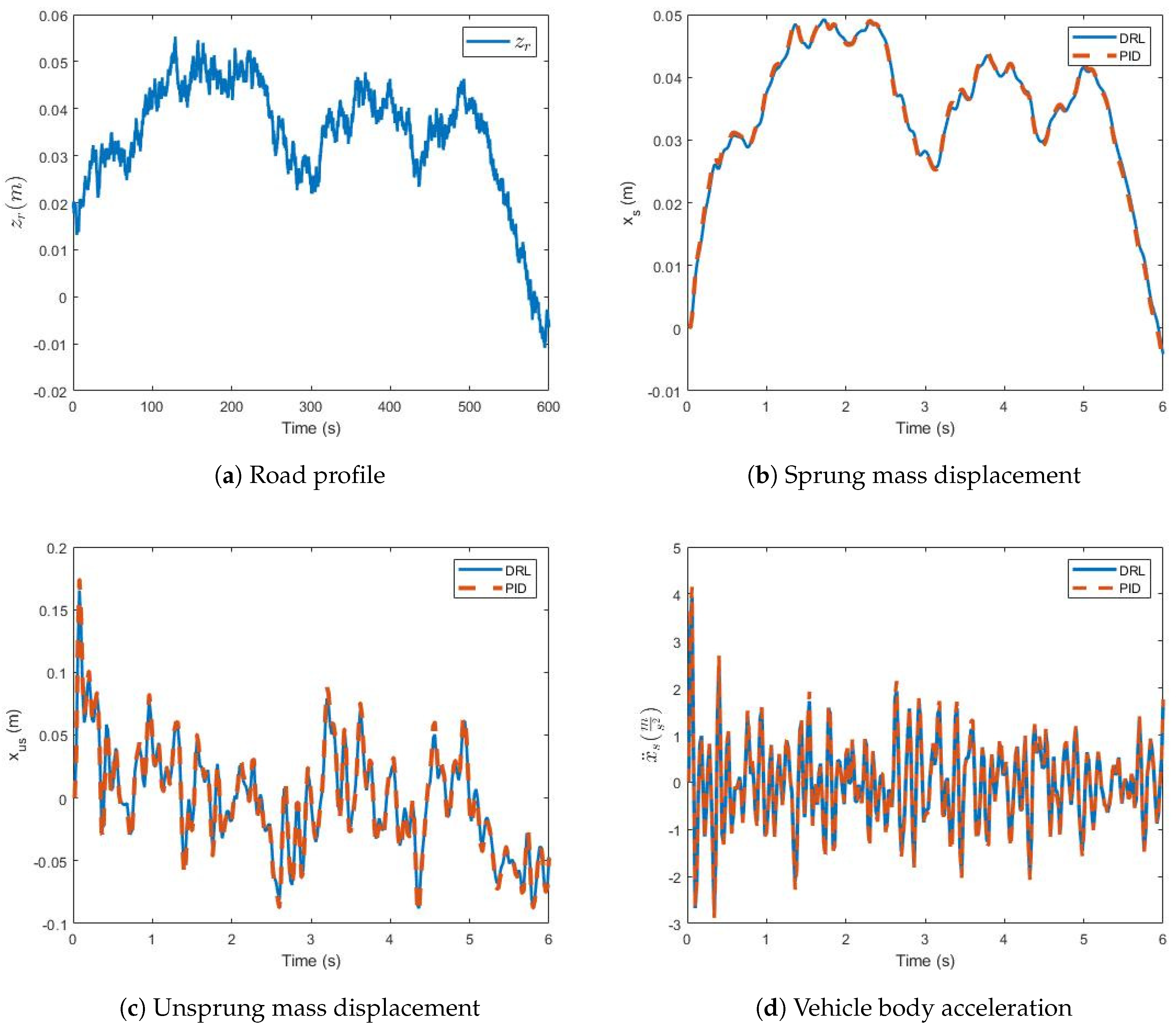
3. Results and Discussion

A simple road profile was used in the learning process where $z_r$ is generated by a square wave with an amplitude of 0.02 m and a period of 3 s, as shown in Figure 6a,b. The performance of the controller after training was compared with the optimum PID obtained from [12] and with the Linear Quadratic Regulator (LQR) from the Quanser laboratory guide [21] with the weighting matrices as follow:

$$\mathit{Q}=\left[\begin{array}{cccc}450& 0& 0& 0\\ 0& 30& 0& 0\\ 0& 0& 5& 0\\ 0& 0& 0& 0.1\end{array}\right]\mathrm{and}R=\left[0.01\right]$$

.

Two scenarios were studied to build confidence and test the trained controller. In the first scenario, the controller was compared with the optimum PID and LQR on the same road profile used during the training process under ideal conditions. In the second scenario, a new bumpy road profile was used, and parameter estimation was added to the simulation.

3.1. Scenario 1

Figure 7a–c shows the performance of the three controllers. LQR had the worst response with an overshoot of about 20% and the highest acceleration of 0.4247 m/s². The actor network and the PID performed significantly better with almost matching results. The average acceleration for the actor network and the PID was 0.2827 m/s² and 0.2919 m/s², respectively. This encouraged us to further test the actor network in new conditions and environments that were different from the training environment.

3.2. Scenario 2

The range of the road profile was extended as shown in Figure 8, and online parameter estimation was included. The new road profile is shown in Figure 8a. $b_s$ and $b_{us}$ were assumed to be changing frequently at a rate of 0.5 Hz. $b_s$ varied between 4 and 9 s/m, and $b_{us}$ varied between 3 and 7 s/m. Noise was added to the parameters to simulate noisy measurements. Figure 9a,b shows that the system successfully estimated the parameters in less than 100 ms. Despite the changing of parameters and the bumpy road profile, the actor network was able to maintain excellent performance and provided 6.14% lower overall acceleration compared to the optimum PID. The average acceleration values obtained were 0.6861 m/s² for the actor network and 0.7310 m/s² for the optimum PID.

4. Conclusions

In this paper, online reinforcement learning with the TD advantage actor critic was used to train an active suspension system controller. The structure of the neural networks was obtained by the trial and error method. Three different reward functions were studied, and the implemented one used the body vehicle velocity and the produced force as an indication of the quality of the action taken. The results showed that the reinforcement learning can obtain near optimal results under parameter uncertainty while estimating them using the RLS with forgetting factor method.

The results encourage further studies by testing other algorithms like the Deep Deterministic Policy Gradient (DDPG) and Asynchronous Advantage Actor Critic (A3C). In addition, a full model suspension system will provide a better understanding of the controller capabilities. Moreover, the adaptiveness and the ability to continuously learn the complex dynamics under disturbances and uncertainties motivate the use of deep reinforcement learning in non-linear models.

References

1. Ramsbottom, M.; Crolla, D.; Plummer, A.R. Robust adaptive control of an active vehicle suspension system. J. Automob. Eng. 1999, 213, 1–17. [Google Scholar] [CrossRef]
2. Kim, C.; Ro, P. A sliding mode controller for vehicle active suspension systems with non-linearities. J. Automob. Eng. 1998, 212, 79–92. [Google Scholar] [CrossRef]
3. Ekoru, J.E.; Dahunsi, O.A.; Pedro, J.O. Pid control of a nonlinear half-car active suspension system via force feedback. In Proceedings of the IEEE Africon’11, Livingstone, Zambia, 13–15 September 2011; pp. 1–6. [Google Scholar]
4. Talib, M.H.A.; Darns, I.Z.M. Self-tuning pid controller for active suspension system with hydraulic actuator. In Proceedings of the 2013 IEEE Symposium on Computers & Informatics (ISCI), Langkawi, Malaysia, 7–9 April 2013; pp. 86–91. [Google Scholar]
5. Salem, M.; Aly, A.A. Fuzzy control of a quarter-car suspension system. World Acad. Sci. Eng. Technol. 2009, 53, 258–263. [Google Scholar]
6. Mittal, R. Robust pi and lqr controller design for active suspension system with parametric uncertainty. In Proceedings of the 2015 International Conference on Signal Processing, Computing and Control (ISPCC), Waknaghat, India, 24–26 September 2015; pp. 108–113. [Google Scholar]
7. Ghazaly, N.M.; Ahmed, A.E.N.S.; Ali, A.S.; El-Jaber, G. H∞ control of active suspension system for a quarter car model. Int. J. Veh. Struct. Syst. 2016, 8, 35–40. [Google Scholar] [CrossRef]
8. Huang, S.; Lin, W. A neural network based sliding mode controller for active vehicle suspension. J. Automob. Eng. 2007, 221, 1381–1397. [Google Scholar] [CrossRef]
9. Heidari, M.; Homaei, H. Design a pid controller for suspension system by back propagation neural network. J. Eng. 2013, 2013, 421543. [Google Scholar] [CrossRef] [Green Version]
10. Zhao, F.; Dong, M.; Qin, Y.; Gu, L.; Guan, J. Adaptive neural networks control for camera stabilization with active suspension system. Adv. Mech. Eng. 2015, 7. [Google Scholar] [CrossRef]
11. Qin, Y.; Xiang, C.; Wang, Z.; Dong, M. Road excitation classification for semi-active suspension system based on system response. J. Vib. Control 2018, 24, 2732–2748. [Google Scholar] [CrossRef]
12. Konoiko, A.; Kadhem, A.; Saiful, I.; Ghorbanian, N.; Zweiri, Y.; Sahinkaya, M.N. Deep learning framework for controlling an active suspension system. J. Vib. Control 2019, 25, 2316–2329. [Google Scholar] [CrossRef]
13. Gordon, T.; Marsh, C.; Wu, Q. Stochastic optimal control of active vehicle suspensions using learning automata. J. Syst. Control Eng. 1993, 207, 143–152. [Google Scholar] [CrossRef]
14. Marsh, C.; Gordon, T.; Wu, Q. Application of learning automata to controller design in slow-active automobile suspensions. Veh. Syst. Dyn. 1995, 24, 597–616. [Google Scholar] [CrossRef]
15. Frost, G.; Gordon, T.; Howell, M.; Wu, Q. Moderated reinforcement learning of active and semi-active vehicle suspension control laws. J. Syst. Control Eng. 1996, 210, 249–257. [Google Scholar] [CrossRef]
16. Bucak, İ.Ö.; Öz, H.R. Vibration control of a nonlinear quarter-car active suspension system by reinforcement learning. Int. J. Syst. Sci. 2012, 43, 1177–1190. [Google Scholar] [CrossRef]
17. Chen, H.C.; Lin, Y.C.; Chang, Y.H. An actor-critic reinforcement learning control approach for discrete-time linear system with uncertainty. In Proceedings of the 2018 International Automatic Control Conference (CACS), Taoyuan, Taiwan, 4–7 November 2018; pp. 1–5. [Google Scholar]
18. Mnih, V.; Kavukcuoglu, K.; Silver, D.; Graves, A.; Antonoglou, I.; Wierstra, D.; Riedmiller, M. Playing atari with deep reinforcement learning. arXiv 2013, arXiv:1312.5602. [Google Scholar]
19. Kingma, D.P.; Ba, J. Adam: A method for stochastic optimization. arXiv 2014, arXiv:1412.6980. [Google Scholar]
20. Åström, K.J.; Wittenmark, B. Adaptive Control; Courier Corporation: North Chelmsford, MA, USA, 2013. [Google Scholar]
21. Apkarian, J.; Abdossalami, A. Active Suspension Experiment for Matlabr/Simulinkr Users—Laboratory Guide; Quanser Inc.: Markham, ON, Canada, 2013. [Google Scholar]
Figure 1. Quarter model.
Applsci 10 08060 g001
Figure 2. RL process.
Applsci 10 08060 g002
Figure 3. Critic structure.
Applsci 10 08060 g003
Figure 4. Actor structure.
Applsci 10 08060 g004
Figure 5. Algorithm implementation.
Applsci 10 08060 g005
Figure 6. Scenario 1 road profile.
Applsci 10 08060 g006
Figure 7. Scenario 1 results.
Applsci 10 08060 g007
Figure 8. Scenario 2.
Applsci 10 08060 g008
Figure 9. Parameter estimation results.
Applsci 10 08060 g009