P-Wave Reflection Approximation of a Thin Bed and Its Application

Abstract

“Thin-bed” reservoirs have become important targets of seismic exploration and exploitation. However, traditional amplitude versus offset/amplitude versus angle (AVO/AVA) technologies, for example, those based on Zoeppritz equations and their approximations for a single interface, are not sufficiently accurate for thin-bed stratigraphy. Analytic solutions of thin-bed reflectivity may become practical for thin-bed AVO analysis and inversion. Therefore, a linear analytic approximation of thin-bed P-wave reflectivity is developed under small-incidence and thin-bed assumptions. Numerical simulations show that the amplitude approximation errors are usually smaller than 10% for incidence angles less than 20 degrees, and the thin-bed thicknesses are less than one-tenth of the P-wave wavelength. Based on the least-squares approach, the inversion strategy is proposed using the approximate formula. A synthetic data test shows that the proposed inversion method can produce more accurate thin-bed properties than that based on the Zoeppritz equations, which reveals the potential of the inversion method based on the linear analytic approximate formula in the fine characterization of thin reservoirs.

1. Introduction

A large percentage of oil and gas reservoirs exist as thin beds, as their thicknesses are below seismic resolution [1]. Studies show that thin-bed amplitude versus offset/amplitude versus angle (AVO/AVA) responses depend on the thin-bed thickness and may differ significantly from that of a single interface [2,3]. Therefore, traditional AVO/AVA analysis and inversion methods, which are based on Zoeppritz equations for a single interface, are ineffective for thin-bed seismic simulation and inversion. The main problem associated with thin beds is the interference effects of all the reflecting waveforms, including converted waves and multiples.

Thin-bed reflection/transmission (R/T) coefficients in isotropic media have been studied for several decades, with discussions mainly focused on the relationship between thin-bed reflections and thickness [4,5,6,7,8,9,10]. For the cases of arbitrary incidence, Thomson [11], Haskell [12] and Brekhovskikh [13] studied reflections and transmissions of layered elastic media and provided solutions with matrix propagation. However, the complexity of their propagator matrix limited its application. Meissner and Meixner [14] and Juhlin and Young [3] presented a time-delayed R/T method and deduced that thin-bed reflections were the total stack responses of primary reflections at the top interface and the intra-bed multiples time-delayed to the primary reflection. Yang et al. [15] gave three types of approximate analytical formulas for thin-bed PP-wave reflectivity based on the work of Juhlin and Young [3] by ignoring converted waves and intra-bed multiples. Kennett et al. [16] and Kennett [17] built up the reflection and transmission matrices recursively by starting at the top interface and working down through the successive interfaces iteratively. Liu and Schmitt [10] gave an analytical formula of thin-bed seismic responses in acoustic media by ignoring multiple waves. Rubino and Velis [18] extended the work of Liu and Schmitt [10] into elastic media and used amplitude spectra to achieve thin-bed pre-stack spectral inversion. Pan and Kristopher [19] utilized Brekhovskikh’s layered elastic medium theory to develop a three-layer case and pointed out that thin-bed effects are significantly different in elastic media than in acoustic media, especially for small incidence angles.

The authors mentioned above gave a clear description of thin-bed responses. However, their thin-bed R/T coefficient formulas for arbitrary incidence are generally too complex for applications or have insufficient accuracy in that they disregarded the effects of thin-bed intra-bed multiples and converted waves. Yang et al. [20] gave thin-bed true R/T coefficients defined by displacement and approximated them to be in a quasi-Zoeppritz matrix form under the thin-bed assumption. After that, they [21] gave second-order series approximation for PP-wave reflection of a thin bed and estimated thin-bed properties, including a P-wave impedance ratio and thickness by statistical data. Considering that analytic approximations of reflection coefficients are important in AVO analysis and inversion for a single interface [22,23], we further simplify second-order series approximation under a thin-bed assumption for thin-bed AVO/AVA analysis and inversion in this paper.

First, we give a P-wave reflected approximation of a thin bed under a thin-bed assumption based on second-order series approximation. Then, we test the accuracy of the linear analytic approximation in this paper derived through numerical simulations of four representative thin-bed models. Finally, we exhibit the applicability of our approximate formula in thin-bed inversion of synthetic seismic data.

2. Theory

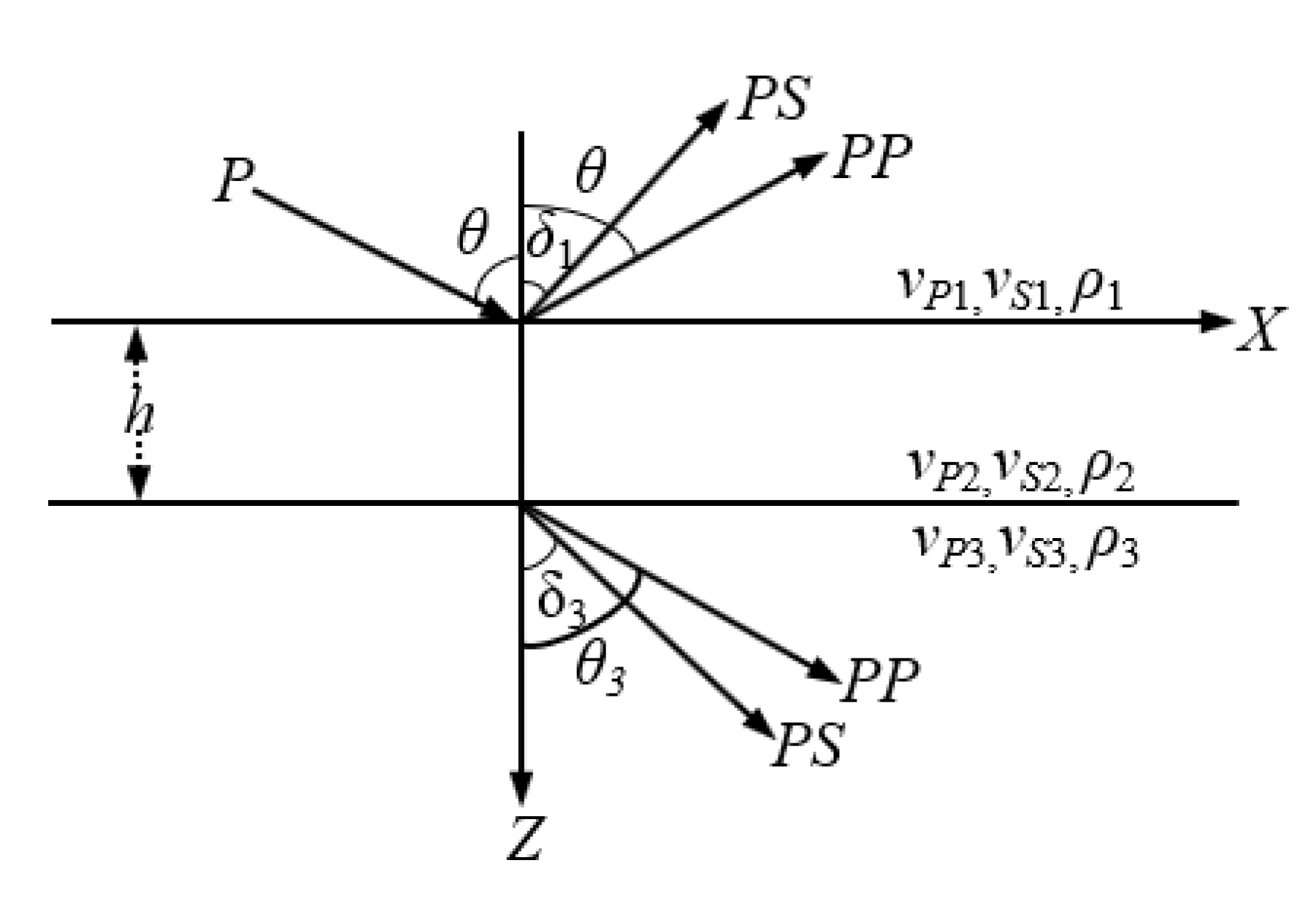
2.1. P-Wave Reflected Approximation of a Thin Bed

For a thin bed in elastic isotropic media, as shown in Figure 1, Yang et al. [21] gave second-order series approximation for P-wave reflection as follows,

$$R_{PP}\approx A_0+A_2{\sin }^2\theta ,$$

(1)

where θ is incidence angle, A₀ and A₂ are the intercept and gradient, respectively, which are presented in Appendix A in detail.

When the middle layer’s thickness h is ultrathin, then ωh/v_P2 << 1 and ωh/v_S2 << 1, which are defined as τ and q, respectively, in Equation (1) (shown in Appendix A). That is, τ << 1 and q << 1. Using first-order Taylor expansions,

$$\sin \tau \approx \tau ,\sin q\approx q,\cos \tau \approx 1,\cos q\approx 1,$$

(2)

Equation (1) is simplified as

$$R_{PP}\approx P+G{\sin }^2\theta ,$$

(3)

with

$$P=\frac{1}{n_0}\left(\frac{z_{P3}}{z_{P1}}-1\right)+\frac{j\tau }{n_0}\left(\frac{z_{P2}}{z_{P1}}-\frac{z_{P3}}{z_{P2}}\right),$$

(4)

$$\begin{array}{ll}G=\frac{1}{2n_0}& \left(\frac{z_{P3}}{z_{P1}}+j\tau \frac{z_{P2}}{z_{P1}}+\frac{4j\tau l_1}{r_1^2}\right)\left(P+\frac{2}{r_1}A-1\right)+\frac{l_1{l}_2}{n_0{r}_3}\left(1-\frac{2}{r_3}\right)\frac{z_{P3}}{z_{P1}}B\\ & +\frac{1}{n_0}\left[\frac{2}{r_1^2}+j\tau \left(l_1-\frac{2l_1}{r_2^2}+\frac{2}{r_1^2}\frac{z_{P1}}{z_{P2}}\right)\frac{z_{P3}}{z_{P1}}\right]\left(1+P+A\right)\\ & +\frac{j\tau l_1}{n_0{r}_1}\left(1-\frac{4}{r_1^2}\right)A+\frac{l_1^2{l}_2^2}{n_0}\left(\frac{1}{2}-\frac{2}{r_3^2}\right)\frac{z_{P3}}{z_{P1}}\frac{2}{n_0}\left(1+{\tau }^2\right)\end{array}$$

(5)

Other parameters are presented in Appendix B in detail.

Equation (3) is the linear analytic approximation of a thin-bed P-wave reflection coefficient. The approximate formula is written as a sum of the constant term and the first order term of the sine-squared incidence angle. Compared with Equation (1), the linear analytic approximation has a relatively compact form (shown in Appendix A and Appendix B), which is more convenient to achieve AVO/AVA analysis and inversion of a thin bed.

Compared with linearized approximations to the Zoeppritz equations for a single interface [22,23,24], the intercept and gradient of the linear analytic approximation for the thin-bed P-wave reflectivity are frequency dependent; furthermore, they are functions of elastic parameters of the target thin bed and the upper and lower half spaces. Meanwhile, the linear analytic approximation is derived with no weak impedance contrast hypothesis, so it is valid for thin-bed models with strong impedance contrasts, such as coal seams, etc.

2.2. Inversion of Thin-Bed Elastic Parameters and Thickness

Based on the linear analytic approximation, we invert for elastic parameters and thickness of the thin-bed reservoir, including P- and S-wave velocities and densities of the target thin bed and its upper and lower half spaces and thin-bed thickness. The inversion procedure of thin-bed properties is as follows.

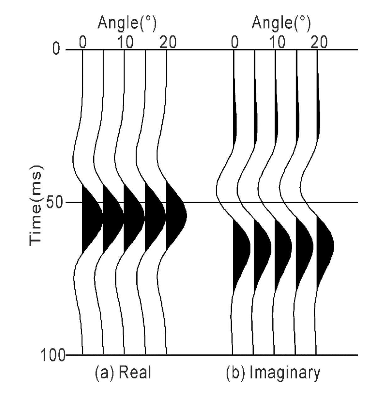
2.2.1. Extraction of Complex Reflection Coefficients

Because thin-bed reflection coefficients are complex valued and frequency dependent, we construct complex seismic trace and analyze it in the frequency domain. The conventional AVA seismic trace s^real(θ,t) of a thin bed is viewed as the real component of thin-bed complex trace. The imaginary component s^im(θ,t) can be calculated through Hilbert transform [25,26,27]:

$$s^{im}\left(\theta ,t\right)=s^{real}\left(\theta ,t\right)\ast \frac{1}{\pi t}$$

(6)

where the symbol * is time convolution.

The complex AVA trace s(θ,t) in the time domain is:

$$s\left(\theta ,t\right)=s^{real}\left(\theta ,t\right)+j{s}^{im}\left(\theta ,t\right),$$

(7)

where j is the imaginary term. s(θ,t) in the frequency domain can be obtained through Fourier transform:

$$S\left(\theta ,f\right)=\mathrm{FFT}\left[s\left(\theta ,t\right)\right].$$

(8)

If the seismic wavelet w(θ,t) in the time domain is known, we can calculate its value in the frequency domain through Fourier transform:

$$W\left(\theta ,f\right)=\mathrm{FFT}\left[w\left(\theta ,t\right)\right].$$

(9)

Thus, the reflection coefficients of a thin bed in the frequency domain can be derived by:

$$R^{obs}\left(\theta ,f\right)=S\left(\theta ,f\right)/W\left(\theta ,f\right),$$

(10)

where R^obs(θ,f) is the observed reflection coefficient matrix of an AVA dataset at different frequencies.

If the seismic wavelet is not known, Liu et al. [28] gave a method to estimate the reflection coefficient from seismic data for a single-interface case. We can extend Liu’s method to estimate R^obs by extracting its real and imaginary components from those of AVA traces, respectively.

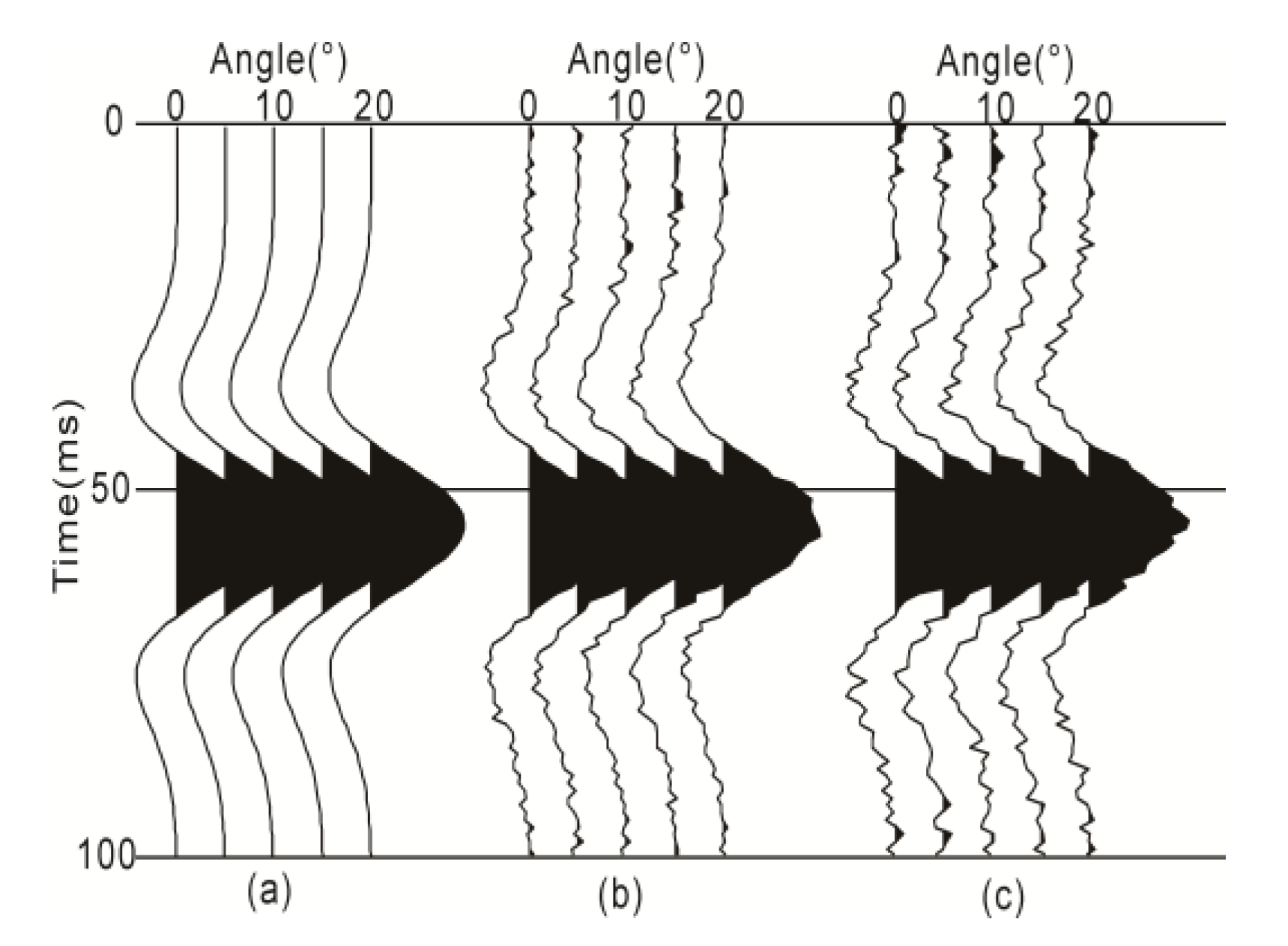
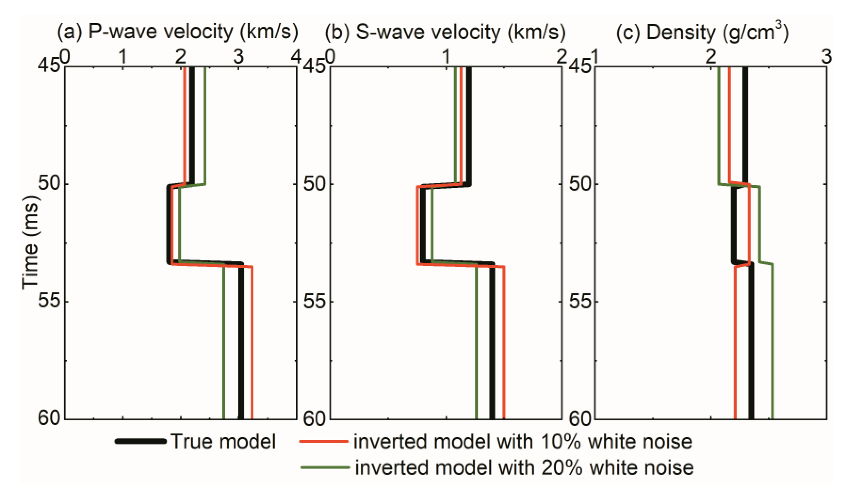
2.2.2. AVA Inversion of Thin-Bed Properties

According to a least-squares approach, the objective function Q for the inversion of the thin-bed P-wave reflection coefficient is defined as follows:

$$Q\left(m\right)={\Vert R^{obs}-R\Vert }^2,$$

(11)

where m = (v_P vs. ρ h)^T are the thin-bed elastic parameters and thickness. R is the vector of the calculated P-wave reflection coefficients by the linear analytic approximation for the given model parameter vector m. The update model vector Δm = (Δv_P Δv_S Δρ Δh)^T can be calculated through the Gauss–Newton formula [29,30,31,32] as:

$$\Delta m={\left[J^T\left(m\right)J\left(m\right)+\chi I\right]}^{-1}{J}^T\left(m\right)\left[R\left(m_0+\Delta m\right)-R\left(m_0\right)\right],$$

(12)

where m₀ is the initial parameter vector, χ is a Lagrange multiplier, I is an identity matrix and J is the Jacobian matrix as

$$J=\left[\frac{\partial R_i\left(m\right)}{\partial m_k}\right]\mathrm{with}i=1,\dots ,NA\times NF;k=1,\dots ,NM,$$

(13)

where the subscripts i, k indicate indices for reflection coefficients and model parameters, respectively; NA, NF and NM are the numbers of angle, frequency and model parameters, respectively.

Considering that m has many parameters, including P-wave velocities, S-wave velocities, densities of three layers and the thickness of middle layer for a thin bed, t is more prone to obtaining local minimum solutions than conventional AVA inversion. In order to obtain reasonable inversion results, priori information is adopted to constraint the inverted thin-bed model.

3. Numerical Analysis and Application

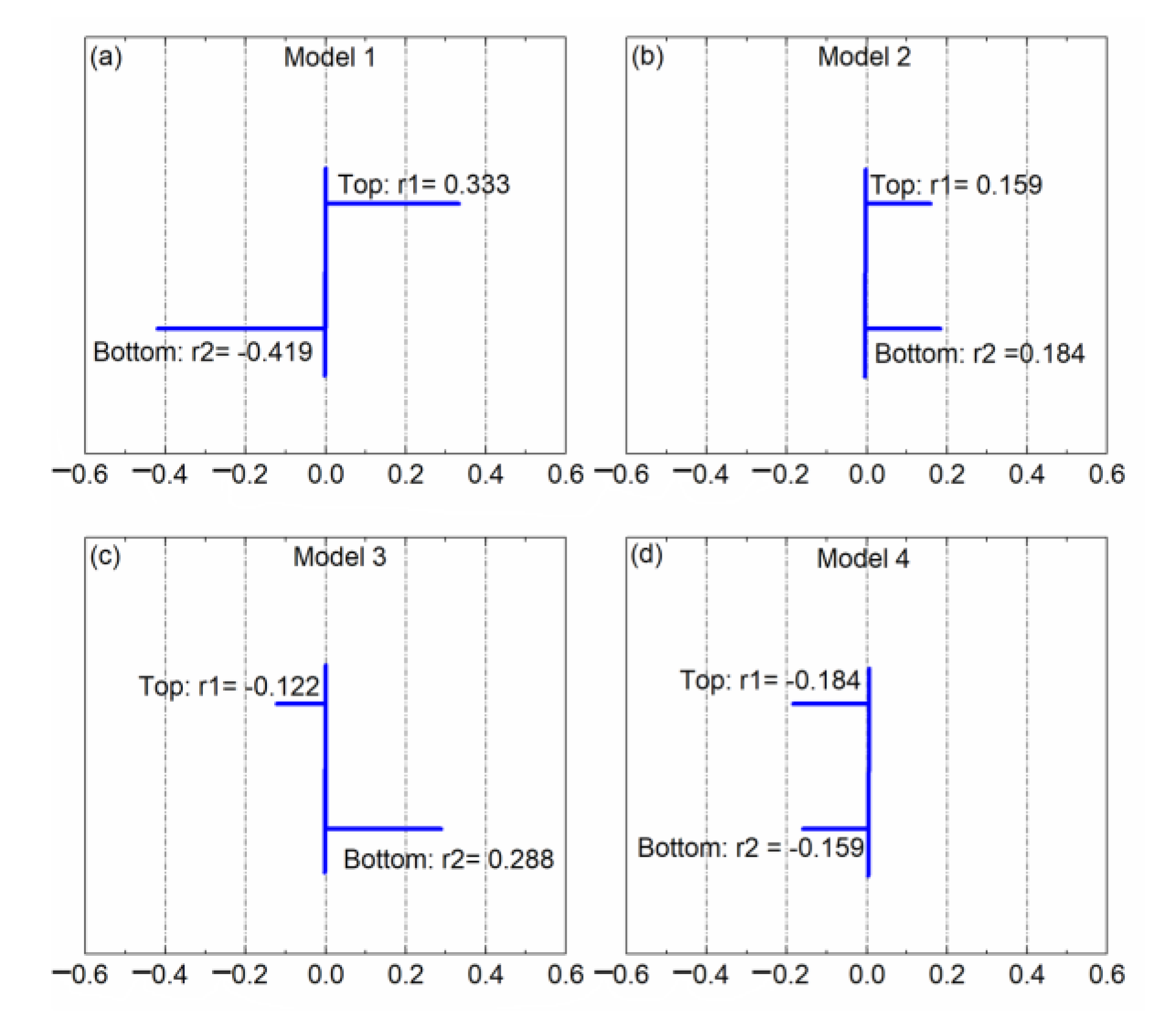
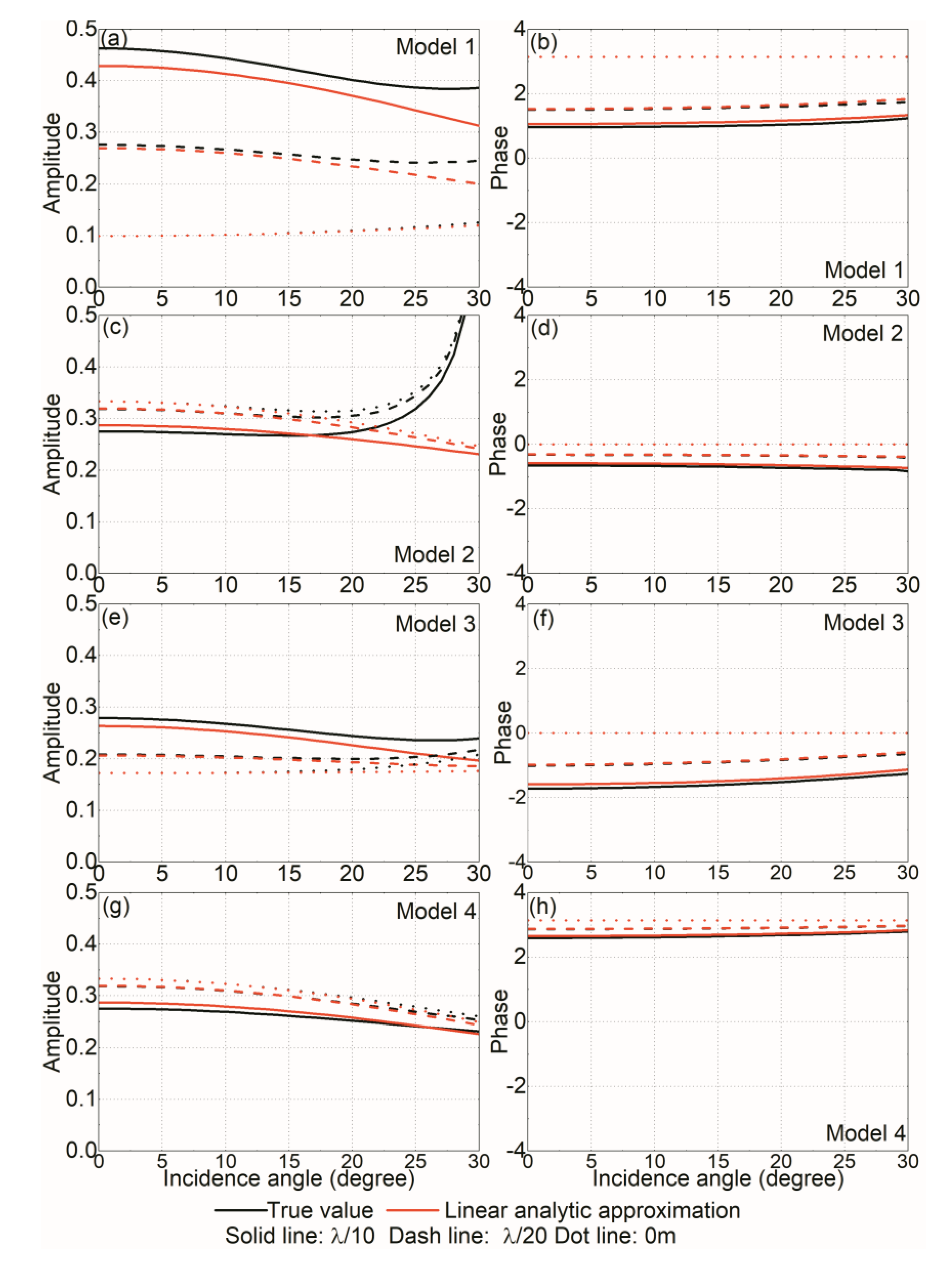
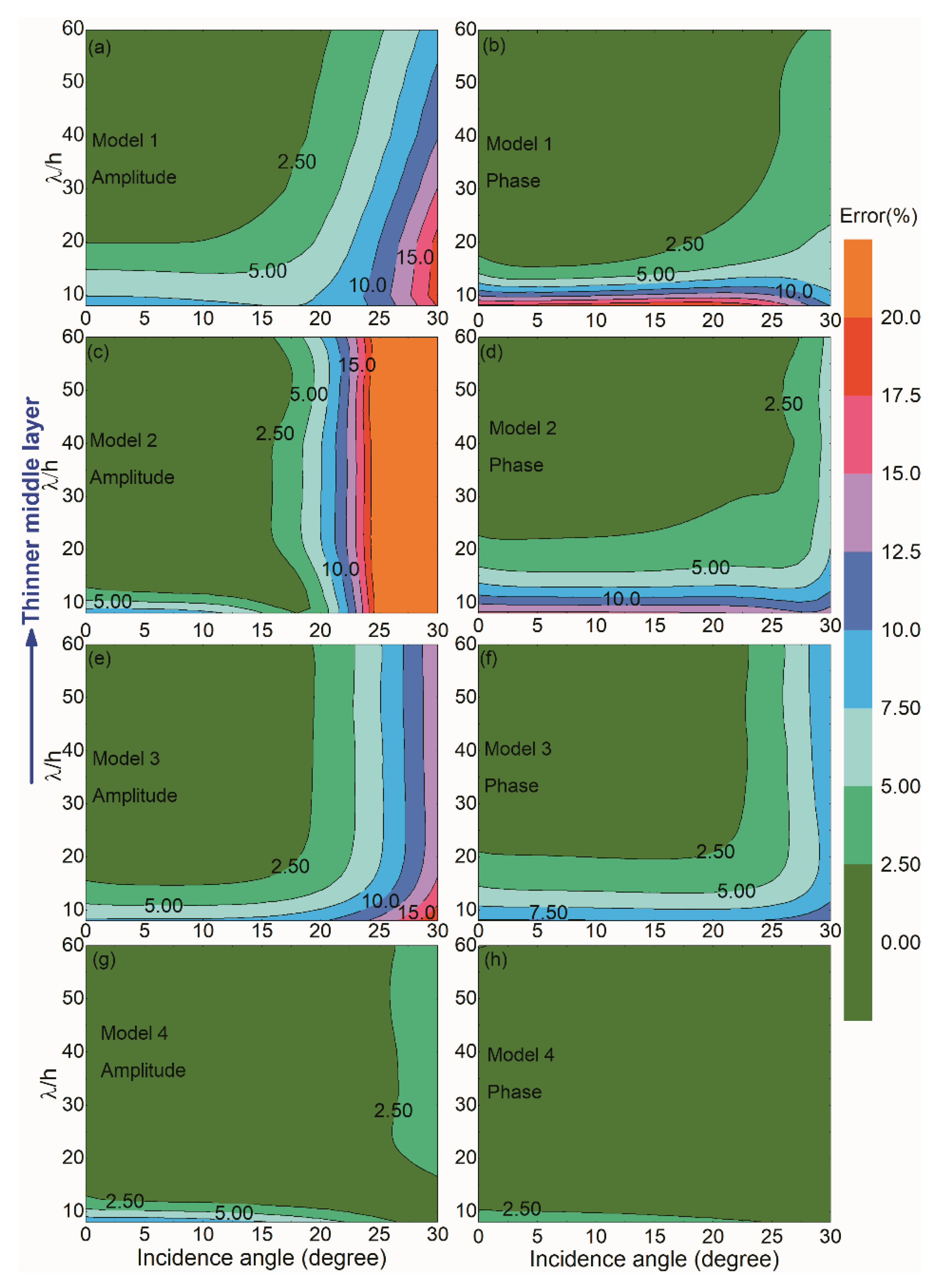
3.1. Approximation Accuracy Analysis

In order to verify the accuracy of the linear analytic approximation of the thin-bed P-wave reflection coefficient derived in this paper, we conduct tests on four representative thin-bed models, including: (1) high-impedance thin bed, (2) low-to-high impedance transition layers, (3) low-impedance thin bed and (4) high-to-low impedance transition layers [10,33].

Table 1. Parameters of thin-bed models. I_P and I_S are P-wave and S-wave impedances, respectively, units of velocities and densities in Table 1 are m/s and g/cm³, respectively.

	Layer No.	vP	vS	ρ	IP	IS
Model 1	1	3050	1525	2.7	8235	4117.5
	2	6100	3050	2.7	16,470	8235
	3	2500	1525	2.7	6750	4117.5
Model 2	1	3050	1600	2.7	8235	4320
	2	4200	2500	2.7	11,340	6750
	3	6100	3100	2.7	16,470	8370
Model 3	1	2200	1200	2.3	5060	2760
	2	1800	800	2.2	3960	1760
	3	3050	1400	2.35	7167.5	3290
Model 4	1	6100	3100	2.7	16,470	8370
	2	4200	2500	2.7	11,340	6750
	3	3050	1600	2.7	8235	4320

lists the elastic parameters and Figure 2 plots the reflectivity logs of these four models. Figure 2 shows that Models 1 and 3 produce opposite-polarity reflections, while Models 2 and 4 produce identical-polarity reflections. Compared with Models 2–4, Model 1 has stronger impedance contrasts, which are utilized to test the approximate formula’s applicability in thin-bed models with strong impedance contrasts. In the numerical simulations, we set thin-bed thicknesses as λ/8, λ/10, λ/20, λ/30, λ/40, λ/50 and λ/60, where λ is the P-wavelength in the target thin bed. Considering the small-incidence assumption, the incidence angle in all cases is set from 0 degree to 30 degrees with a 1-degree sample interval.

For a better understanding of the behavior of the linear analytic approximate formula, we compare the linear analytic approximation and the true value of thin-bed P-wave reflection coefficients [20] by illustrating λ/10 and λ/20 examples, as shown in Figure 3. In order to prove that the parameters P and G are derived accurately, the cases of thin-bed thicknesses equal to zero, i.e., single-interface cases, are also shown in Figure 3. The absolute values of relative errors are plotted in Figure 4. Thin-bed PP-wave reflection coefficients are complex valued. Therefore, we discuss thin-bed P-wave reflection coefficients in terms of their amplitude and phase sections, which are shown in Figure 3 and Figure 4.

Figure 3 shows the P-wave reflection coefficients as a function of incidence angle for Models 1–4 for only three of the modeled cases, λ/10, λ/20 and 0 m. As models with opposite-polarity reflections, Models 1 and 3 share similar regularity. In the angle range from 0 to 20 degrees, the linear analytic approximation demonstrates the same AVA gradient, but a lower AVA intercept, compared to the true PP-wave response. For incidence angles greater than 20 degrees, the linear analytic approximation starts to diverge further from the true value. An explanation for this behavior is that the linear analytic approximation relies on the small-incidence assumption. As models with identical-polarity reflections, Models 2 and 4 share similar regularity only for incidence angles smaller than 20 degrees. For Model 2 with a 30-degree critical angle, the AVA curves of the linear analytic approximation diverge further from the true value with increasing angle over 20 degrees. Especially near the critical angle, the true P-wave reflection coefficient increases sharply, while the linear analytic approximation becomes invalid. For Model 4 with no critical angles, the linear analytic approximation is nearly the same as the true values. Comparison of the λ/10 and λ/20 cases shows that a thinner bed results in a higher accuracy for amplitude and phase responses of the linear analytic approximation. For single-interface cases, the true equations of thin-bed R/T coefficients are simplified into Zoeppritz equations [20]. Approximate amplitudes are coincident with the true amplitudes for incidence angles less than 20 degrees. Meanwhile, approximate phases are zero or pi, which are equal to the true phases. The high accuracy of approximate values for single-interface cases confirms that derivations of the parameters P and G are accurate.

Figure 4 shows errors in amplitude (left) and phase (right) caused by the linear analytic approximation for Models 1–4 with incidence angles for the full range of λ/h cases tested. Comparison between different λ/h cases for small incidence shows that approximation errors decline with a thinner bed and drop below 5% rapidly with decreasing thickness of the thin bed. For models with critical angles, i.e., Models 1–3, the relative errors versus incidence angle and thickness share a similar phenomenon. For incidence angles less than 20 degrees and thicknesses less than λ/10, the amplitude errors are less than 10%. For incidence angles greater than 20 degrees, the amplitude errors are larger than 10%, and increase with increasing incidence angle and thin-bed thickness. The amplitude errors rise quickly for incidence angles near the critical angles, and the linear analytic approximation becomes invalid. Applicability of the approximate formula for Model 1 shows that the linear analytic approximation is valid for thin-bed models with strong impedance contrasts. For model with no critical angles, i.e., Model 4, approximation errors smaller than 5% for a thickness smaller than λ/8. Compared with the Model 1–3 cases, the linear analytic approximation for Model 4 has a relatively higher accuracy, which exhibits a better applicability of the linear analytic approximation for low-to-high impedance transition layers.

From numerical tests, we can conclude that: when incidence angles are less than 20 degrees and thin-bed thicknesses are less than one-tenth of the P-wave wavelength, the approximation amplitude errors are smaller than 10%, which verifies the applicability of the linear analytic approximation.

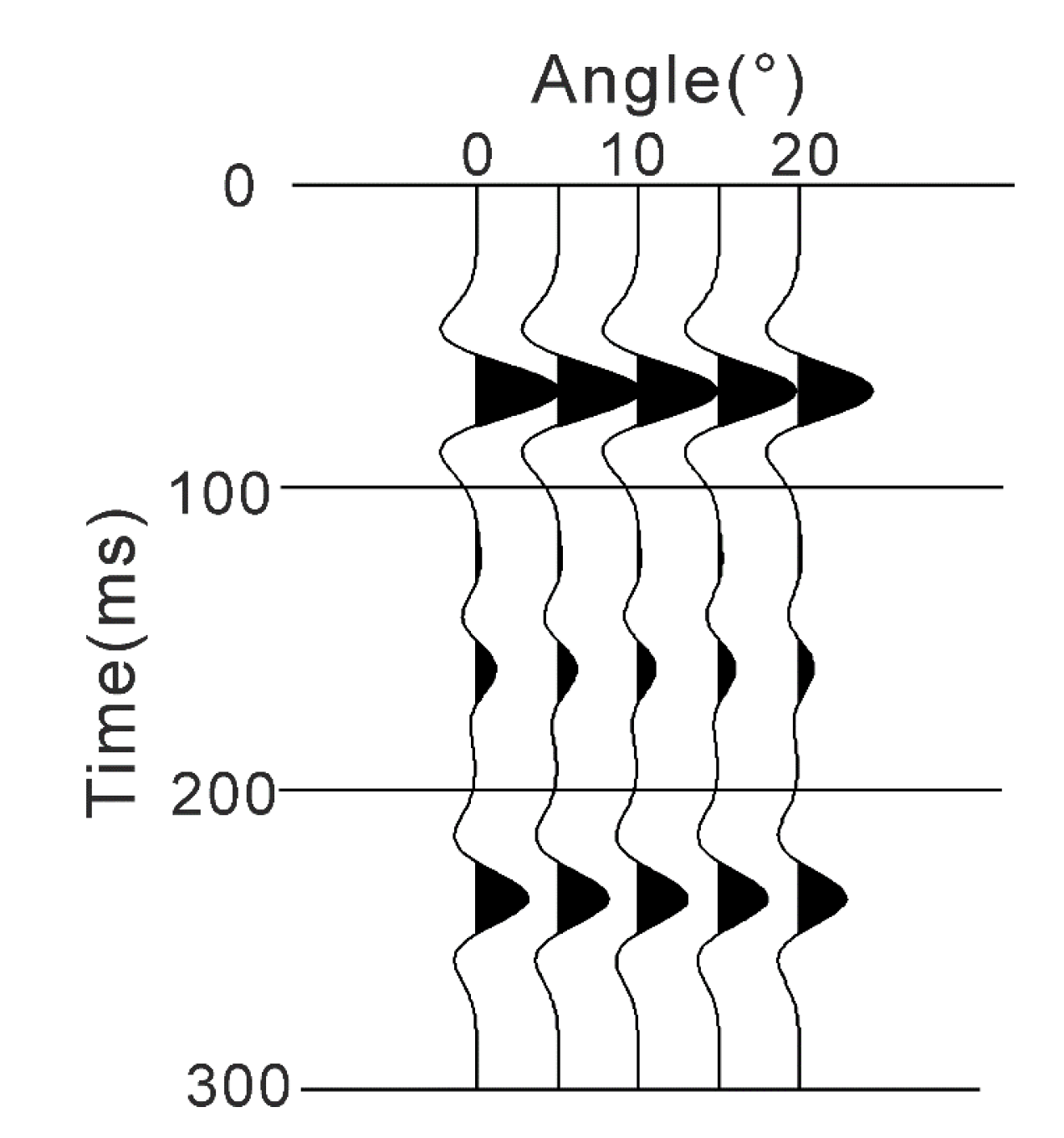
3.2. Application Examples

Using the linear analytic approximation of thin-bed P-wave reflection coefficients, thin-bed elastic parameters and thickness are inversed through a least-squares approach. We apply the proposed inversion flow to predict thin-bed properties from synthetic seismic data.

Considering that thin-bed properties of Model 3 are close to those of some actual reservoirs, such as coal seams and unconsolidated sandstone, we take Model 3 as a thin-bed model to exhibit application of the approximate formula to synthetic data in this section. Using the true P-wave reflection coefficient, we simulate the synthetic AVA records of Model 3 using the Ricker wavelet with a 25 Hz predominant frequency. The thin-bed thickness is set as 3 m and the incidence angles range from 0 to 20 degrees. Taking the synthetic AVA records as the real seismic traces, we construct complex seismic traces through the Hilbert transform, which are shown in Figure 5. Compared with the real component, the imaginary records have the same amplitude envelope but 90-degree phase shift. Thin-bed complex reflection coefficients are derived using Equation (10).

The calculation procedure of thin-bed reflection coefficients is shown in Figure 6 by taking normal responses of Model 3 as an example. Using the real and imaginary reflection coefficients, we invert for thin-bed properties by the proposed thin-bed inversion method and by the conventional AVA inversion method based on the Zoeppritz equations. As shown in Figure 7, the proposed thin-bed inversion method is superior in the characterization of thin-bed properties compared to the conventional AVA inversion method. The proposed thin-bed inversion method can derive more accurate elastic parameters of the target thin bed and its upper and lower half spaces. In particular, the inversion results can indicate the thickness of the target thin bed clearly and accurately.

In order to test the influence of noise on the inversion, we add 10% (mean energy ratio) and 20% white noise to the real AVA records, which are shown in Figure 8.

The inverted results of thin-bed properties are shown in Figure 9. For 10% white noise data, it can be seen that thin-bed thickness is basically coincident with that of the true model. The inverted P-wave and S-wave velocities deviate from the true model relatively more. Compared with the P-wave and S-wave velocities, the error in the density inversion is larger. The reason is that incidence angles of our AVA gather are from 0 to 20 degrees, which are not so large. Normally, stable density inversion requires larger incidence angle gathers. Compared to the 10% white noise case, the inverted P-wave and S-wave velocities for the 20% white noise case have higher inversion errors, while they can reveal the true size relationship of thin-bed elastic parameters.

In order to test the thin-bed inversion strategy against synthetic data of multi-layer models, we set a six-layer 1D model named “Model 5”, and synthetic P-wave AVA datasets, as shown in Figure 10.

Table 2. Parameters of multi-layer models. Units of velocities, densities and thickness in Table 2 are m/s, g/cm³ and m, respectively.

	Layer No.	vP	vS	ρ	Thickness
Model 5	1	1500	700	1.80	50
	2	2400	1200	2.31	100
	3	1800	800	2.20	3
	4	2500	1250	2.32	100
	5	3000	1500	2.40	6
	6	3500	1700	2.60	∞

lists the elastic parameters and layer thicknesses of Model 5. A Ricker wavelet with a 25 Hz predominant frequency is chosen as the synthetic seismic wavelet.

Under the seismic resolution limit of a 25 Hz predominant frequency, Model 5 includes an impedance interface and two thin beds. The impedance interface is between layer 1 and layer 2, and is a low-to-high impedance interface. One thin bed is a 3 m low-impedance thin bed, which is constituted by layer 2, layer 3 and layer 4. The other thin bed is a 6 m low-to-high impedance transition layer, which is constituted by layer 4, layer 5, and layer 6. Figure 11 shows the inversion results of thin-bed properties by the proposed thin-bed inversion and those by the conventional AVA inversion [34].

For the impedance interface located at 67 ms in the time domain, the inversion results by the proposed thin-bed inversion show that the middle layer is equal to the third layer. Meanwhile, the inverted P-wave velocities and densities are very close to the true P-wave velocities and densities, respectively. Compared with the inverted results by Zoeppritz’s approximate formula, the inverted S-wave velocities diverge relatively further from the true S-wave velocities. Meanwhile, considering that thin-bed inversion needs to carry out complicated calculations in a complex domain, conventional Zoeppritz inversion is a better choice for an impedance interface. For the low-impedance thin bed located at 150 ms, compared with the conventional AVA inversion, the proposed thin-bed inversion method derives more accurate elastic parameters of the target thin bed. For the low-to-high impedance transition layers located at 233 ms, the conventional AVA inversion method cannot reveal the existence of the target thin bed. Meanwhile, the thin-bed inversion reveals the existence of the target thin bed very well. Moreover, the inverted P-wave velocities and thin-bed thicknesses are close to the true values.

4. Discussion

Compared with the reflection coefficient equations of a single interface, the thin-bed reflectivity approximation gives closer descriptions of thin-bed seismic responses. However, the approximate formula is also based on the fundamental assumptions of conventional AVO methods, such as horizontal interface, plane-wave incidence, etc. Therefore, the approximate formula is more applicable for the thin-bed reservoirs with relatively simple structures. For the inversion problems of complicated structure reservoirs, the inversion methods based on numerical solutions of wave equation are being studied and applied in depth. For example, recently, Pan et al. [35] successfully applied elastic full-waveform inversion to a field dataset for reservoir characterization. However, at present, the published papers on the thin-bed inversion based on numerical solutions of wave equation are very rare. Therefore, the approximate formula and the corresponding inversion method proposed in this paper still has potentially exploitable superiority for thin-bed AVO inversion.

This paper concentrates on the P-wave reflectivity approximation of a single thin bed. The situation becomes more complex if the target thin layer is embedded in a finely layered background. Research on finely layered reservoirs shows that the interlayer structure and lithologies can be generally determined through long-wavelength approximation [36,37,38,39,40,41]. Therefore, we will introduce long-wavelength approximation in our further AVA inversion of finely layered reservoirs.

The proposed thin-bed inversion strategy inverts for ten parameters of a thin bed, including P-wave and S-wave velocities and densities of the target thin bed and its upper and lower half spaces and thin-bed thickness. Thin-bed AVA inversion is prone to obtaining local minimum solutions due to many unknown parameters to invert. In this paper, we adopt logging information to constrain the inverted thin-bed model for reasonable inversion results. Studies on a single interface show that the parameterization method reduces the number of unknown parameters and improves the stability of single-interface inversion [42,43]. Therefore, we will introduce the parameterization method in our further AVA inversion of a thin bed for a more stable inversion.

In the tests of synthetic seismic data, we just made a preliminary attempt to do the inversion based on our formula. The noise tests show that the inversion method has a certain anti-noise ability. Moreover, we have not yet developed a mature process and program for the large-scale industrial applications of our inversion method. At present, we can only build the initial model manually and invert the AVA gathers one by one. In a future study, we will try to enhance the anti-noise capabilities of the inversion method, and develop matching data processing techniques.

5. Conclusions

This paper derives thin-bed P-wave reflectivity as a linear analytic approximation under small-incidence and thin-bed assumptions. The linear analytic approximation can be reduced to formulas in case of a single interface when the thin-bed thickness is set to zero. Numerical tests of four representative thin-bed models show that when incidence angles are less than 20 degrees and thin-bed thicknesses are less than one-tenth of the P-wave wavelength, the approximated amplitude errors are smaller than 10%. Compared to the second-order series approximation, the linear analytic approximation has a relatively compact form, which helps facilitate usage in an inversion scheme.

Using the linear analytic approximation, this paper proposes an inversion methodology of thin-bed properties (P-wave velocities, S-wave velocities, densities of the target thin bed and its overburden and underburden, as well as thin-bed thickness) from AVA gathers through a least-squares algorithm. Inversion applications to synthetic data exhibit the applicability of the linear analytic approximation in thin-bed AVA inversion.

References

1. Zeng, H.; Backus, M.M. Interpretive advantages of 90°-phase wavelets: Part 1—Modeling. Geophysics 2005, 70, C7–C15. [Google Scholar] [CrossRef]
2. Almoghrabi, H.; Lange, J. Layers and bright spots. Geophysics 1986, 51, 699–709. [Google Scholar] [CrossRef]
3. Juhlin, C.; Young, R. Implications of thin layers for amplitude variation with offset (AVO) studies. Geophysics 1993, 58, 1200–1204. [Google Scholar] [CrossRef]
4. Widess, M.B. How thin is a thin bed? Geophysics 1973, 38, 1176–1180. [Google Scholar] [CrossRef]
5. Neidell, N.S.; Poggiagliolmi, E. Stratigraphic modeling and interpretation—Geophysical principles, in Payton, C.E., Eds., Seismic stratigraphy—Application to hydrocarbon exploration. Am. Assn. Petr. Geol. Memoir 1977, 26, 389–416. [Google Scholar]
6. Koefoed, O.; De Voogd, N. The linear properties of thin layers, with an application to synthetic seismograms over coal seams. Geophysics 1980, 45, 1254–1268. [Google Scholar] [CrossRef]
7. De Voogd, N.; Rooijen, H.D. Thin-layer response and spectral bandwidth. Geophysics 1983, 48, 12–18. [Google Scholar] [CrossRef]
8. Chung, H.; Lawton, D.C. Amplitude responses of thin beds: Sinusoidal approximation versus Ricker approximation. Geophysics 1995, 60, 223–230. [Google Scholar] [CrossRef]
9. Chung, H.M.; Lawton, D.C. Frequency characteristics of seismic reflections from thin beds. Can. J. Explor. Geophys. 1995, 31, 32–37. [Google Scholar]
10. Liu, Y.; Schmitt, D.R. Amplitude and AVO responses of a single thin bed. Geophysics. 2003, 68, 1161–1168. [Google Scholar] [CrossRef]
11. Thomson, W.T. Transmission of Elastic Waves through a Stratified Solid Medium. J. Appl. Phys. 1950, 21, 89–93. [Google Scholar] [CrossRef]
12. Haskell, N.A. The dispersion of surface waves on multilayered media. In Vincit Veritas: A Portrait of the Life and Work of Norman Abraham Haskell; Wiley: New Jersey, NJ, USA, 1990; pp. 86–103. [Google Scholar] [CrossRef]
13. Brekhovskikh, L.M. Waves in Layered Media; Academic Process: Tamil Nadu, India, 1960. [Google Scholar]
14. Meissner, R.; Meixner, E. Deformation of seismic wavelets by thin layers and layered boundaries. Geophys. Prospect. 1969, 17, 1–27. [Google Scholar] [CrossRef]
15. Yang, C.; Wang, Y.; Lu, J. Weak impedance difference approximations of thin-bed PP-wave reflection responses. J. Geophys. Eng. 2017, 14, 1010–1019. [Google Scholar] [CrossRef]
16. Kennett, B.L.N.; Kerry, N.J.; Woodhouse, J.H. Symmetries in the reflection and transmission of elastic waves. Geophys. J. Int. 1978, 52, 215–229. [Google Scholar] [CrossRef]
17. Kennett, B.L.N. Seismic Wave Propagation in a Stratified Medium; Cambridge University Press: Cambridge, UK, 1983. [Google Scholar]
18. Rubino, J.G.; Velis, D. Thin-bed pre-stack spectral inversion. Geophysics 2009, 74, R49–R57. [Google Scholar] [CrossRef]
19. Pan, W.; Innanen, K.A. AVO/AVF analysis of thin beds in elastic media. SEG Tech. Program Expand. Abstr. 2013, 2013, 373–377. [Google Scholar]
20. Yang, C.; Wang, Y.; Wang, Y. Reflection and transmission coefficients of a thin bed. Geophysics 2016, 81, N31–N39. [Google Scholar] [CrossRef] [Green Version]
21. Yang, C.; Wang, Y.; Lu, J.; Chen, B.; Shi, L. A Low-Order Series Approximation of Thin-Bed PP-Wave Reflections. Appl. Sci. 2019, 9, 709. [Google Scholar] [CrossRef] [Green Version]
22. Aki, K.; Richards, P.G. Quantitative Seismology—Theory and Methods; W.H. Freeman and Co: New York, NY, USA, 1980. [Google Scholar]
23. Shuey, R.T. A simplification of the Zoeppritz equations. Geophysics 1985, 50, 609–614. [Google Scholar] [CrossRef]
24. Smith, G.; Gidlow, P. Weighted stacking for rock property estimation and detection of gas. Geophys. Prospect. 1987, 35, 993–1014. [Google Scholar] [CrossRef]
25. Taner, M.T.; Koehler, F.; Sheriff, R.E. Complex seismic trace analysis. Geophysics 1979, 44, 1041–1063. [Google Scholar] [CrossRef]
26. Robertson, J.D.; Nogami, H.H. Complex seismic trace analysis of thin beds. Geophysics 1984, 49, 344–352. [Google Scholar] [CrossRef]
27. Barnes, A.E. Theory of 2-D complex seismic trace analysis. Geophysics 1996, 61, 264–272. [Google Scholar] [CrossRef]
28. Liu, Y.; Tinivella, U.; Liu, X. An inversion method for seafloor elastic parameters. Geophysics 2015, 80, N11–N21. [Google Scholar] [CrossRef]
29. Levenberg, K. A method for the solution of certain non-linear problems in least squares. Q. Appl. Math. 1944, 2, 164–168. [Google Scholar] [CrossRef] [Green Version]
30. Marquardt, D.W. An algorithm for least-squares estimation of non-linear inequalities. J. Soc. Ind. Appl. Math. 1963, 11, 431–441. [Google Scholar]
31. Lu, J.; Yang, Z.; Wang, Y.; Shi, Y. Joint PP and PS AVA seismic inversion using exact Zoeppritz equations. Geophysics 2015, 80, R239–R250. [Google Scholar] [CrossRef] [Green Version]
32. Lu, J.; Wang, Y.; Chen, J. Detection of Tectonically Deformed Coal Using Model-Based Joint Inversion of Multi-Component Seismic Data. Energies 2018, 11, 829. [Google Scholar] [CrossRef]
33. Chen, T.; Liu, Y. Multi-component AVO response of thin beds based on reflectance spectrum theory. Appl. Geophys. 2006, 3, 27–36. [Google Scholar] [CrossRef]
34. Fatti, J.L.; Smith, G.C.; Vail, P.J.; Strauss, P.J.; Levitt, P.R. Detection of gas in sandstone reservoirs using AVO analysis: A 3-D seismic case history using the Geostack technique. Geophysics 1994, 59, 1362–1376. [Google Scholar] [CrossRef]
35. Pan, W.; Innanen, K.A.; Geng, Y. Elastic full-waveform inversion and parameterization analysis applied to walk-away vertical seismic profile data for unconventional (heavy oil) reservoir characterization. Geophys. J. Int. 2018, 213, 1934–1958. [Google Scholar] [CrossRef]
36. Postma, G.W. Wave propagation in a stratified medium. Geophysics 1955, 20, 780–806. [Google Scholar] [CrossRef]
37. Backus, G.E. Long-wave elastic anisotropy produced by horizontal layering. J. Geophys. Res. Space Phys. 1962, 67, 4427–4440. [Google Scholar] [CrossRef] [Green Version]
38. Stovas, A.; Landrø, M.; Avseth, P. AVO attribute inversion for finely layered reservoirs. Geophysics 2006, 71, C25–C36. [Google Scholar] [CrossRef]
39. Stovas, A.; Landro, M. Uncertainty in discrimination between net-to-gross and water saturation for fine-layered reservoirs. SEG Tech. Program Expand. Abstr. 2006, 25, 1698–1702. [Google Scholar] [CrossRef]
40. Roganov, Y.; Stovas, A. Low-frequency wave propagation in periodically layered media. Geophys. Prospect. 2012, 60, 825–837. [Google Scholar] [CrossRef]
41. An, Y.; Lu, J. Calculation of AVA Responses for Finely Layered Reservoirs. Math. Probl. Eng. 2018, 2018, 1–11. [Google Scholar] [CrossRef]
42. Lavaud, B.; Kabir, N.; Chavent, G. Pushing AVO Inversion beyond Linearized Approximation. In Proceedings of the EAGE 61st Conference on European Association Geoscience and Engineering, Helsinki, Finland, 7–11 June 1999; pp. 6–49. [Google Scholar] [CrossRef]
43. Kurt, H. Joint inversion of AVA data for elastic parameters by bootstrapping. Comput. Geosci. 2007, 33, 367–382. [Google Scholar] [CrossRef]
Figure 1. A thin-bed model with two horizontal interfaces. P is incident P-wave, PS is reflected or transmitted S-wave, PP is reflected or transmitted P-wave, other parameters are introduced in Appendix A [21].
Applsci 10 08061 g001
Figure 2. Reflectivity logs of Models 1–4 for normal incidence: (a) Model 1, (b) Model 2, (c) Model 3 and (d) Model 4.
Applsci 10 08061 g002
Figure 3. Comparison of the linear analytic approximation and the true value of P-wave reflection coefficients: (a) amplitude of Model 1; (b) phase of Model 1; (c) amplitude of Model 2; (d) phase of Model 2; (e) amplitude of Model 3; (f) phase of Model 3; (g) amplitude of Model 4; (h) phase of Model 4.
Applsci 10 08061 g003
Figure 4. Absolute values of relative errors of thin-bed P-wave reflection coefficients caused by the linear analytic approximation: (a) amplitude of Model 1; (b) phase of Model 1; (c) amplitude of Model 2; (d) phase of Model 2; (e) amplitude of Model 3; (f) phase of Model 3; (g) amplitude of Model 4; (h) phase of Model 4.
Applsci 10 08061 g004
Figure 5. Complex seismic traces of Model 3: (a) real component; (b) imaginary component.
Applsci 10 08061 g005
Figure 6. Example of Model 3 at normal incidence for R(θ,f) = S(θ,f)/W(θ,f): (a) real and imaginary components of seismic records; (b) real and imaginary components of Ricker wavelet; (c) real and imaginary components of thin-bed P-wave reflection coefficients.
Applsci 10 08061 g006
Figure 7. Inversion results of Model 3 by the linear analytic approximation and Zoeppritz equations: (a) P-wave velocity; (b) S-wave velocity; (c) density.
Applsci 10 08061 g007
Figure 8. Seismic traces of Model 3: (a) 0% noise; (b) 10% white noise; (c) 20% white noise.
Applsci 10 08061 g008
Figure 9. Inversion results of Model 3’s amplitude versus angle (AVA) records with 10% and 20% white noise by the linear analytic approximation: (a) P-wave velocity; (b) S-wave velocity; (c) density.
Applsci 10 08061 g009
Figure 10. PP-wave AVA gathers of Model 5.
Applsci 10 08061 g010
Figure 11. Inversion results of Model 5 by the linear analytic approximation and Zoeppritz’s approximate formula: (a) P-wave velocity; (b) S-wave velocity; (c) density.
Applsci 10 08061 g011