Abstract
The content of this paper shows the first outcomes of a supplementary method to simulate the behavior of a simple design formed by two rectangular leaflets under a pulsatile flow condition. These problems are commonly handled by using Fluid-Structure Interaction (FSI) simulations; however, one of its main limitations are the high computational cost required to conduct short time simulations and the vast number of parameter adjustments to simulate different scenarios. In order to overcome these disadvantages, we propose a system identification method with hereditary computation—AutoRegressive with eXogenous (ARX) input method—to train a model with FSI simulation outcomes and then use this model to simulate the outputs that are commonly measured from this kind of simulation, such as the pressure difference and the opening area of the leaflets. Numerical results of the presented methodology show that our model is able to follow the trend with significant agreement with the FSI results, with an average correlation coefficient R of and in training; whereas for validation, the average R is and for opening area and pressure difference, respectively. The system identification model is efficiently capable of estimating the outputs of the FSI approach; however, it is not intended to substitute FSI simulations, but to complement them when the requirement is to conduct many repetitions of the phenomena with similar conditions.
1. Introduction
One of the main characteristics of dynamical systems is their dependency on past information to forecast future information [1]. System Identification (SI) methods characterize dynamic systems by employing mathematical-based models using the measured data from these systems. One of the most common techniques in this area is the AutoRegressive with eXogenous (ARX) input model. Its reliability to replicate a broad spectrum of scenarios and its parametrization make this model an ideal approach to work with single-input single-output systems. The ARX model works as a black-box containing a set of parameters (in this case, coefficients) needed to construct a transfer function, which describes the behavior of the dynamic system. Regarding its applications, we can find examples for different fields such as gas conditioning for cement plants [2], thermal load prediction for buildings [3], and stock market forecasting [4]. Some other mechanical and electronic applications include the estimation of driving behavior [5,6], gearbox failure detection [7], vibration analysis for manipulators during grinding operations [8], controlling the position of a steel ball in a magnetic levitation system [9], an inverted pendulum [10], and the estimation of the state of charge for lithium-ion battery cells [11]. Besides, this method is able to handle applications involving biomedical signals such as interstitial glucose during physical activity [12], aortic blood pressure [13], middle cerebral arterial blood velocity [14], or in a recent work, an extension to the ARX including a moving average term to analyze the behavior of a simple leaflet structure within a fluid domain [15].
This last work is a simple representation of an experimental setup that simulates the behavior of artificial cardiac valves under a pulsatile flow. Taking into consideration this experimental setup, this paper continues the experimentation on the behavior of simple leaflet structures moving as a consequence of a pulsatile flow. For this purpose, Fluid-Structure Interaction (FSI) numerical simulations are one of most significant alternatives to understand the behavior of a solid material under certain flow conditions.
This method consists of a combination of two analyses: the dynamics of a solid body using a time-dependent Finite Element Method (FEM) and a Computational Fluid Dynamics (CFD) analysis for fluid motion. These approaches provide the facility of measuring information such as velocity fields, vorticity, pressure differences, stress fields, displacements, and opening area (in the case of leaflets), among others. The setup of an FSI simulation often follows a mesh-based configuration. Specifically, the main approaches are the Arbitrary Lagrange Eulerian (ALE) approach [16,17] and the Immersed Boundary Method (IBM) [18,19,20]. However, despite the vast number of studies, the most significant limitations of using mesh-based models consist of the necessity for continuous re-meshing and, as a consequence, a substantial computational cost, numerical noise, and the difficulty to simulate contact between solid materials [20,21]. Extensions to the IBM have been proposed as well [19,20]. Other alternative methods such as the Fictitious Domain Method (FDM) [22,23,24] and the Immersogeometric Analysis (IGA) [25,26] had been employed in the corresponding bibliography. A novel technique proposed to overcome these disadvantages is the use of mesh-free methods. For instance, the Smoothed Particle Hydrodynamics (SPH) approach [21,27,28] is based on a Lagrangian particle method where the fluid is discretized as a set of particles distributed along the solution domain without the necessity for a spatial mesh [21]. The main limitations of SPH are observed on the boundary layers, and this is because they are not fully constrained with a non-slip boundary condition. However, despite their differences, these two approaches have been widely used recently for simulating mitral or aortic valve issues by using 3D modeling configurations [29,30,31,32,33,34,35].
Furthermore, lumped models are another alternative to represent the dynamic behavior of a leaflet structure and its relation with the input flow. One of these models is the Windkessel Model (WM), which is an electric analogy that uses elements such as resistors, capacitors, inductors, and current sources to replicate parameters such as peripheral resistance, arterial compliance, the inertia of blood flow, and the input signal of the cardiac cycle [36,37,38,39,40,41].
Given previous considerations, the underlying aim of this paper is to introduce the first attempt to apply an SI method—usually employed for signal analysis—to simulate the opening area and pressure difference outputs from an FSI simulation of two rectangular leaflets moving as a consequence of a pulsatile flow. First, the model has to be trained with existing data, and then, when the coefficients for the model are obtained, we use bilinear interpolation to create new coefficients for specific conditions and then simulate a new output. The main purpose is to help researchers still obtain an accurate trend of the phenomena studied, and it is not intended to substitute the current FSI simulation method, but to complement it when time is critical and only a few parameters change between a set of situations, such as the time, the frequency of the fluid, the elastic modulus, and so on. The dataset to train the model is retrieved from an FSI parametric study (which consists of variations in the mechanical properties of both the fluid and solid domain of the leaflet structure). It is essential to point out that this work does not represent an exact mimicking of the flow moving across a native heart valve, nor does it produce or use real clinical data. Besides, we are considering the simplest representation of a valve model to reveal the basics involved in the opening and closing stages of the leaflets. In this manner, the data we are using from the FSI simulations are the result of our simple leaflet structure and are only intended to be used as a reference point for our ARX model characterization and to guide future research.
The content of this paper is as follows: In Section 2, the basic parameters to configure the FSI simulations and their respective results are given. Section 3 shows the SI method that uses the input and output signals of the FSI simulation to train the models that estimate each output of the system. Next, Section 4 presents the results of our model in comparison with the FSI approach. Then, with the parameters retrieved from the trained model, we use a new validation dataset to estimate both outputs and then compare them with its respective FSI simulations. Finally, Section 5 and Section 6 present the discussion and conclusions of the presented methodology.
2. FSI Simulation of a Simplified 2D Leaflet Structure
The academic problem studied in this paper consists of using the data generated by a set of FSI simulations of a moving fluid across a 2D channel with a pair of leaflets fixed at the center and then creating an ARX model with these data. In this section, we explain how the experimental setup found in Ledesma-Alonso [42] was adapted for our simulations to be later used in the SI model.
The design presented in Figure 1a shows the leaflets and channel layout. The top and bottom boundary walls of the channel are separated by a distance of 2 h, where h = 15 mm; both walls present a non-slip boundary condition, and the length of the channel is 20 h. The experimental setup considered a 3D environment where the width of the channel was w = 50 mm; however, this simplified layout neglected this parameter to reduce computational cost, hence a 2D version of the problem has been studied. The location of the fixed tip of the leaflets was at the center of the channel (at x = 0 mm). This layout also considered the two experimental points located at ±5 h horizontal distance from the center, in order to measure the pressures during all the simulation time.

Figure 1.
(a) Layout of the system: h represents the semi-height of the channel. and are the points used to measure pressure. The original setup can be found in [42]. (b) The normalized velocity curve used for the Fluid-Structure Interaction (FSI) simulations. (b) represents the fast Fourier transform of the signal with its representative working frequencies.
Regarding the parameters used for the simulations, they consist of two different groups: the fluid and the solid domain. For the fluid domain , the parameters of the input signal or input velocity are the magnitude , stroke volume , frequency , and the fluid parameters are the density , and dynamic viscosity . For the solid domain , the parameters are the leaflet thickness and length , material density , elastic modulus , and Poisson ratio . One of the materials chosen for the leaflets in the experimental case was silicone rubber; hence, the material properties applied to the solid bodies within the simulation are related to this material, which will be taken as the reference case. Under the circumstances of the proposed system, its dimensions are much larger than the size of red blood cells and, as a consequence, the working fluid can be considered as Newtonian [42].
Simulations were conducted using an HP workstation with an Intel Xeon Processor running at 3.40 GHz and 16 GB of RAM. The software selected was LS-DYNA (Livermore Software Technology Corporation, Livermore, CA), which for previous tests has proven its capabilities to handle CFD and FSI simulations by using an ALE approach [43,44,45]. The output variables considered for these tests are the leaflets opening area (Sv), defined as the vertical distance between the tips of the leaflets, and the pressure difference (P), defined as the pressure difference between points 1 and 0 (see Figure 1a). Then, our first approach of an FSI simulation was conducted using the parameters listed in Table 1.

Table 1.
List of parameters used for the FSI simulations.
The time evolution of the phenomenon, for which t is the independent variable, takes place along a period T, which is equivalent to . For this first scenario, the input velocity curve was a pulsatile flow curve divided into forward time (tf) and backward time (tb) stages (see Figure 1b), with . Using T as the characteristic time scale to normalize time, thus making , the forward stage occurs during , whereas the backward stage happens during and also occurs during a short time before the forward stage begins, i.e., . Hence, tf is constituted as 0.44T, and tb stage is the remaining time of the period T. This signal is specifically designed in such a way to behave similarly to the configuration of the experimental study [42]. Therefore, the stroke volume V used in this test follows the next formula:
where the flow rate from the normalized velocity consists of a multiplication of the integral over a time of times S, which is the cross-sectional area of the channel given by . The parameter is the normalized velocity curve (see Figure 1b) defined as a piecewise function of :
The solution of the velocity integral over time, given in Equation (2), from 0 to 1, as defined in Equation (1), is 0.28219, which is a constant for all further numerical simulations. Hence, we end up having the following formula:
Finally, the subplot of Figure 1b shows the fast Fourier transform of the normalized velocity with the most significant frequencies acting on this signal. This representation lets us know that most of the power of the signal in Equation (2) is transmitted, not along a unique frequency, but into more values lower than 10 Hz; the rest of the frequencies above this value are nearly zero.
2.1. FSI Simulation Results and Parametric Study
Results obtained in the FSI simulations are shown in Figure 2 by representing nine stages describing the following situations:
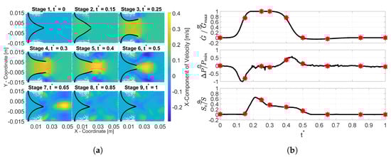
Figure 2.
(a) Each stage represents the results of different stages of the FSI simulation using m/s, s, and MPa. (b) This figure indicates the information (red marks) of the previous nine stages measured for , P, and Sv as a function of . The maximum values obtained are = 0.1446 × m/s, = 163.697 Pa, and S = 0.03 m.
- Stage 1. Initial motionless stage with zero-flow conditions.
- Stage 2. Once flow rate starts to increase from Stage 1 to 2, the leaflets are forced to open as a consequence of a negative pressure difference ().
- Stage 3. The flow rate and Sv reach their maximum values.
- Stage 4. The pressure difference is relatively zero, allowing the leaflets to remain opened.
- Stage 5. The flow rate starts to decrease.
- Stage 6. The increment on the pressure difference () causes a reduction in Sv.
- Stage 7. Leaflet closure only occurs when there is no significant downstream flow rate, producing a pressure difference that is slightly positive.
- Stages 8–9. The last stages show that once there is no flow conditions, the pressure difference and opening area values become zero. This condition does not necessarily mean that the leaflets remain static. Once they are fully closed, they begin to oscillate until the forward stage begins once again.
The design of the input curve avoids a back-flow behavior in the leaflets; consequently, this curve was designed to only provide cases with correct functionality. Despite the slight differences produced by the 2D simplification, previous results on the FSI simulation of leaflets [15] showed a qualitative agreement with the aforementioned experimental case [42]. Finally, in order to observe the behavior of the leaflets under different conditions, a parametric study was carried out. The variations consisted of changing the elastic modulus (E) in the solid domain and the period T of the input signal in the fluid domain. The proposal was to have data of 45 different combinations, retrieved from five variations in E and nine variations in T. All combinations shared the same values of , , , , d, and l and possessed almost the same volume V. The variations for E were chosen considering three different elastic conditions [46]. The first one is for situations where the leaflet material is particularly hard, with . The second considers the opposite, when the leaflet material is extremely soft, resulting in . The last condition considers an intermediate elastic behavior, leading to . From a previos work [42], we considered an initial MPa, two smaller values MPa and MPa, and two larger values MPa and MPa, in order to represent the three aforementioned conditions. More information regarding the mesh-size selection for both the fluid and solid domains, as well as a structural analysis for the leaflet model to obtain the initial conditions for the FSI simulations can be found in the Supplementary Material.
Regarding the variations in T, we initially tested one of the experimental periods proposed where s. Additionally, two more values were chosen from here: s and s. Finally, in order to have nine variations, intermediate values were selected. With these forty-five combinations, we conducted their respective FSI simulations, and the results showed the same behavior as the curves presented in Figure 2. The frequencies, and the corresponding periods, selected for this study are presented in Table 2.
Table 2.
Velocities used for the parametric study.
3. System Identification Method
The main contribution of this paper is to present a complementary method that can help researchers obtain results as accurate as possible as if they were doing an FSI simulation. It has to be considered that the previous simulations are required to obtain the coefficients needed to estimate a specific output parameter. Once the model has been identified, the advantages of this method lie in skipping the many steps required to configure the simulation, namely geometry, boundary conditions, mesh quality, and topology, and mainly to overcome the high computational cost required to accomplish short simulation times and still obtain accurate results.
In general, these systems allow generating a model from the system input/output information. The model selected for these cases is an ARX, which constructs polynomial functions based on a set of coefficients according to the system order n.
ARX Model
The goal of this model is to obtain the vector, which contains the parameters (coefficients) that represent the relation between the input and output of the system.
Hence, the process to calculate the optimal parameter vector can apply the hereditary identification principle by using the experimental expectation [47] instead of the mathematical one [48]. This principle keeps the criterion minimization task quadratic; as a result, it avoids the use of non-linear optimization techniques, such as the gradient-based or Gauss–Newton techniques to derivate and reduce the order of the coefficients. For this case, the distance (the difference) among the estimated trajectories (behavior of the signal after every iteration) is minimized. Hence, we could present:
as the general form to obtain the coefficients , as our main input/output signal using the experimental expectation over , and . Now, in the case of the ARX model, we considered as the output, as the exogenous input, and as the optimal past estimator of the behavior at instant t for data over , and it is calculated as follows:
Then, the regression vector that contains the coefficients to describe the behavior of the system is defined by:
Then, the parameter estimation is done by hereditary computation; therefore, it is required to know the experimental autocorrelation matrix of and the inter-correlation vector of and . Hence, to compute the system parameters at instant t, it is necessary to keep in memory all the past estimations . Therefore, if we were not using hereditary computation, the complexity and computational cost would be higher. The general algorithm used to estimate the vector is:
- Initialization. As data before are unknown, the projection over it is zero (division by a covariance a priori infinite). It is then possible to think of it as zero:
- At instant , we already have data from the previous optimized estimations.
- At instant t, new data are available in order to update the experimental auto-correlation matrix and the inter-correlation vector:
- The coefficient parameter vector at instant t is defined as , and it is obtained by inverting the autocorrelation matrix:
- Hereditary part: With the obtained parameters, by using Equation (6), it is then possible to compute the new estimation based on the previous estimation , which was computed at the preceding stage by employing the model .
- Return to Step 2.
The algorithm describes the process to train only one signal and simulate one output. Hence, in order to obtain each set of coefficients for all forty-five combinations, Figure 3 describes the general process. In this case, the input signal in Figure 3a is equivalent to the input used for the elastic modulus E and time T of the aforementioned ranges of the previous section. With this, we obtained two different outputs (Sv or P) per input from the simulations. The ARX model proposed is a single-input single-output system; hence, each of the forty-five combinations has two ARX models, one per output.
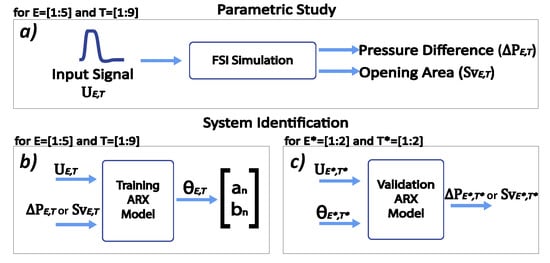
Figure 3.
(a) The parametric study is summarized as a for loop of five variations in E and nine in T. (b) The system identification process uses the input/outputs signals to obtain forty-five vectors. (c) The validation process simulates the output from new input signals for and representing the elastic modulus and periods that were not initially considered in the parametric study.
Secondly, Figure 3b shows the identification part (training), which uses the data obtained in Step (a) to calculate the vector for all combinations. During the estimation, the parameter vector is updated after every iteration and uses the information from previous estimations to reduce the error between the original output and the estimated one. Then, for the combination , the input is equivalent to the exogenous input and or is equivalent to of Equation (6), respectively. Finally, in Figure 3c, the validation part simulates both outputs for a new set of conditions—different from the 45 proposed—by only employing these new input signals and a new set of coefficients, which is calculated by doing a bilinear interpolation with the previous vectors.
4. ARX Model Results
In order to evaluate the quality of the algorithm addressed in this work, we used a multiple correlation coefficient R. This percentage indicates how well explains [48]:
After the training part, we end up having forty-five vectors per output, containing the coefficients’ information. In order to construct the transfer functions, these coefficients follow the next expression (presented in Fourier transform structure) defined in [48].
where is the set of coefficients for the numerator and is the set of coefficients for the denominator. Each output has its own model: for Sv, we employed and ; whereas for P, we used and to represent their respective coefficients. The models have a system order and for the and of the denominator and and for the and of the numerator of each equation. These equations were tested for , and we found the best goodness of fit in P when and ; whereas for Sv, we obtained the best results when and . Hence, according to Equation (13), we have the next structure for the transfer functions of each output using the hereditary ARX computation:
The coefficients found during the identification part for all the elastic moduli proposed are presented as field maps in Figure 4a,b for P and Sv, respectively. In both outputs, we observe that the zone around MPa and s presents the highest or the lowest values, depending on the particular behavior of each coefficient. In the case of P, we see a change close to a local extrema ( MPa and s) for the coefficients, whereas for the , we appreciate this change in the area close to MPa and s. On the other hand, the coefficients for Sv seem to have a constant behavior in all and coefficients surrounding the zone of MPa and s. As mentioned before, the quality of the algorithm was measured using the multiple correlation function R; for that, R values of all combinations are shown in Table 3 (for more details of the entire set of reconstructed signals and the coefficients obtained for the SI model, see the Supplementary Material). In Figure 5a, the curves correspond to the reconstruction of P following the structure of Equation (14), and by comparing them with the experimental curves, their behavior follows the same trend. Conversely, Figure 5b shows that Sv is less accurate, since only the opening and closing moments were recovered; the reconstruction follows Equation (15).
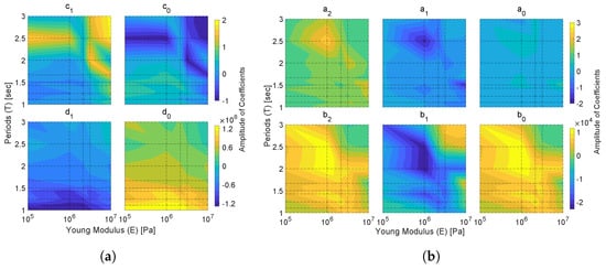
Figure 4.
Coefficient fields obtained from the trained model for all the cases in the parametric study. The dotted lines indicate the nine periods T and the five elastic moduli E. In (a), we have the maps for the P coefficients and, in (b), the coefficients. According to Equations (14) and (15), the values for in P and in are always one.
Table 3.
R values obtained by the AutoRegressive with eXogenous (ARX) input model for both outputs.
Regarding the computational time, the training process for each period took 13 s approximately; hence, obtaining the results of the nine periods for both outputs, for one elastic modulus, took less than 4 min to finish the process. Considering this time, our ARX model calculated all 45 vectors for the training part of both outputs in about 20 min. Thereby, the execution time using the ARX model represents only 0.0465% of the total time (716.5 h) consumed by doing the forty-five FSI simulations of the parametric study. This means that once our model is trained, we can obtain estimations to complement further cases with it instead of doing more FSI simulations, which would require more computational time.
4.1. ARX Model Validation
One of the main goals of using an ARX model for this purpose is to have the possibility to use the parameter vectors found in the training part for estimating/simulating external conditions to the ones employed in the parametric study and verify the quality of our model without spending more time on FSI simulations. The simulation parameters considered for these changes are the same as the ones in the parametric study except for E and T. These parameters now consider the following options: [1.5, 15] MPa and [0.90, 1.20]s. The selected ranges are close to the elastic conditions proposed in Section 2.1, and this allowed us to verify the behavior of our model in four different situations:
- (1)
- E = 1.5 MPa, T = 0.9 s: the elastic modulus lies inside, and the period is outside the training dataset.
- (2)
- E = 1.5 MPa, T = 1.2 s: both conditions are located inside the training dataset.
- (3)
- E = 15 MPa, T = 0.9 s: both conditions lie outside the training dataset.
- (4)
- E = 15 MPa, T = 1.2 s: the elastic modulus is outside the training dataset, whereas the period is located inside it.
The validation process forms the transfer functions of the aforementioned desired values by using a bilinear interpolation with the coefficients found in Figure 4. Finally, Table 4 presents the interpolated values for these new cases.
Table 4.
Coefficients calculated for the validation process.

Figure 5.
Signals reconstructed using the ARX model for MPa during the training process. In (a), the pressure difference (P) and, in (b), the normalized opening area (). The average accuracy obtained for reconstructing the nine periods was and for P and respectively. The average goodness of fit of the five is listed in Table 5.
Table 5.
Average goodness of fit obtained for the training and validation processes.
Figure 5.
Signals reconstructed using the ARX model for MPa during the training process. In (a), the pressure difference (P) and, in (b), the normalized opening area (). The average accuracy obtained for reconstructing the nine periods was and for P and respectively. The average goodness of fit of the five is listed in Table 5.

In order to compare the signals obtained by our ARX model, we previously conducted the FSI simulations of these new conditions used for validation. The results seen in Figure 6 show that some simulations were not able to finish the calculation process; this was because they were unable to find equilibrium or convergence. For these reasons, estimation of the outputs was merely conducted until the moment before the simulation stopped. The accuracy of the validation results is shown Table 5, where the average value of accuracy was and for Sv and P, respectively.
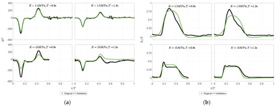
Figure 6.
Validation results obtained using the coefficients maps to interpolate and extrapolate the new cases. In (a) we have results for the pressure difference cases and in (b) the reconstructed signals for opening area.
One limitation of this method is that it only works for stationary signals; hence, when dealing with transitory behaviors, it was not able to follow the trend expected efficiently. For example, in the opening area of Figure 6, we can see at the beginning of the forward stage (tf) how the leaflets began to open up to the highest position due to an inertial momentum before it went back to the value where it got stabilized by the flow. On the contrary, the pressure difference output was better estimated by our model because it did not contain a transitory behavior.
This validation process showed that our model could be a promising support for the FSI simulations when dealing with different situations in a faster and still accurate way. Besides, it could eliminate the necessity of conducting several simulations before we can get a vast amount of information by making small changes in the input signal and wait for very long times to see how these new conditions behave. We remark that our model follows trends, and it may require complementary techniques such as non-linear models to fully estimate the outputs.
4.2. Test for Gaussianity and Linearity
According to the results, our model proved to have better performance when dealing with the pressure difference than with the opening area. Hence, as a final step, we analyzed the prediction error vector obtained in Sv to verify its distribution (Gaussian or non-Gaussian) and its possible non-linear behavior in some sections. The test proposed by Hinich [49] assumes two different hypotheses: the first one is to verify if the process is Gaussian distributed or not; then, if the first hypothesis is accepted, the second one consists of verifying whether the process is linear or not. Therefore, for Gaussianity, we have a Probability of False Alarm (PFA) parameter that indicates the probability that our data have a non-zero bispectrum. Hence:
Hypothesis 1:
If ; the process is non-Gaussian, i.e., non-zero bispectrum.
Hypothesis 2:
If ; the process is Gaussian, i.e., zero bispectrum.
Then, if Hypothesis 1 is true, we can test to verify if it contains linear or non-linear behavior. Since this test assumes a non-zero bispectrum, it should only be considered if and only if obtained a . Thus, is the estimated and is the theoretical interquartile range of a chi-squared distribution:
Hypothesis 3:
If or , the process is non-linear.
Hypothesis 4:
If , the process is linear.
Under these assumptions, we use the High Order Spectral Analysis (HOSA) toolbox for MATLAB to conduct the test. Results in Table 6 show that all our vectors are non-Gaussian distributions and contain non-linear processes within them. Conclusively, for providing a more accurate analysis, future experiments should include a model that considers the estimation of these potential non-linear processes as well. For more details, see [49,50].
Table 6.
Results of Gaussianity and the linearity test for the Sv output.
5. Discussion
The main contribution of this paper is to provide a complementary method to avoid continuous repetitions of FSI simulations to know the behavior of an idealized and simplified academic problem, which studies two leaflets inside a channel and its interaction with a surrounding flow. We propose the use of a SI model to reduce the excessive computational time required to perform many repetitions of the same design under different flow conditions. The 2D leaflets’ structure simplification is taken from the experimental case found in [42], and it considers as outputs the opening area and pressure difference of the leaflets under a pulsatile flow. For our case, the input signal is only transmitted along two directions (x and y planes) and not in three, as the experimental setup. Besides, the experimental data are averaged across all cycles to produce a single representative cycle, reducing all possible measurement noise. On the contrary, FSI simulations are merely carried out for a single cycle; hence, noise reduction by averaging the signal was not possible.
The SI method proposed is an ARX model that uses the information retrieved by the FSI simulations of a parametric study to obtain coefficients for the transfer functions that represent the specific outputs. With the parameter vectors obtained, we create coefficient maps to observe the behavior of each one for all the cases studied. Using these coefficient fields, we employ interpolations to obtain the values for the desired conditions in the validation process. These validation parameters are selected to have two cases within the dataset and two outside the dataset. The coefficients obtained from this step are used to create the transfer functions that estimate the trend of the output without the need for conducting continuous FSI simulations. Finally, the estimation performed for the validation process proves that the closer the parameters are to the dataset, the better the agreement of the simulated signal to be compared with the FSI results. On the other side, the cases that are outside or slightly far from the conditions of the dataset obtain a less accurate estimation, which however, still follows the trend of the signal.
6. Conclusions
A first approach to simulate the output of a simple leaflet model by employing a system identification method is presented. This model uses the information from previous FSI simulations to be trained and obtain a coefficient vector, which is later used in addition to an input signal to simulate the opening area and pressure difference outputs. Despite the fact that FSI simulations are a more complete tool to study this phenomena, our model could provide complementary help to obtain results in a faster way once it is trained. This method provided accurate tracking of the trends of those outputs with no transitory behaviors, but it does not sufficiently simulate the behavior of outputs that contain transitory ones. In this way, if we consider data retrieved from FSI simulations of more realistic 3D geometries with real patient data, we could also train our ARX model to get the necessary coefficients in order to simulate the output of such scenarios. This could lead to using this supplementary method in situations where faster analysis is required in hospitals without having to wait for longer periods, as it would be by only using FSI simulations. Furthermore, speaking of clinical or practical applications, with the implementation of a moving average (ARMAX) term, which minimizes the error, we could propose a prognostic health management process. By using data from real patients, we could make a classifier that, according to the coefficients obtained in the ARMAX model, we could infer the current health status of a person. The main difference with the ARX model is that ARMAX also considers the original output for the prediction error reduction and the adjustment of the coefficients.
The parametric study presented in this paper considers FSI simulations with five variations in the elastic modulus E and nine variations in the period T, and it is used to train the model under a small set of conditions. Additionally, the ARX model trained takes approximately 20 minutes to finish all the coefficients calculation, which represents only 0.0465% of the time used by FSI simulations. Furthermore, the data generated by the FSI simulations need a post-processing (another five minutes approximately) before we can use them in the ARX model; giving a total time of less than 25 minutes to finish the training and validation processes of all data. The validation process is conducted by using interpolation to obtain the transfer functions that represent the conditions that are not initially considered for the parametric study. The proposed ARX method is able to follow the trend with 90.14% and 92.27% of accuracy respectively for Sv and P. The identification stage considers 45 combinations per output; whereas, for the validation part, we obtain an average accuracy of 93.31% and 83.08% for Sv and P for four combinations per output. The validation results show that our model is able to follow the behavior of both outputs in a better way when the conditions are inside or close to the boundaries of our training dataset conditions. Finally, a linearity test proves that the prediction error of these signals contains non-linear behavior; hence, future work includes further study of these processes through a non-linear system identification model.
Supplementary Materials
The following are available online at https://www.mdpi.com/2076-3417/10/22/8228/s1, Table S1. Results obtained for the solid mesh size test, Figure S1: Validation test for the solid mesh selection, Figure S2. Meshes distribution -sections- within the layout., Figure S3. Validation test for the fluid mesh selection, Figure S4. Displacement observed in the top leaflet after T= 3s, Figure S5. The behavior of the leaflet indicates oscillation moments increased as soon as the elastic modulus did, whereas the magnitude of these reduces with a higher E value, Table S3. Displacement of each E under different forces applied, Figure S6. Reconstruction of the signals using the ARX model for E = 0.1 MPa. In (a) we have the opening area and in (b) the pressure difference, Table S4. Coefficients obtained for (a) Sv and (b) DP corresponding to E = 0.1 MPa., Figure S7. Reconstruction of the signals using the ARX model for E = 1 MPa. In (a) we have the opening area and in (b) the pressure difference, Table S5. Coefficients obtained for (a) Sv and (b) DP corresponding to E = 1 MPa., Figure S8. Reconstruction of the signals using the ARX model for E = 3.16 MPa. In (a) we have the opening area and in (b) the pressure difference, Table S6. Coefficients obtained for (a) Sv and (b) DP corresponding to E = 3.16 MPa., Figure S9. Reconstruction of the signals using the ARX model for E = 10 MPa. In (a) we have the opening area and in (b) the pressure difference, Table S7. Coefficients obtained for (a) Sv and (b) DP corresponding to E = 10 MPa.
Author Contributions
C.D.-H. was responsible of the investigation, configuration, and testing for all the material presented and also the writing of this article. G.E. and R.L.-A. supervised all processes and experimentation in this work and also contributed with corrections, guidance, writing, reviewing, and editing of this document. All authors read and agreed to the published version of the manuscript.
Funding
This research received no external funding.
Conflicts of Interest
The authors declare no conflict of interest.
References
- Ljung, L. Perspectives on system identification. Annu. Rev. Control 2010, 34, 1–12. [Google Scholar] [CrossRef]
- Haddouche, R.; Chetate, B.; Boumedine, M.S. Neural network ARX model for gas conditioning tower. Int. J. Model. Simul. 2019, 39, 166–177. [Google Scholar] [CrossRef]
- Sarwar, R.; Cho, H.; Cox, S.J.; Mago, P.J.; Luck, R. Field validation study of a time and temperature indexed autoregressive with exogenous (ARX) model for building thermal load prediction. Energy 2017, 119, 483–496. [Google Scholar] [CrossRef]
- Huang, K.Y.; Jane, C.J. A hybrid model for stock market forecasting and portfolio selection based on ARX, grey system and RS theories. Expert Syst. Appl. 2009, 36, 5387–5392. [Google Scholar] [CrossRef]
- Okuda, H.; Ikami, N.; Suzuki, T.; Tazaki, Y.; Takeda, K. Modeling and analysis of driving behavior based on a probability-weighted ARX model. IEEE Trans. Intell. Transp. Syst. 2012, 14, 98–112. [Google Scholar] [CrossRef]
- Zeng, X.; Wang, J. A stochastic driver pedal behavior model incorporating road information. IEEE Trans. Hum. Mach. Syst. 2017, 47, 614–624. [Google Scholar] [CrossRef]
- Yang, M.; Makis, V. ARX model-based gearbox fault detection and localization under varying load conditions. J. Sound Vib. 2010, 329, 5209–5221. [Google Scholar] [CrossRef]
- Nguyen, Q.C.; Vu, V.H.; Thomas, M. ARX Model for Experimental Vibration Analysis of Grinding Process by Flexible Manipulator. In Proceedings of the Surveillance, Vishno and AVE conferences, INSA-Lyon, Universite de Lyon, Lyon, France, 8–10 July 2019. [Google Scholar]
- Qin, Y.; Peng, H.; Ruan, W.; Wu, J.; Gao, J. A modeling and control approach to magnetic levitation system based on state-dependent ARX model. J. Process. Control 2014, 24, 93–112. [Google Scholar] [CrossRef]
- Tian, X.; Peng, H.; Zeng, X.; Zhou, F.; Xu, W.; Peng, X. A modelling and predictive control approach to linear two-stage inverted pendulum based on RBF-ARX model. Int. J. Control 2019, 1–19. [Google Scholar] [CrossRef]
- Tran, N.T.; Khan, A.; Choi, W. State of charge and state of health estimation of AGM VRLA batteries by employing a dual extended kalman filter and an ARX model for online parameter estimation. Energies 2017, 10, 137. [Google Scholar] [CrossRef]
- Romero-Ugalde, H.M.; Garnotel, M.; Doron, M.; Jallon, P.; Charpentier, G.; Franc, S.; Huneker, E.; Simon, C.; Bonnet, S. ARX model for interstitial glucose prediction during and after physical activities. Control Eng. Pract. 2019, 90, 321–330. [Google Scholar] [CrossRef]
- Fetics, B.; Nevo, E.; Chen, C.H.; Kass, D.A. Parametric model derivation of transfer function for noninvasive estimation of aortic pressure by radial tonometry. IEEE Trans. Biomed. Eng. 1999, 46, 698–706. [Google Scholar] [CrossRef] [PubMed]
- Liu, Y.; Birch, A.; Allen, R. Dynamic cerebral autoregulation assessment using an ARX model: Comparative study using step response and phase shift analysis. Med. Eng. Phys. 2003, 25, 647–653. [Google Scholar] [CrossRef]
- Duran-Hernandez, C.; Perez-Santiago, R.; Etcheverry, G.; Ledesma-Alonso, R. Modeling of a Simplified 2D Cardiac Valve by Means of System Identification. In Proceedings of the MCPR: Pattern Recognition, Querétaro, Mexico, 26–29 June 2019; pp. 371–380. [Google Scholar]
- Horsten, J.B.A.M. On the Analysis of Moving Heart Valves: A Numerical Fluid-Structure Interaction Model. Ph.D. Thesis, Technische Universiteit Eindhoven, Eindhoven, The Netherlands, 1990. [Google Scholar]
- Chandra, S.; Rajamannan, N.M.; Sucosky, P. Computational assessment of bicuspid aortic valve wall-shear stress: Implications for calcific aortic valve disease. Biomech. Model. Mechanobiol. 2012, 11, 1085–1096. [Google Scholar] [CrossRef] [PubMed]
- Peskin, C.S. Flow patterns around heart valves: A numerical method. J. Comput. Phys. 1972, 10, 252–271. [Google Scholar] [CrossRef]
- Gao, H.; Feng, L.; Qi, N.; Berry, C.; Griffith, B.E.; Luo, X. A coupled mitral valve—Left ventricle model with fluid–structure interaction. Med. Eng. Phys. 2017, 47, 128–136. [Google Scholar] [CrossRef]
- Sigüenza, J.; Pott, D.; Mendez, S.; Sonntag, S.J.; Kaufmann, T.A.; Steinseifer, U.; Nicoud, F. Fluid-structure interaction of a pulsatile flow with an aortic valve model: A combined experimental and numerical study. Int. J. Numer. Methods Biomed. Eng. 2018, 34, e2945. [Google Scholar] [CrossRef]
- Mao, W.; Li, K.; Sun, W. Fluid-Structure interaction study of transcatheter aortic valve dynamics using smoothed particle hydrodynamics. Cardiovasc. Eng. Technol. 2016, 7, 374–388. [Google Scholar] [CrossRef]
- Stijnen, J.; De Hart, J.; Bovendeerd, P.; Van de Vosse, F. Evaluation of a fictitious domain method for predicting dynamic response of mechanical heart valves. J. Fluids Struct. 2004, 19, 835–850. [Google Scholar] [CrossRef]
- De Hart, J.; Peters, G.W.; Schreurs, P.J.; Baaijens, F.P. A two-dimensional fluid-structure interaction model of the aortic value. J. Biomech. 2000, 33, 1079–1088. [Google Scholar] [CrossRef]
- De Hart, J.; Peters, G.; Schreurs, P.; Baaijens, F. A three-dimensional computational analysis of fluid–structure interaction in the aortic valve. J. Biomech. 2003, 36, 103–112. [Google Scholar] [CrossRef]
- Kamensky, D.; Hsu, M.C.; Schillinger, D.; Evans, J.A.; Aggarwal, A.; Bazilevs, Y.; Sacks, M.S.; Hughes, T.J. An immersogeometric variational framework for fluid–structure interaction: Application to bioprosthetic heart valves. Comput. Methods Appl. Mech. Eng. 2015, 284, 1005–1053. [Google Scholar] [CrossRef] [PubMed]
- Xu, F.; Morganti, S.; Zakerzadeh, R.; Kamensky, D.; Auricchio, F.; Reali, A.; Hughes, T.J.; Sacks, M.S.; Hsu, M.C. A framework for designing patient-specific bioprosthetic heart valves using immersogeometric fluid-structure interaction analysis. Int. J. Numer. Methods Biomed. Eng. 2018, 34, e2938. [Google Scholar] [CrossRef] [PubMed]
- Mao, W.; Caballero, A.; McKay, R.; Primiano, C.; Sun, W. Fully-coupled fluid-structure interaction simulation of the aortic and mitral valves in a realistic 3D left ventricle model. PLoS ONE 2017, 12, e0184729. [Google Scholar] [CrossRef] [PubMed]
- Singh-Gryzbon, S.; Sadri, V.; Toma, M.; Pierce, E.L.; Wei, Z.A.; Yoganathan, A.P. Development of a Computational Method for Simulating Tricuspid Valve Dynamics. Ann. Biomed. Eng. 2019, 47, 1422–1434. [Google Scholar] [CrossRef]
- Mohammed, A.M.; Ariane, M.; Alexiadis, A. Using Discrete Multiphysics Modelling to Assess the Effect of Calcification on Hemodynamic and Mechanical Deformation of Aortic Valve. ChemEngineering 2020, 4, 48. [Google Scholar] [CrossRef]
- Caballero, A.; Mao, W.; McKay, R.; Sun, W. Transapical mitral valve repair with neochordae implantation: FSI analysis of neochordae number and complexity of leaflet prolapse. Int. J. Numer. Methods Biomed. Eng. 2020, 36, e3297. [Google Scholar] [CrossRef]
- Caballero, A.; McKay, R.; Sun, W. Computer simulations of transapical mitral valve repair with neochordae implantation: Clinical implications. JTCVS Open 2020, 3, 27–44. [Google Scholar] [CrossRef]
- Lee, J.H.; Rygg, A.D.; Kolahdouz, E.M.; Rossi, S.; Retta, S.M.; Duraiswamy, N.; Scotten, L.N.; Craven, B.A.; Griffith, B.E. Fluid-Structure Interaction Models of Bioprosthetic Heart Valve Dynamics in an Experimental Pulse Duplicator. Ann. Biomed. Eng. 2020, 48, 1–16. [Google Scholar] [CrossRef]
- Xu, F.; Johnson, E.L.; Wang, C.; Jafari, A.; Yang, C.H.; Sacks, M.S.; Krishnamurthy, A.; Hsu, M.C. Computational investigation of left ventricular hemodynamics following bioprosthetic aortic and mitral valve replacement. Mech. Res. Commun. 2020, 2020, 103604. [Google Scholar] [CrossRef]
- Toma, M.; Einstein, D.R.; Kohli, K.; Caroll, S.L.; Bloodworth, C.H.; Cochran, R.P.; Kunzelman, K.S.; Yoganathan, A.P. Effect of Edge-to-Edge Mitral Valve Repair on Chordal Strain: Fluid-Structure Interaction Simulations. Biology 2020, 9, 173. [Google Scholar] [CrossRef] [PubMed]
- Toma, M.; Einstein, D.R.; Bloodworth, C.H.; Kohli, K.; Cochran, R.P.; Kunzelman, K.S.; Yoganathan, A.P. Fluid-Structure Interaction Analysis of Subject-Specific Mitral Valve Regurgitation Treatment with an Intra-Valvular Spacer. Prosthesis 2020, 2, 7. [Google Scholar] [CrossRef]
- Peña Pérez, N. Windkessel Modeling of the Human Arterial System. Bachelor’s Thesis, University Carlos III of Madrid, Madrid, Spain, 13 July 2016. [Google Scholar]
- Westerhof, N.; Lankhaar, J.W.; Westerhof, B.E. The arterial windkessel. Med. Biol. Eng. Comput. 2009, 47, 131–141. [Google Scholar] [CrossRef] [PubMed]
- Xu, P.; Liu, X.; Zhang, H.; Ghista, D.; Zhang, D.; Shi, C.; Huang, W. Assessment of boundary conditions for CFD simulation in human carotid artery. Biomech. Model. Mechanobiol. 2018, 17, 1581–1597. [Google Scholar] [CrossRef]
- Pant, S.; Corsini, C.; Baker, C.; Hsia, T.Y.; Pennati, G.; Vignon-Clementel, I.E.; Modeling of Congenital Hearts Alliance (MOCHA) Investigators. Data assimilation and modelling of patient-specific single-ventricle physiology with and without valve regurgitation. J. Biomech. 2016, 49, 2162–2173. [Google Scholar] [CrossRef]
- Huang, H.; Shu, Z.; Song, B.; Ji, L.; Zhu, N. Modeling left ventricular dynamics using a switched system approach based on a modified atrioventricular piston unit. Med. Eng. Phys. 2019, 63, 42–49. [Google Scholar] [CrossRef]
- Pironet, A.; Dauby, P.C.; Chase, J.G.; Docherty, P.D.; Revie, J.A.; Desaive, T. Structural identifiability analysis of a cardiovascular system model. Med. Eng. Phys. 2016, 38, 433–441. [Google Scholar] [CrossRef]
- Ledesma-Alonso, R.; Guzmán, J.; Zenit, R. Experimental study of a model valve with flexible leaflets in a pulsatile flow. J. Fluid Mech. 2014, 739, 338–362. [Google Scholar] [CrossRef]
- Duran-Hernandez, C.; Ledesma-Alonso, R.; Etcheverry, G.; Perez-Santiago, R. Aerodynamic Coefficient Calculation of a Sphere Using Incompressible Computational Fluid Dynamics Method. In Technology, Science, and Culture: A Global Vision; IntechOpen: Puebla, Mexico, 2018; pp. 105–112. [Google Scholar]
- Sundaram, G.B.K.; Balakrishnan, K.R.; Kumar, R.K. Aortic valve dynamics using a fluid structure interaction model–The physiology of opening and closing. J. Biomech. 2015, 48, 1737–1744. [Google Scholar] [CrossRef]
- Kunzelman, K.; Einstein, D.R.; Cochran, R. Fluid–structure interaction models of the mitral valve: Function in normal and pathological states. Philos. Trans. R. Soc. Biol. Sci. 2007, 362, 1393–1406. [Google Scholar] [CrossRef]
- Amindari, A.; Saltik, L.; Kirkkopru, K.; Yacoub, M.; Yalcin, H.C. Assessment of calcified aortic valve leaflet deformations and blood flow dynamics using fluid-structure interaction modeling. Inform. Med. Unlocked 2017, 9, 191–199. [Google Scholar] [CrossRef]
- Monin, A.; Salut, G. ARMA lattice identification: A new hereditary algorithm. IEEE Trans. Signal Process. 1996, 44, 360–370. [Google Scholar] [CrossRef]
- Ljung, L. System Identification: Theory for the User; Prentice-Hall: Englewood Cliffs, NJ, USA, 1987. [Google Scholar]
- Hinich, M.J. Testing for Gaussianity and linearity of a stationary time series. J. Time Ser. Anal. 1982, 3, 169–176. [Google Scholar] [CrossRef]
- Swami, A.; Mendel, J.M.; Nikias, C.L. Higher-Order Spectral Analysis Toolbox; The Mathworks Inc.: Natick, MA, USA, 1995. [Google Scholar]


Publisher’s Note: MDPI stays neutral with regard to jurisdictional claims in published maps and institutional affiliations. |
© 2020 by the authors. Licensee MDPI, Basel, Switzerland. This article is an open access article distributed under the terms and conditions of the Creative Commons Attribution (CC BY) license (http://creativecommons.org/licenses/by/4.0/).