Piezoelectric Energy Harvesting Prediction and Efficient Management for Industrial Wireless Sensor

Featured Application

The work proposes A New Method to Design Autonomous Wireless Sensor to support Industrial Applications of the Internet of Things.

Abstract

The vibrations, due to their abundance in most industrial processes, constitute an attractive solution for the power supply of Industrial Wireless Sensor (IWS). However, the amount of energy that can be harvested presents numerous fluctuations due to the engines’ different operating modes (overload, full load, or even operation without charge). Most designs do not incorporate this fluctuation in the definition of the specifications of the autonomous IWS. This paper then presents a design method to ensure the node’s energy autonomy while maximizing its Quality of Service (QoS). To precisely define the specifications of the IWS, vibration measurements were carried out at its location for one month. The recorded data was used to propose a new Predictor of the Harvestable Energy from Vibrations (PHEV). A comparative evaluation of the proposed PHEV performances with a state-of-the-art predictor is carried out. The results obtained show that the PHEV makes it possible to minimize the Root Mean Square Error (RMSE) from $28.63 \mathrm{mW}$ to $19.52 \mathrm{mW}$. A model of energy dissipation in IWS, considering the Internet of Things’ requirements, was established. The model is based on Long-Range (LoRa)/Long-Range Communication Wide Area Network (LoRaWan). The amount of data transmitted is then maximized according to the expected energy harvest rate by setting up a Maximization Data Size Protocol (MDSP). The proposed method makes it possible to ensure an acceptable QoS without resorting to reconfigurable circuits, which are sometimes bulky for miniature devices such as the IWS.

1. Introduction

Numerous studies have shown that benefits such as increased productivity, security, efficiency, and even lower costs are due to the automation of most industrial processes [1]. Moreover, these are the objectives of Industry 4.0, which aims to transform all the processes of a factory into an interconnected global system. At the base of automated systems, there are sensors whose function is to transmit information on the system’s state at regular time intervals. More specifically, in the industrial environment, the sensors are used in automation systems [2], operation controls, system monitoring (humidity, temperature, fire alarm, dust index, toxic gas, and pollution) [2,3,4], and motion control [5].

The used sensors in the industrial process can be wired or wireless; when these sensors are wireless, they are referred to as Industrial Wireless Sensors (IWSs). When the process to be monitored requires several sensors, the numerous wired connections can be troublesome for the process. For this reason, IWSs have experienced enthusiastic support because of their small dimensions, their ease of deployment, their flexibility, and their low cost [6]. These numerous advantages are, unfortunately, accompanied by the issue of their energy supply. Since IWSs are battery-powered, recharging or replacement operations are very costly because they require a cessation of production. The solutions for harvesting ambient energy, which consists of transforming an energy source located in the sensor’s immediate environment into electrical energy for its supply, are then considered.

Many energy harvesting techniques are offered; the difference is likely the primary source used (sun, vibrations, radiofrequency waves, heat, internal light, etc.). Sources such as the sun provide significant amounts of energy that can even be fed back into the national grid; however, the sunshine level is deficient in confined spaces. Recently, radio waves have also been used to recharge IWS batteries [7]. Unfortunately, the amount of ambient radiofrequency energy that can be harvested is limited due to potential health concerns [8]. Concerning the heat, previous work has shown that conversion efficiencies are extremely low [9]. Thus, for industrial applications, vibrations are the most considered energy source to power the IWS [10].

1.1. Literature Overview and Main Problematic

Three transduction mechanisms, namely electrostatic, electromagnetic, and piezoelectric, are considered to convert vibrations into electrical energy. Piezoelectric transducers (PTs) are the most considered because of their strong electromechanical coupling and the ease of integrating them into the desired applications [11]. As most vibration applications in industrial processes are low frequency, PT architecture is of the cantilever type [12]. The main problem linked to cantilever PTs’ design is their narrow bandwidth, resulting in low conversion efficiency when the main vibration frequency fluctuates. The main techniques for increasing the PT’s efficiency include non-linearity and de circuit management [13].

The research carried out in non-linear modules offers solutions to amplify the voltage and the maximum energy transferred to the load. The most used non-linear techniques are the Synchronized Switch Harvesting on Inductor (SSHI) [14], the Synchronized Switch Harvesting on Capacitor (SSHC) [15], and the Synchronous Electric Charge Extraction (SECE) [16]. These techniques are derived from the Synchronized Switch Damping on Inductor (SSDI) proposed in [17] to cushion vibrations in mechanical systems. In the SSDI technique, by connecting to the piezoelectric material, a passive electrical load, it can transfer some of the mechanical energy in an electrical form, leading to mechanical damping [18]; therefore, maximizing the recovered electrical power. Practically, a switch is used to insert into the PT’s circuit as it passes through its maximum voltage, an impedance that is dual to the PT’s internal impedance; this has caused an increase in the current through the dual impedance. This current decreases by recharging the PT’s impedance to a voltage reverse to its initial voltage, giving rise to a voltage greater than the PT’s maximum initial voltage [19]. For example, using the SSHI technique was possible in [20] to harvest 200% more power than with a standard PT at a frequency of 30 Hz. In [15], using the SSHC technique, it was possible to amplify the harvested power six times compared to the standard PT this at an excitation frequency of 22 Hz. As can be seen, although these solutions help to amplify the level of harvestable power, they are still offered for a fixed excitation of the PT. Unfortunately, in actual use, the vibrations’ fundamental frequency changes according to the engine’s operating speed, which generates the waves. In most industrial processes, the motor at a given moment may find itself at full load or overload and even sometimes at no charge. These different operating regimes will cause a fluctuation in the harvestable energy. The vibrations’ primary frequency changes give rise to the PTs’ low efficiencies in real situations.

Other design methods aim to tune the transducer’s resonant frequency to the main frequency of the vibrations to overcome this limitation. For this, some research suggests broadband or multiband transducers [21,22]. However, designing such kinds of PT is accompanied by an increase in the size of the circuits, which can prove to be cumbersome for miniature components such as IWS.

Another method to make an IWS operational under the harvested energy, without resorting to bulky circuits consists of storing energy until it is enough to allow the node to transmit data. This research field concerns the management of harvestable energy, and this energy harvesting technique is known in the literature as Harvest-Store-Use (HSU) [23]. Very often, the method allows the node to operate perpetually, but this is to the detriment of the Quality of Service (QoS) since it is difficult to predict the frequency of data transmission and the amount of data that the IWS can transmit at a given time. For example, in [19], the vibration data from a mining locomotive are used to design a piezoelectric micro-generator, which incorporates most of the optimizations proposed in the literature, in particular, the non-linear SSHI technique. The designed circuit allowed an IWS to transmit data with 512 bits at less than a kilometer every 7 min. Note that in most IoT applications, events can occur at any time, so it is essential to provide the node with the ability to transmit data at regular time intervals. This work then dealt with the random amount of energy harvested from vibrations to supply IWSs. As mentioned above, this problem is always present in vibrational energy harvesting regardless of the electromechanical used conversion model. This work then proposes designing a predictor of the harvestable energy of vibrations to optimize the potential of the autonomous IWS.

Much work has been proposed in recent years to predict environmental harvestable energy rates for powering wireless sensors [24,25,26]. However, these researches consider solar energy and have been facilitated by the accessibility to weather forecasts commonly provided for different regions. Note that the prediction of harvestable energy is a prerequisite for the efficient management of the harvested energy. In [26], for example, using a 7-day sun database, Kansal et al. have proposed a predictor of harvestable energy. Depending on the harvested power, the management module ensuring the sensor in an Energy-Neutral Operation (ENO) state has been implemented. The ENO state consists of conditioning the sensor to always lower energy expenditure than the harvested energy. Studies on predicting harvestable energy from vibrations have received little consideration, primarily due to a database lack. Secondly, numerous fluctuations appearing in some spectra of vibrations proposed in the literature have reduced researchers’ interest in predicting the level of harvestable energy [12,26]. Thus, in the design method proposed here, it will first be a question of defining a sufficient database of vibrations to establish a model making it possible to quantify the rate of harvestable power. Based on this issue, the main contributions of this paper are further described in the following subsection.

1.2. Motivation and Main Contribution

As mentioned above, this work’s main issue is the fluctuating character (due to the engines’ operating regime that varies depending on its load) of the amount of energy harvestable from vibrations for supplying the IWSs. Thus, this work’s first contribution will then be to design a harvestable energy predictor from an industrial process’s vibrations.

The above literature overview has also highlighted the need to focus not only on the harvestable energy rate but also on the efficient management of this energy. However, most studies are limited to the performance of the PT without defining the IWS stand-alone specifications. For example, in [27], a PT capable of harvesting power of $8.9 \mathrm{mW}$ at $8.3 \mathrm{Hz}$ is proposed; it would then be interesting to define an application (data size, transmission frequency, or transmission range) for this energy level. The architecture of the proposed system in our study is shown in Figure 1 below. The system includes the IWS, which must measure, process, and transmit the data to a collection point called Base Station (BS). A Predictor of the Harvestable Energy from Vibrations (PHEV) is used to predict the amount of energy available in each transmission cycle. Under the basis of the available power and the sensor’s energy requirement, the Power Management Module (PMM) defines the maximum size of the data that can be transmitted to the BS.

To quantify the sensor energy requirement, it is necessary to consider the hardware components of the IWS. The hardware is based on three main parts shown in Figure 1 (the sensor, the microprocessor, and the RF transceiver). The characteristics of some ultra-low consumption components currently marketed are shown in

Table 1. Some IWSs commercial off-the-shelf components and nominal power consumption specifications.

Sensors		Microprocessor		Radio Chip
Components	Power consumption in active mode	Components	Power consumption in active mode	Components	Transmit power consumption
ADXL35 (Accelerometer of Analog Devices)	$1.8 \mathrm{V} @ 0.35 \mathrm{mA}$ [29]	MSP430G2553 of Texas Instrument	$1.8 \mathrm{V} @ 0.23 \mathrm{mA}$ [30]	CC2430 of Texas Instrument	$2 \mathrm{V} @ 27 \mathrm{mA}$ [28]
STLM20 (Temperature sensor of ST)	$2.4 \mathrm{V} @ 0.008 \mathrm{mA}$ [31]	MSP430L092 of Texas Instrument	$0.9 \mathrm{V} @ 0.18 \mathrm{mA}$ [32]	CC2520 of Texas Instrument	$1.8 \mathrm{V} @ 18.5 \mathrm{mA}$ [33]
MPL115A (Pressure sensor of Freescale)	$3.3 \mathrm{V} @ 0.005 \mathrm{mA}$ [34]	ATMega128 of Atmel	$2.7 \mathrm{V} @ 8 \mathrm{mA}$ [35]	SX1211 of Semtech	$2.1 \mathrm{V} @ 25 \mathrm{mA}$ [36]

. From the electrical characteristics taken from the component datasheets, the most significant consumption is due to the data communication with power levels of up to $54 \mathrm{mW}$ if we consider the case of the CC2430 transmitter from Texas Instruments [28]. These consumption levels will be even higher if the sensor’s energy consumption during sleep mode is considered.

The PT must supply the above power levels;

Table 2. Some marketed piezoelectric transducer.

PT	Frequency Range (Hz)	Power	$\mathbf{Size} \left(\mathbf{c}{\mathbf{m}}^3\right)$
Mide volture [37,39]	$50–200$	$9 \mathrm{mW} @ 1 \mathrm{g}$	$3$
Piezo System [40]	$52$	$7.1 \mathrm{mW} @ 2.6 \mathrm{mm} \left(\mathrm{deflexion}\right)$	$3.3$
MicroGen System [41]	$\mathrm{100,120}$ and $600$	$0.85 \mathrm{mW} @ 600 \mathrm{Hz};0.5 \mathrm{g}$	$0.7$
PMG Perpetuum [42]	50 and 60 Hz	$25.5 \mathrm{mW}$	---

carries some PT currently marketed and the power density’s performance. The most popular and increasingly used transducers are those of Mide-Technology [37] because of their high-power density. From the characteristics in Table 2, it appears that the commercially available transducers are useful for a specific predefined frequency band. The power levels supplied are low compared to the energy requirements reported in Table 1. Some research has investigated this issue, and the proposed method is to leave the sensor in sleep mode as long as the stored energy is not sufficient for transmission. For example, in [38], it took 12 h of charging on a 0.33 pF capacitor before the sensor was able to transmit data. In [19], only 512 bits was transmissible every 7 min at less than one kilometer. This poor QoS is because most of the consumption models considered for stand-alone IWSs are based on short-range communication modules like the CC2520 from Texas Instruments. Thus, the solutions proposed so far come to the detriment of the QoS of the IWS, which justifies the need for a new design method, which is the goal of this paper. It is then proposed here to define the specifications of the IWS based on the possibility of predicting the amount of energy harvested during each measurement cycle. The main contributions are to design a predictor of harvestable energy of the surrounding vibrations and the implementation of protocols allowing the IWS to transmit a certain amount of data in each measurement cycle; the different stages of this new design method are described in the next subsection.

1.3. The Method, Assumptions, and Paper Organization

In this work, it is proposed to analyze the vibrations at the location of the IWS before conception. The analysis of fluctuations over a very long-time interval will make it possible to design a predictor of the harvestable energy subsequently. The specifications of the IWS will be defined beforehand based on the estimated energy harvesting rate. To define the maximum data size, an IWS’s consumption model based on IoT protocols is established. Then the PMM is programmed so that the IWS sends its maximum amount of data to the base station at the end of each measurement cycle. The protocol implemented in the PMM will be called the Maximizing Data Size Protocol (MDSP). It will make it possible to maximize the size of the data transmitted to the base station by harnessing harvestable energy during the measurement cycle. The design steps to develop the new design method proposed here are shown on the functional diagram in Figure 2.

Overall, in Figure 2, the first step will be to analyze vibration signals at the IWS location. An electromechanical conversion model of the MATLAB/SIMULINK software will be used to observe fluctuations in harvestable power at the sensor location. An Exponentially Weighted Moving-Average (EWMA) filter will then be used to predict harvestable power levels in each measurement cycle. The predictor’s performance will then be analyzed through the maximum absolute error and the Root Mean Square Error (RMSE). Subsequently, based on the temporal analysis of power, the PHEV predictor will be set up to minimize prediction errors. The harvestable power will be combined with a long-range consumption model of the IWS to implement the MDSP in the PMM to maximize the data transmitted to the base station. Finally, an evaluation of the design method’s performance will be provided as well as a comparison in terms of throughput with related work.

The following assumptions will be made throughout this work:

• The memory for storing data in the IWS is assumed to be unlimited.
• The conditioning of the energy coming from the PT is not treated since, in most designs, Maximum Power Point Tracking (MPPT) is used to keep track of the maximum efficiency operating condition [43]. This issue is not discussed here as MPPT is now a classical function. The maximum power transfer is studied here by varying the resistive load of the PT.

According to the functional diagram of Figure 2, in Section 2, the vibration measurements on the industrial process to be automated will be reported as well as the mechanical-electric conversion model. Section 3 is devoted to the design of the PHEV. In Section 4, a consumption model of the IWS based on the IoT requirements is proposed to precisely quantify the transferable data size during each measurement cycle. The MDSP will then be set up to transmit the maximum amount of data to the base station. Section 5 provides a comparison of the results obtained with some related work. Finally, the paper is concluded in Section 6.

2. Case Study and Measured Vibrations

2.1. Process Description

The industrial process that is the subject of this study is part of the LaRonde mine factory of Agnico Eagle. It is the crushing of minerals extracted underground. To better prepare the minerals for the flotation stages, they must be ground twice. The first mill is the Semi-Autogenous Grinding (SAG) type, and the second is the ball mill. For this study, the measurements are taken from the SAG mill drive motor. The complete SAG mill drive diagram is shown in Figure 3a; it includes the drive motor, a reduction gear, and the SAG. For the automation of such a process, many sensors must be installed for monitoring data such as temperature, speed, and pressure. In this work, we first assessed the potential of the harvestable energy from the generated vibrations. The vibration sensor is of the ACC103 type and capable of measuring vibrations between $\pm 500 \mathrm{g}$ up to a frequency of $10 \mathrm{kHz}$. The Figure 3b is a photograph of the sensor’s location, which is on the gearbox.

2.2. Measured Vibration

Vibration data is taken every minute and recorded using Emerson’s AMS 2140 Machinery Health Analyzer. Data was recorded between March 1 at midnight and March 31 at 11:59 p.m. Figure 4, below, represents the time evolution of vibrations over the first ten days of the month. The achieved results show a periodicity that was shifted in time. Under the first day’s data, the vibration levels were quite low between 2 a.m. and 6 a.m. In contrast, we observed that peaks of vibration were produced between 8 p.m. and 11 p.m. These vibration levels were due to the mine’s operating regime. The volume of rocks crushed between 8 p.m. and 11 p.m. was relatively large, while the amount of rocks between 2 a.m. and 6 a.m. was probably low. It was also observed that the vibration peaks in the different days did not occur at the same time interval, which will give rise to a fluctuation in the level of harvestable energy.

Frequency analysis is also proposed in Figure 5, and the results reveal that most of the energy was concentrated at low frequencies with acceleration peaks above $20 \mathrm{m}/{\mathrm{s}}^2$. This result is impressive in terms of the amount of harvestable energy since the maximum harvested power was proportional to the square of the acceleration [12]. In the following subsection, an analysis of fluctuations in harvestable power is performed.

2.3. Mechanical-Electric Conversion

To estimate the harvestable energy of the measured vibrations, a Simscape model was used. Recall that the fluctuations that occur in the harvestable power were inevitable, regardless of the used harvesting method. Thus, the study of the conversion model was beyond the objectives of this work. It is proposed here to analyze the fluctuations of the vibrations due to the different operating speeds of the engines. The conversion system was built in the Simscape/Simulink Matlab environment using the piezo stack component. The structure and dynamics of this block corresponded to the constitutive equations of piezoelectricity developed in [44] and defined as follows:

$$\{\begin{array}{c}S=s^{E}T+dE\\ D=dT+{\epsilon }^{T}E\end{array}$$

(1)

where $S$, represents the strain sensor, $T$ the stress tensor, and $D$ and $E$ the electric displacement vector and the electric field vector, respectively. ${\epsilon }^T$ is the dielectric permittivity, which is measured at constant stress.

The piezo stack block was considered in [45], and the impact of the number of piezoelectric layers on the conversion efficiency was analyzed. It emerged from this work that the increase in the number of piezoelectric layers leads to a rise in mechanical losses. The Simscape model with the piezo stack composite has also been used in [46] to evaluate the harvestable vibrations on vehicle engines to extend the wireless sensor’s lifetime necessary for the Vanet network in smart transport systems. The model’s parameterization also makes it possible to use the characteristics extracted from the marketed components’ datasheet. Most of the simulation parameters proposed here (

Table 3. Parameter values for the piezo stack component in Simscape Simulink.

Parameter	Value
Stack area $\left({\mathrm{mm}}^2\right)$	$45.974\times 33.02$
Blocking Force $\left(\mathrm{N}\right)$	$88.96$
Test voltage $\left(\mathrm{V}\right)$	40
No-load displacement at test voltage volts $\left(\mathsf{\mu }\mathrm{m}\right)$	0.016
Electric capacitance $\left(\mathrm{nF}\right)$	145
Resonant Frequency $\left(\mathrm{Hz}\right)$	1 Hz

) come from Mide technology’s QP20W composite datasheet [47].

The simulation diagram is shown in Figure 6 below. The schematic includes an excitation source for the transducer (the vibration data measured over the 31 days was considered). A Simulink to a physical signal (PS) converter was used to transform the data into a physical signal. The signal output is a force that then feeds the piezo stack composite. The voltage across the load (voltage) was converted into Simulink’s physical signals and saved for further processing.

Using vibration data recorded the first day, the optimal load resistance obtained for the parameter values reported in Table 3 is shown in Figure 7. The analyses were proposed for different values of the transducer’s resonance frequencies. The results show that the best performance was achieved when the resonance frequency of the composite was set at $1 \mathrm{Hz}$. This result was consistent with that of Figure 5, where we can see that the acceleration peak on the first day is closer to $1 \mathrm{Hz}$. The value of optimal load resistance was $1.5 \mathrm{M}\mathsf{\Omega }$.

The analysis leading to the results of Figure 7 was based on the average harvestable power. The fluctuations in power that occurred during the first four days in which the load resistance was set to $1.5 \mathrm{M}\mathsf{\Omega }$, are shown in Figure 8. Similar amounts of the harvestable power over the first four days, with an average power of around $1.26 \mathrm{mW}$ is observed in Figure 8. The evolution of the harvestable power under a month’s data is shown in Figure 9. The average harvestable power is $1.28 \mathrm{mW}$, with a periodicity $T$ that was shifted depending on the day. This periodicity in the amount of energy harvestable was due to the repetitive tasks existing in most industrial processes, which operate 24 h a day. In the next section, a predictive model is then set up to manage the harvested energy efficiently.

3. Prediction of the Harvestable Energy

3.1. Previous Linear Energy Prediction

Numerous studies have been proposed to predict harvestable energy from ambient sources [26,48,49]. One of the most popular algorithms is based on an EWMA filter [50]. The method involves dividing the database into time slots. The idea is that the harvestable energy at the time slot $t$ of a day $d$ is similar to the energy harvestable at the previous time intervals of the same day and at the same slot of time at the previous day $d-1$. Thus, the power estimated at time $t$ is defined as follows:

$${\widehat{p}}_d \left(t\right)=\alpha ·p_d\left(t-1\right) + \left(1-\alpha \right)·p_{d-1}\left(t\right)$$

(2)

where ${\widehat{p}}_n \left(t\right)$ represents the power estimated at the time slot $t$ of the current day. $p_d\left(t-1\right)$ is the power harvested during the previous time slot of the same day. $p_{d-1}\left(t\right)$ is the power harvested at the same time interval during the previous day. Finally, $\alpha \left(0\le \alpha \le 1\right)$ is the weight of the filter. Using data from the sun for nine days, in [26], an optimal value of $\alpha$ of $0.5$ was obtained. This value was the one with the lowest prediction error. In [48], using data from the sun over a year, the value of $\alpha$ leading to a minimum error was 0.28. The time slot was set at 30 min in these previous works, each day comprising 48-time slots.

Note that the time slot is a function of the process to be controlled. In this work, the initial vibration sampling, time slots of one minute, and the vibration data recorded throughout the month were used. The optimal weight was then determined by looking for the Mean Square Error (MSE) minimum. The Sum of the Mean Square Errors (SMSE) between the measured and the estimated power is defined as:

$$\mathrm{SMSE}\left(\alpha \right) = {\displaystyle \sum }_{d=1}^{n_d}{\displaystyle \sum }_{t=1}^T{\left(p_d\left(t\right) - {\widehat{p}}_d\left(t\right)\right)}^2$$

(3)

where $n_d$ is the number of days considered for the analysis, and $T$ corresponding to the number of the sample made over a day $(T=1440$). $p_d\left(t\right)$ is the measured power, and ${\widehat{p}}_d\left(t\right)$ is the estimated power calculated as in Equation (2). The value of $\alpha$ which minimizes the $\mathrm{SMSE}$ can be obtained by equating the derivative of $\mathrm{SMSE}\left(\alpha \right)$ to zero and then solving for $\alpha$. Using data recorded over a month, the sum of the squared errors’ according to $\alpha$, is shown in Figure 10. This high value of $\alpha$ shows that the correlation is low between the harvestable power over two consecutive days. This result is consistent with the shift in periodicity observed in Figure 10.

Maintaining $\alpha$ at its optimal value, the EWMA predictor’s performances are shown in Figure 11. The performances over the whole measurement period (one month) are shown in Figure 11a,b, respectively, about the comparison between the experimental power and the predicted power and about the absolute error.

• In Figure 11b, a prediction error of up to $1.02 \mathrm{mW}$ was obtained; such a difference can be prejudicial for the definition of the specifications of the autonomous IWS. Around the 383rd hour, a prediction error of 1017 uJ was also observed. The overall analysis from the results of Figure 11b gives a relative error of 25.25% and a Root Mean Square Error (RMSE) of 28.63%.
• In Figure 11c,d, there was a comparison between the actual power and the estimated power around the times when the most significant errors occurred. The results showed that the predicted power follows the same trend as the real power when it is monotonic.
• Figure 11e,f showed a larger zoom around the most significant errors to better visualize the previous aspect. These latest results show that the EWMA method fails when the power fluctuates a lot. This observation was in agreement with the result of Figure 10, for which it was obtained that the power value was better correlated with the power at the last instant. So many fluctuations in power lead to the failure of the EWMA method. A new predictor of the harvestable vibrational energy is proposed in the next subsection to overcome this limitation.

3.2. The Predictor of the Harvestable Energy from Vibrations

It is considered a broader data history to increase the precision in estimating the power harvestable from vibrations. To avoid having to store a considerable number of data, the periodicity $T$ observed in Figure 9 is considered to estimate the power at a given instant. The used data history is that shown in Figure 12, and the harvestable power at the current slot $t$ is evaluated using several weights $\left(\alpha , \beta , \gamma \right)$ by the following equation:

$${\widehat{p}}_d \left(t\right) = {\displaystyle \sum }_{i=1}^{N_D}{\alpha }_i.p_{d-i}\left(t\right) + {\displaystyle \sum }_{j=1}^T\left[{\displaystyle \sum }_{i=1}^{N_D}{\beta }_{i,j}.p_{d-i}\left(t + j\right) + {\displaystyle \sum }_{i=0}^{N_D}{\gamma }_{i,j}.p_{d-i}\left(t - j\right)\right]$$

(4)

In this equation, $N_D$ represents the previous number of days and $T$ the periodicity over time. ${\widehat{p}}_d \left(t\right)$ is the estimated power at time $t$ of the day $d$ and,$p_{d-i}\left(t\right)$ represents the harvested power during the previous days in the same time slot. $p_{d-i}\left(t+j\right)$ and, $p_{d-i}\left(t-j\right)$ are, respectively, the harvested powers in previous days at the previous and subsequent time slots of the current moment $t$. The previous time slots of the current day are also taken into consideration with the weight ${\alpha }_i$. The goal is to reduce the RMSE compared to the value obtained with the EWMA algorithm; for this, the optimal weights $\left({\alpha }_{\mathrm{opt}},{\beta }_{\mathrm{opt}},{\gamma }_{\mathrm{opt}}\right)$ for each estimate are determined.

Using the algorithm defined by the Equation (4), with the value of $T$ is set at $80$, the performances of PHEV are shown in Figure 13.

• Figure 13a compares the predicted power for the measurements recorded during the month. The result shows that the power estimated by the PHEV follows the power peaks of the real power.
• Figure 13b shows the evolution of the absolute prediction error during the month. The largest absolute error reached was $0.857 \mathrm{mW}$, unlike $1.02 \mathrm{mW}$ obtained with the EWMA predictor. This error corresponded to a relative error of 21.2%, unlike 25.25% with the EWMA predictor.
• Figure 13d,e show that the power gaps between the real power and the predicted power were less pronounced with the PHEV than the EWMA algorithm.
• An analysis of the absolute prediction errors in the EWMA and PHEV algorithm was shown in Figure 13f, and it was obtained that the prediction error was lower in the case of PHEV. Based on these results, the RMSE obtained with PHEV was $19.52 \mathrm{mW}$ compared to $28.63 \mathrm{mW}$ with the EWMA algorithm. Performances of the two predictors on all the month’s data are summarized in

  Table 4. Performance of EWMA and PHEV.

  Predictor Metric	EWMA	PHEV	Improvement
  Maximum absolute error $\left(\mathrm{mW}\right)$	1.02	0.857	16%
  Relative error $(\%)$	25.25	21.2	16.03%
  RMSE $(\%)$	28.63	19.52	31.82%

  .

4. Efficient Management of Harvested Energy

With the possibility of predicting the amount of harvestable energy, this section proposes a method of efficiently managing this energy. The method consists of defining the specifications of the IWS by integrating the amount of energy that will be harvested during the current measurement cycle. This would reduce the data queue in the IWS by maximizing the transferable data during each measurement cycle. To precisely define the node’s residual energy, an electrical energy consumption model that considers the most dissipation source in the IWS node is established. Under the basis of the harvestable energy and the energy need, the data’s maximum size is then defined. In this section, the PHEV performance is evaluated in terms of the amount of data transmitted to the BS.

4.1. IWS Energy Consumption Model

To accurately estimate the node’s specification based on the recovered energy, it is essential to consider a node consumption model that incorporates most sources of dissipation. Two main factors are involved in the definition of IWS activities, the network’s topology, and the communication protocol. Topology refers to the organization of the network; the main topologies are the star, the mesh, and the cluster. The protocol refers to techniques for accessing the channel shared by the various IWSs in the network to avoid collisions and interference. Most of the current IoT networks are star networks; therefore, each IWS directly transmits the collected data to the BS. In this work, it was assumed that the BS schedules transmission times under the Time Division Multiple Access (TDMA) to avoid collisions.

Following the star topology of the IoT networks and of the different blocks that constitute the IWS (see Figure 1), three main sources of dissipation must be considered to estimate the energy requirement of the IWS for $b$ bits of data. This is the energy related to data acquisition, energy due to processing, and the energy required for data transmission [51]. According to many previous studies [51,52,53,54], and some IWs commercial off-the-shelf components (Cf Table 1), the communication module is the biggest energy consumer in the IWS. For example, in [52], the amounts of energy for data sensing and for data processing of an accelerometer MMA7260Q are respectively estimated to be 0.000268 times and 0.044 times the energy dissipated for data communication. In [54], the energy dissipated for communication is evaluated at 51% of the total energy cost of the IWS in industrial processes for which the sensor must be used for the activation of a pre-actuator (contactor or speed variator, for example). Given these observations, only the energy cost associated with data transmission will be considered in this work.

In most studies, the energy consumption estimation is based on short-range communications modules like the CC2520 of Texas Instruments. Recently, thanks to advances in the field of microelectromechanical systems, many long-range communications protocols are increasingly offered to meet the current requirements of IoT applications. Among these protocols, we can mention the Long-Range Wide Area Network (LoRaWAN), the Narrowband IoT (NB-IoT), and Sigfox [55]. From previous work [55,56,57], it emerges that LoRa is the most advantageous in terms of lifespan; this technology is then considered to maximize the performance of the IWS in terms of transmission range or maximum data sizes. In LoRa technology, Chirp Spread Spectrum (CSS) modulation is used; it is based on a spectrum spread, allowing the signal to be transmitted over a spectral width greater than all the frequencies compose it. There are three operating modes in LoRa technology called classes A, B, and C [58]; the most energy-efficient is class A in which the sensors go into sleep mode after acknowledging the data. LoRa modulation provides the ability to use multiple orthogonal spreading factors (SF) to improve spectral efficiency and network capacity. Each symbol is made up of SF bits and changes in a BandWidth (BW) window around the central frequency [59]. The transmission time, $T_{OA}$ (for Time on Air) in ms of a number symbol $N_{\mathrm{sym}}$ is defined by:

$$T_S = \frac{2^{SF}}{BW}{N}_{\mathrm{sym}}$$

(5)

The SF is between 5 and 12, and the bandwidth is expressed in $\mathrm{kHz}$. The value of $N_{\mathrm{sym}}$ varies depending on the modulation parameters. In this work, the LoRa SX1280 of Semtech [60] transceiver is considered, and for variable packet size, the number of symbols is defined by:

$$\begin{array}{ll}{N}_{\mathrm{sym}}& =\{\begin{array}{c}{N}_{prea} + 6.25 + 8 + \mathrm{ceil} \left(\frac{max\left(b+ 16 - 4.\mathrm{SF}+ N_{ent},0\right)}{4.\mathrm{SF}}\right) si \mathrm{SF} < \mathrm{SF}7\\ N_{prea} + 4.25 + 8 +\mathrm{ceil}(\frac{max\left(b+ 16 - 4.\mathrm{SF}+ 8 + N_{ent},0\right)}{4.\mathrm{SF}}) si \mathrm{SF}7 \le \mathrm{SF}\le \mathrm{SF}10\\ N_{prea} + 4.25 + 8 +\mathrm{ceil}\left(\frac{max\left(b+ 16 - 4.\mathrm{SF}+ 8 + N_{ent},0\right)}{4.\left(\mathrm{SF}- 2\right)}\right) si \mathrm{SF}>\mathrm{SF}10\end{array}\end{array}$$

(6)

where $b$ represents the number of bits in the payload, SF is the spreading factor, and $N_{prea}$ and $N_{ent}$, respectively, represent the number of symbols in the preamble and the number of symbols in the header.

Considering the transmission power $P_{\mathrm{tx}}$ and the transmission duration $T_{oA}$, the energy dissipated for the data transmission $E_{\mathrm{tx}}\left(b\right)$ in $mJ$, is evaluated as follows:

$$E_{\mathrm{tx}}\left(b\right) =P_{\mathrm{tx}}·T_{oA}$$

(7)

By substituting Equation (5) in Equation (7), the expression of $E_{\mathrm{tx}}\left(b\right)$ becomes:

$$E_{\mathrm{tx}}\left(b\right)= \frac{P_{\mathrm{tx}}·2^{SF}·N_{\mathrm{sym}}}{BW}$$

(8)

with $N_{\mathrm{sym}}$, which is the number of symbols in the packet and evaluated by one of the equations defined in the system of Equations (6). $BW$ is the bandwidth in $\mathrm{kHz}$ and $SF$ is the spreading factor.

The transmission power $P_{\mathrm{tx}}$ is related to the maximum range of the LoRa transmitter. To assess the maximum range of the LoRa transmitter, one must consider the sensitivity $S_R$ of the receiver, which represents the minimum power necessary to detect the transmitted signal. The sensitivity value is provided in the datasheet, and in the case of the LoRa SX1280 transceiver, it is −99 dBm [60]. The sensitivity corresponds to the power received in a link budget between the LoRa transmitter and the LoRa receiver. Considering the path-loss propagation model and assuming the unit gains antenna, the attenuation factor $L_{\mathrm{path}}$ is defined as follows:

$$L_{\mathrm{path}} = {\left(\frac{4\pi f_{\mathrm{LoRa}}}{c}\right)}^2·d^n$$

(9)

where $f_{\mathrm{LoRa}}, c, n$, and $d$, represent the used frequency, the speed of light, the path loss exponent, and the distance between the LoRa transmitter and the LoRa receiver, respectively.

Depending on the attenuation factor $L_{\mathrm{path}}$ and the transmission power $P_{\mathrm{tx}}$, the sensitivity $S_R$ will be expressed as follows:

$$S_R = \frac{P_{\mathrm{tx}}}{{\left(\frac{4\pi f_{\mathrm{LoRa}}}{c}\right)}^2·d^n}$$

(10)

Thus, the transmission power in LoRa is linked to the transmission range $d$ as follows:

$$P_{\mathrm{tx}} = S_R{\left(\frac{4\pi f_{\mathrm{LoRa}}}{c}\right)}^2·d^n$$

(11)

Finally, the substitution of Equation (11) in Equation (8) makes it possible to express the energy cost associated with data transmission as follows:

$$E_{\mathrm{tx}}\left(b,d\right)= {\left(\frac{4\pi f_{\mathrm{LoRa}}}{c}\right)}^2\frac{S_R·d^n{·2}^{SF}·N_{\mathrm{sym}}}{BW}$$

(12)

The parameters for evaluating the energy cost of the IWS are reported in

Table 5. Parameter values for IWS energy cost estimation.

Parameter	Symbol	Value and Ref
Path loss exponent	$n$	3 or 4 [61]
LoRa transmitter/receiver frequency	$f_{\mathrm{LoRa}}$	$2.4 \mathrm{GHz}$ [60]
LoRa SX1280 transceiver sensitivity	$S_R$	−99 dBm [60]
Spreading Factor	SF	$5-12$ [60]
Bandwidth	$BW$	$\left\{203;406;812;1625\right\} \mathrm{kHz}$ [60]

below; the values considered are those of a LoRa SX1280 transmitter from Semtech [60].

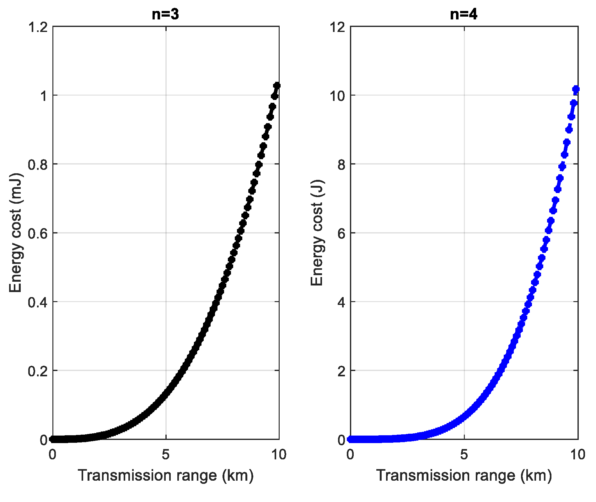
Using the parameters in Table 5, it was obtained as a function of the loss exponent (3 or 4), the energy levels shown in Figure 14. The results showed for transmission ranges up to 10 km, the maximum energy demand was 1.02 mJ in an environment with a loss exponent of 3 (which was the case of obstructed factories [61]), while the energy demand is above 10 J for n = 4 which would be the case with obstructed buildings [61]. In the rest of this paper, an exponent path loss of 3 was considered.

4.2. Management of the Harvested Energy

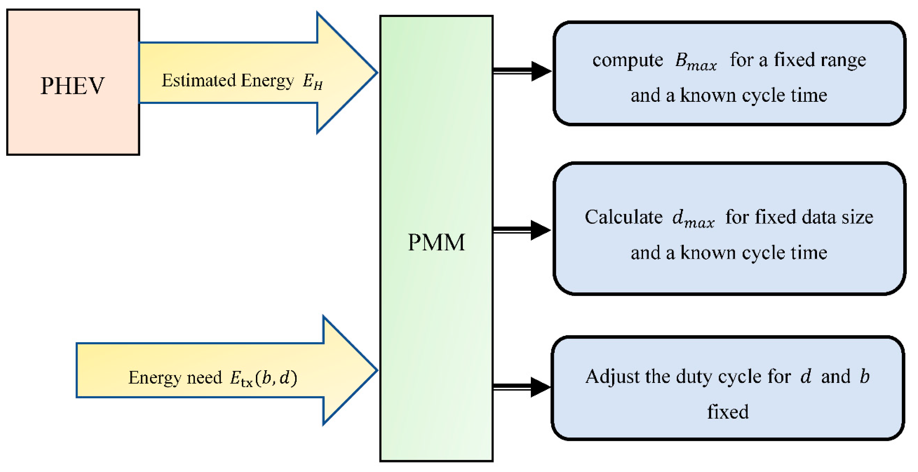
Equation (12) offers three possibilities of slaving the performance of the node to the energy harvested. These are the size $b$ of the data in the payload and the IWS’s transmission range. The third possibility is the transmission frequency in the case of a duty cycle adaptation strategy. Assuming that all the energy harvested is dedicated to the operation of the IWS (i.e., we consider an ideal case of a lossless harvesting circuit), the energy management module will then work as shown in Figure 15 below.

As shown in this figure, the objective is to transmit the maximum amount of data at the end of the cycle for a known measurement cycle time and distance. This first scenario makes it possible to reduce the length of the queue of data stored in the sensor [62]. In the second case, it is considered that the transmission of a data size is fixed in advance at the greatest possible distance; this strategy would be suitable for fairly dense mesh networks and minimize transmission delays due to multi-hop communications [63]. The duty cycle strategy is the third case dealt with; it applies when the data size and transmission range are previously defined. To simplify writing, for maximizing the data size, the used protocol will be abbreviated as MDSP. It will be a question for the PMM to use all of the harvested energy (estimated by the PHEV) during the current cycle to transmit data at the end of the cycle. Regarding the harvested energy stored during the measurement cycle, it is designated by $E_H$ and is defined as follows:

$$E_H = \underset{t}{\overset{t+T}{{\displaystyle \int }}}{p}_{\mathrm{PHEV}}\left(\tau \right)·d\tau$$

(13)

where $T$ is the duration of a cycle, $p_{\mathrm{PHEV}}$ is the harvestable power during the current measurement cycle; the PHEV predicts it, and $t$ is the instant marking the start of the current cycle.

The problem of optimizing energy management by the PMM is then the problem P1 formulated as follows:

$$\underset{b,d}{\min }\left(E_H - E_{WS}\left(b,d\right)\right) \mathrm{s}.\mathrm{t}. \{\begin{array}{c}{E}_{H_i} - E_{WS} \ge 0\\ b \ge 0 ;d \ge 0\end{array}$$

(14)

This problem boils down to minimizing the residual energy of the IWS at the end of each cycle while preventing it from going through a value less than 0. The node’s actual residual energy at the end of each measurement cycle, considering its accumulated energy, is defined as follow:

$$E_{\mathrm{residual}} = E_H - E_{WS}\left(b,d\right) + \underset{t}{\overset{t+T}{{\displaystyle \int }}}\left(p_{\mathrm{real}} - p_{\mathrm{PHEV}}\right)\left(\tau \right)·d\tau$$

where $p_{\mathrm{real}}$ is the power actually accumulated during the measurement cycle; the other parameters of the equation are defined as previously.

For data size analysis, it is assumed that the network is deployed at a fixed distance, $d$ from the base station. The measurement cycle is one minute, corresponding to the initial sampling of the vibration data. Figure 16 shows the operational flowchart of the PMM.

In Figure 16, $E_{min}$ is the minimum energy required to transmit a bit. At the start of the cycle, the range of data variations is defined, and the ranged and the duration $∆T$ of the cycle; $nT$ represents the number of samples taken during the month. The operation of PMM comes down to transmitting as much data as possible at the end of the cycle under the basis of the energy harvested during the cycle. The duty cycle adaptation is also considered in this algorithm because the IWS stays on standby mode if it has not accumulated the energy necessary to transmit a data bit. The transmission range was firstly set at 1 km, and the maximum data size that can be transmitted was 1500 bits. The results obtained in terms of cumulative data over one month are shown in Figure 17.

• Figure 17a shows the transmitted data accumulated over the month for a transmission range of $1 \mathrm{km}$. The result also highlights the frequency of transmission of the IWS. Overall, it was achieved that the IWS depletes its energy reserve during the first hours of measurement. For example, for a transmission with a maximum size of $4 \mathrm{kbits}$, the average throughput at the start of the month was 4.36 bits / s, unlike 0.5 bits / s observed towards the end of the month.
• In Figure 17b, the maximum range was increased to 3 km, and it is observed that the amount of data transmitted over the whole month decreases, which was an expected result since the energy cost of the IWS has increased.
• In Figure 17c, the transmission range varies from 100 to 5000 km, with a data size set to the legend’s values. The amount of data transmitted over the month increases with increasing packet size. For example, for packets of size 4096 bits, it was obtained that 94.21 kbits of data were transmitted during the month under the basis of the energy harvested from the vibrations. This amount of data corresponds to an average throughput of 2.15 bits per second.
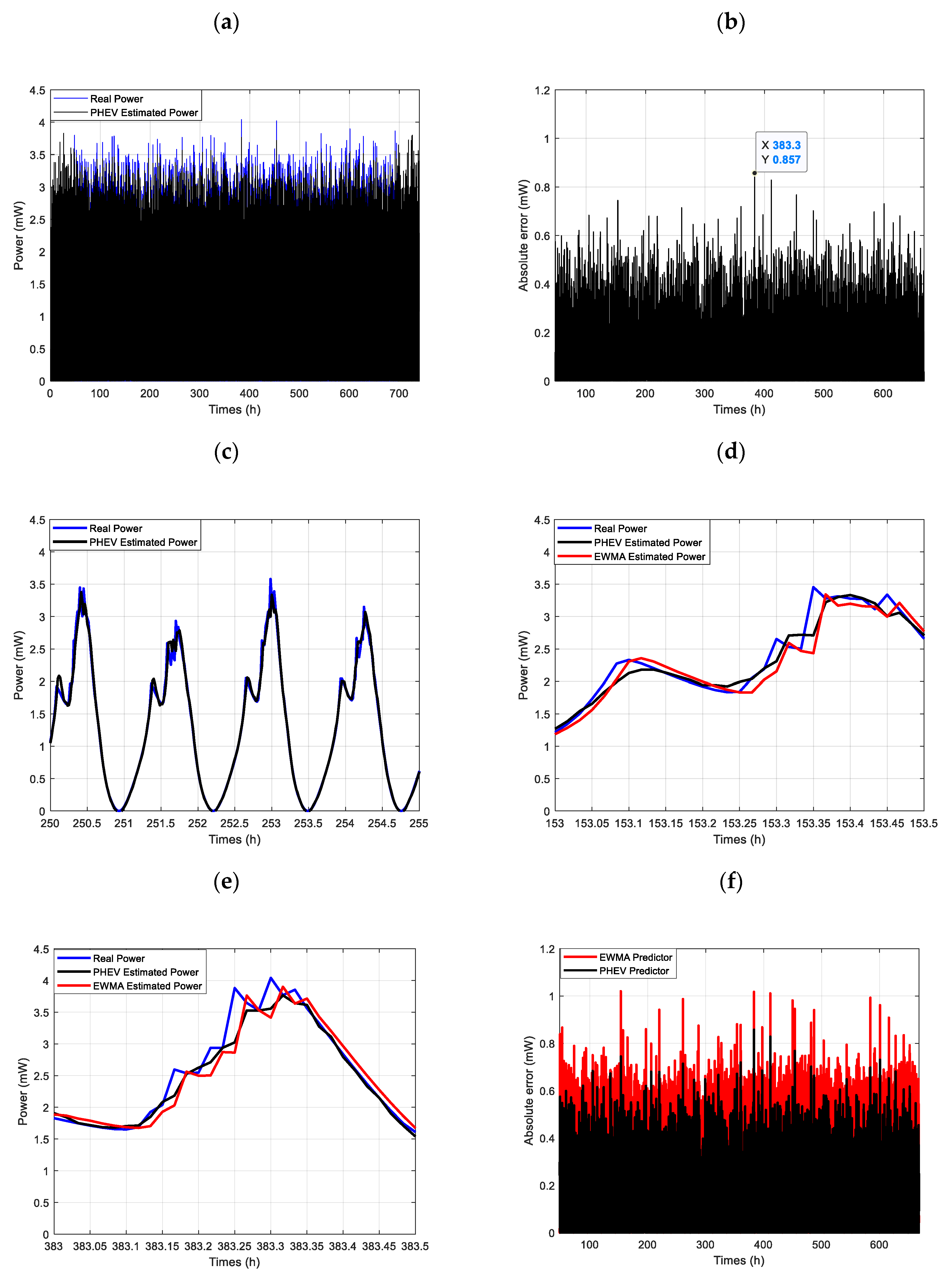
• For different packet sizes (512 bits, 1024 bits, 2048 bits, and 4096 bits), the evolution of the residual energy of the IWS is shown in Figure 17d. The evolution of the residual energy agrees with the previous results, in which it was noted that the transmission frequency is higher in the first hours of the month. It was also observed that the residual energy of the IWS increased after each transmission. This was justified because the harvestable energy calculation during each measurement cycle is based on the PHEV’s predicted power. This power was less than or equal to the real power, as shown in Figure 13a. This is another advantage of PHEV, which avoids overestimating the harvestable power, as is the EWMA predictor.

Overall, the achieved throughput based on the harvested energy can be satisfactory for monitoring temperature data, which varies very slowly due to thermal inertia. Note that the real throughput can also be improved if the residual energy of the IWS is updated after each transmission since, in most of the results obtained, the predicted energy is below the actual energy.

5. Comparison with Related Works

Very few works offer a complete design for IWSs powered by vibration energy. The complete design method includes the PT’s performance and defines the specifications of the IWS powered by the harvested energy, more specifically from vibrations.

Table 6. Comparison with some related designs.

Ref (Year)	Applications (Acceleration @ Frequency)	Used Method	Throughput @Transmission Range@ Transmission Frequency
[64] (2005)	$--@ 60 \mathrm{Hz}$	Data compression and HSU approach	− @ − @ $0.1 {\mathrm{s}}^{-1}$
[65] (2017)	$0.15 \mathrm{g} @ 40 \mathrm{Hz}$	HSU	− @ − @ $1 {\min }^{-1}$
[38] (2017)	$--@ 2.42 \mathrm{Hz}$	HSU	− @ − @ $12 {\mathrm{h}}^{-1}$
[66] (2018)	Vehicles $\left(1.3 \mathrm{g} @40 \mathrm{Hz}\right)$	HSU	$--@ 327 \mathrm{m} @ 10 {\min }^{-1}$
[19] (2020)	Mining locomotive $\left(0.98 \mathrm{g} @21.88 \mathrm{Hz}\right)$	PT with SSHI and HSU	1.21 bits/s @ 958 m @ 7${\min }^{-1}$
This Work (2020)	SAG	PT with PHEV and MDSP	$4 \mathrm{bits}/\mathrm{s}@3 \mathrm{km} @ 1{\min }^{-1}$

shows the comparison with some related designs. The application, as well as the strategy used, are also specified. This comparison was proposed in terms of throughput, transmission range, or else transmission frequency.

As shown in Table 6, the commonly used method is the Harvest-Store-Use technique, which involves leaving the IWS on standby until enough energy is harvested for data transmission. The design in [64] was one of the first to propose a slaving of sensor performance to harvestable energy. Although a transmission frequency of 10 Hz was reached in this work, it is important to mention that the data compression technique (which can cause loss of information) was used. Besides, the sensor was powered by a hybrid energy harvesting system comprising the PT and a photovoltaic cell.

In [65], a transmission frequency equal to that achieved in this work was obtained. However, these results are based on laboratory tests and not on an actual industrial application. The same observation can be made for the study in [38]. In [19] by considering most PT optimization solutions (in particular the SSHI technique), it is obtained that the vibrations took at a given moment in a mining locomotive make it possible to transmit data every 7 min at only 958 m, unlike every 1 min to 3 km as is the case in our study.

Overall, unlike our design method, most of the related designs are based on fixed excitation characteristics (constant frequency and constant acceleration) of the transducer, which is difficult to achieve in a real situation.

6. Conclusions

This paper is motivated by the need to deploy completely autonomous IWS in current industrial applications to support Industry 4.0 objectives. A design method is introduced here to make it possible to maximize the size of the transmitted data to the BS at each measurement cycle. Unlike most of the work, which consists of accumulating the harvested energy in a battery until it is enough to transmit data, this work proposes predicting the rate of the harvestable energy. The vibrations that abound in the industrial sector are a power source for the IWS. A database of the vibrations at the location of the IWS is first made up then the mechanical to electrical energy conversion is performed by using a Simscape model. Initially, linear prediction techniques based on the EWMA algorithm were considered. Although the results obtained were satisfactory, a relative prediction error of approximately 25.25% was obtained. It subsequently exploited the periodicity observed in the harvestable power, periodicity due to the industrial process’s repetitive tasks, to propose a PHEV, which made it possible to reduce the relative error to 21% and the RMSE from 28.6% to 19.5%. The energy predictor makes it possible, under the basis of a hardware block consumption model based on commonly used components, to ensure an average bit rate of 4 bits/s, which is satisfactory for observing physical phenomena such as temperature. The design method proposed here ensures the WS’s energy autonomy while maintaining an acceptable QoS and can be applied to any other industrial process.

References

1. Irina, K.; Pavel, L.; Nadezhda, Z.; Inna, S.; Gulnara, Y.; Elena, Z. Fourth Industrial Revolution-Engineering Innovations for Labor Productivity Increasing. J. Talent Dev. Excell. 2020, 12, 477–487. [Google Scholar]
2. Chen, M.; Wan, J.; González-Valenzuela, S.; Liao, X.; Leung, V.C. A Survey of Recent Developments in Home M2M Networks. IEEE Commun. Surv. Tutor. 2014, 16, 98–114. [Google Scholar] [CrossRef]
3. Doebling, S.W.; Farrar, C.R.; Prime, M.B.; Shevitz, D.W. Damage Identification and Health Monitoring of Structural and Mechanical Systems from Changes in Their Vibration Characteristics: A Literature Review; Los Alamos National Lab.: New Mexico, NM, USA, 1996. [Google Scholar]
4. Rai, V.; Mohanty, A. Bearing fault diagnosis using FFT of intrinsic mode functions in Hilbert–Huang transform. Mech. Syst. Signal Process. 2007, 21, 2607–2615. [Google Scholar] [CrossRef]
5. Felser, M. Real-time ethernet-industry prospective. Proc. IEEE 2005, 93, 1118–1129. [Google Scholar] [CrossRef]
6. Ehrlich, M.; Wisniewski, L.; Jasperneite, J. State of the art and future applications of industrial wireless sensor networks. In Kommunikation und Bildverarbeitung in der Automation; Springer: Cham, Switzerland, 2018; pp. 28–39. [Google Scholar]
7. Kadir, E.A.; Hu, A.P. A power processing circuit for indoor Wi-Fi energy harvesting for ultra-low power wireless sensors. Appl. Sci. 2017, 7, 827. [Google Scholar] [CrossRef] [Green Version]
8. Travassos, X.L.; Avila, S.; Grubisic, S.; Linhares, A.; Ida, N. Electromagnetic Field Exposure Assessment in a Multi Source Telecommunication Environment. Wirel. Pers. Commun. 2020, 110, 2213–2225. [Google Scholar] [CrossRef]
9. Twaha, S.; Zhu, J.; Yan, Y. Power conditioning of thermoelectric generated power using dc-dc converters: A case study of a boost converter. In Proceedings of the International Symposium of Heat Transfer and Heat Powered Cycles 2016, Nottingham, UK, 26–29 June 2016. [Google Scholar]
10. Li, X.; Li, D.; Wan, J.; Vasilakos, A.V.; Lai, C.-F.; Wang, S. A review of industrial wireless networks in the context of industry 4.0. Wirel. Netw. 2017, 23, 23–41. [Google Scholar] [CrossRef]
11. Lozoya-Santos, J.d.-J.; Félix-Herrán, L.; Tudón-Martínez, J.C.; Vargas-Martinez, A.; Ramirez-Mendoza, R.A. Design and implementation of an iot-oriented strain smart sensor with exploratory capabilities on energy harvesting and magnetorheological elastomer transducers. Appl. Sci. 2020, 10, 4387. [Google Scholar] [CrossRef]
12. Roundy, S.; Wright, P.K.; Rabaey, J. A study of low level vibrations as a power source for wireless sensor nodes. Comput. Commun. 2003, 26, 1131–1144. [Google Scholar] [CrossRef]
13. Covaci, C.; Gontean, A. Piezoelectric energy harvesting solutions: A review. Sensors 2020, 20, 3512. [Google Scholar] [CrossRef]
14. Guyomar, D.; Badel, A.; Lefeuvre, E.; Richard, C. Toward energy harvesting using active materials and conversion improvement by nonlinear processing. IEEE Trans. Ultrason. Ferroelectr. Freq. Control 2005, 52, 584–595. [Google Scholar] [CrossRef] [PubMed] [Green Version]
15. Angelov, P.; Nielsen-Lönn, M. A Fully Integrated Multilevel Synchronized-Switch-Harvesting-on-Capacitors Interface for Generic PEHs. IEEE J. Solid-State Circuits 2020, 55, 2118–2128. [Google Scholar] [CrossRef]
16. Lefeuvre, E.; Badel, A.; Richard, C.; Guyomar, D. Piezoelectric energy harvesting device optimization by synchronous electric charge extraction. J. Intell. Mater. Syst. Struct. 2005, 16, 865–876. [Google Scholar] [CrossRef]
17. Richard, C.; Guyomar, D.; Audigier, D.; Ching, G. Semi-passive damping using continuous switching of a piezoelectric device. In Proceedings of the Smart Structures and Materials 1999: Passive Damping and Isolation, Newport Beach, CA, USA, 1 March 1999; pp. 104–112. [Google Scholar]
18. Won, C.C.; Sulla, J.L.; Sparks, D.W.; Belvin, W.K. Application of piezoelectric devices to vibration suppression. J. Guid. Control Dyn. 1994, 17, 1333–1338. [Google Scholar] [CrossRef]
19. Mouapi, A.; Hakem, N.; Kandil, N. Cantilevered Piezoelectric Micro Generator Design Issues and Application to the Mining Locomotive. Energies 2020, 13, 63. [Google Scholar] [CrossRef] [Green Version]
20. Liang, J.; Liao, W.-H. Improved design and analysis of self-powered synchronized switch interface circuit for piezoelectric energy harvesting systems. IEEE Trans. Ind. Electron. 2011, 59, 1950–1960. [Google Scholar] [CrossRef]
21. Chandwani, J.; Somkuwar, R.; Deshmukh, R. Multi-band piezoelectric vibration energy harvester for low-frequency applications. Microsyst. Technol. 2019, 25, 3867–3877. [Google Scholar] [CrossRef]
22. Shi, G.; Xia, Y.; Yang, Y.; Chen, J.; Peng, Y.; Xia, H.; Wang, X.; Qian, L. A Sensor-less Self-tuning Resonance System for Piezoelectric Broadband Vibration Energy Harvesting. IEEE Trans. Ind. Electron. 2020. [Google Scholar] [CrossRef]
23. Choudhary, P.; Bhargava, L.; Singh, V.; Choudhary, M.; Kumar Suhag, A. A survey–Energy harvesting sources and techniques for internet of things devices. Mater. Today 2020. [Google Scholar] [CrossRef]
24. Kwon, K.; Yang, J.; Yoo, Y. Adaptive control of the packet transmission period with solar energy harvesting prediction in wireless sensor networks. Sensors 2015, 15, 9741–9755. [Google Scholar] [CrossRef] [Green Version]
25. Herrería-Alonso, S.; Suárez-González, A.; Rodríguez-Pérez, M.; Rodríguez-Rubio, R.F.; López-García, C. A solar altitude angle model for efficient solar energy predictions. Sensors 2020, 20, 1391. [Google Scholar] [CrossRef] [PubMed] [Green Version]
26. Kansal, A.; Hsu, J.; Zahedi, S.; Srivastava, M.B. Power management in energy harvesting sensor networks. TECS 2007, 6, 32-es. [Google Scholar] [CrossRef]
27. Yi, Z.; Yang, B.; Zhang, W.; Wu, Y.; Liu, J.-Q. Batteryless Tire Pressure Real-Time Monitoring System Driven by an Ultralow-frequency Piezoelectric Rotational Energy Harvester. IEEE Trans. Ind. Electron. 2020. [Google Scholar] [CrossRef]
28. Instruments, T. A True System-on-Chip Solution for 2.4 GHz IEEE 802.15.4/ZigBee CC2430. Available online: https://www.ti.com/product/CC2430 (accessed on 17 November 2020).
29. Devices, A. Small, Low Power, 3-Axis ±5 g Accelerometer. Available online: https://www.analog.com/media/en/technical-documentation/data-sheets/ADXL325.pdf (accessed on 17 November 2020).
30. Instruments, T. MSP430G2x53 MSP430G2x13 MIXED SIGNAL MICROCONTROLLER. Available online: https://www.ti.com/product/MSP430G2553 (accessed on 17 November 2020).
31. ST. STLM20 Ultra-Low Current 2.4 V Precision Analog Temperature Sensor. Available online: https://www.st.com/resource/en/datasheet/stlm20.pdf (accessed on 17 November 2020).
32. Instruments, T. MSP430L092 MSP430C09x MIXED SIGNAL MICROCONTROLLER. Available online: https://www.ti.com/lit/pdf/slas673 (accessed on 17 November 2020).
33. Instruments, T. CC2520 DATASHEET 2.4 GHZ IEEE 802.15.4/ZIGBEE® RF TRANSCEIVER. Available online: https://www.ti.com/product/CC2520#:~:text=The%20CC2520%20is%20TI’s%20second,C%20and%20low%20voltage%20operation (accessed on 17 November 2020).
34. NXP. MPL115A1 Miniature SPI Digital Barometer, 50 to 115 kPa. Available online: https://www.nxp.com/products/sensors/pressure-sensors/barometric-pressure-15-to-115-kpa/50-to-115kpa-absolute-digital-pressure-sensor:MPL115A (accessed on 17 November 2020).
35. Atmel. 8-Bit Atmel Microcontroller with 128KBytes In-System Programmable Flash ATmega128 ATmega128L. Available online: http://ww1.microchip.com/downloads/en/DeviceDoc/doc2467.pdf (accessed on 17 November 2020).
36. Semtech. SX1211 Transceiver Ultra-Low Power Integrated UHF Transceiver. Available online: https://www.semtech.com/products/wireless-rf/fsk-transceivers/sx1211 (accessed on 17 November 2020).
37. MIDÉ. Packaged Piezoelectric Actuators and Sensors. Available online: https://www.mide.com/collections/vibration-energy-harvesting-with-protected-piezos (accessed on 23 December 2018).
38. Ma, Y.; Ji, Q.; Chen, S.; Song, G. An experimental study of ultra-low power wireless sensor-based autonomous energy harvesting system. J. Renew. Sustain. Energy 2017, 9, 054702. [Google Scholar] [CrossRef]
39. Cottone, F. Introduction to Vibration Energy Harvesting. Available online: https://www.nipslab.org/files/nips%20summer%20school%202011/Cottone%20Introduction%20to%20vibration%20harvesting.pdf (accessed on 5 August 2011).
40. Mechatronics, C.T.I.I. Piezo Actuators. Available online: https://www.googleadservices.com/pagead/aclk?sa=L&ai=DChcSEwjDxq_4rrbfAhWVW4YKHQWeB-gYABAAGgJ2dQ&ohost=www.google.ca&cid=CAESEeD2gaWdpvwQojpjcabhUnBJ&sig=AOD64_2yDl2hSIleDK4dIP8DPbXou5MIqQ&q=&ved=2ahUKEwiDz6n4rrbfAhUS1VkKHRAzAhgQ0Qx6BAgLEAE&adurl (accessed on 23 December 2018).
41. Intellys. Predictive Maintenance Solutions. Available online: https://www.microgensystems.com/ (accessed on 23 December 2018).
42. Perpetuum. Vibration Energy Harvesters. Available online: https://perpetuum2016.files.wordpress.com/2016/09/perpetuum-ltd-vibration-energy-harvester-data-sheet-21october2013.pdf (accessed on 23 December 2018).
43. Xu, S.; Gao, Y.; Zhou, G.; Mao, G. A Global Maximum Power Point Tracking Algorithm for Photovoltaic Systems Under Partially Shaded Conditions Using Modified Maximum Power Trapezium Method. IEEE Trans. Ind. Electron. 2020, 68, 370–380. [Google Scholar] [CrossRef]
44. Smits, J.G.; Choi, W.-S. The constituent equations of piezoelectric heterogeneous bimorphs. IEEE Trans. Ultrason. Ferroelectr. Freq. Control 1991, 38, 256–270. [Google Scholar] [CrossRef] [PubMed]
45. Shevtsov, S.; Flek, M. Random vibration energy harvesting by piezoelectric stack charging the battery. Procedia Eng. 2016, 144, 645–652. [Google Scholar] [CrossRef] [Green Version]
46. Sharma, G.; Singh, P.K.; Shrivastava, L. Autonomous Vehicle Power Scavenging Analysis for Vehicular Ad Hoc Network. In Proceedings of the International Conference on Intelligent Computing and Smart Communication 2019, Tehri, India, 20–21 April 2019; pp. 879–887. [Google Scholar]
47. MIDÉ. Quickpack Packaged Piezoelectric Actuators and Sensors. Available online: https://www.electronicsdatasheets.com/download/52778c8de34e240e07514237.pdf?format=pdf (accessed on 10 January 2014).
48. Bouguera, T.; Diouris, J.-F.; Andrieux, G.; Chaillout, J.-J.; Jaouadi, R. A novel solar energy predictor for communicating sensors. IET Commun. 2018, 12, 2145–2149. [Google Scholar] [CrossRef]
49. Piorno, J.R.; Bergonzini, C.; Atienza, D.; Rosing, T.S. Prediction and management in energy harvested wireless sensor nodes. In Proceedings of the 2009 1st International Conference on Wireless Communication, Vehicular Technology, Information Theory and Aerospace & Electronic Systems Technology, Aalborg, Denmark, 17 May 2009; pp. 6–10. [Google Scholar]
50. Cox, D.R. Prediction by exponentially weighted moving averages and related methods. J. R. Stat. Soc. Ser. B 1961, 23, 414–422. [Google Scholar] [CrossRef]
51. Halgamuge, M.N.; Zukerman, M.; Ramamohanarao, K.; Vu, H.L. An estimation of sensor energy consumption. Prog. Electromagn. Res. 2009, 12, 259–295. [Google Scholar] [CrossRef] [Green Version]
52. Razzaque, M.A.; Dobson, S. Energy-efficient sensing in wireless sensor networks using compressed sensing. Sensors 2014, 14, 2822–2859. [Google Scholar] [CrossRef] [PubMed] [Green Version]
53. Heinzelman, W.B.; Chandrakasan, A.P.; Balakrishnan, H. An application-specific protocol architecture for wireless microsensor networks. IEEE Trans. Wirel. Commun. 2002, 1, 660–670. [Google Scholar] [CrossRef] [Green Version]
54. Roy, N.R.; Chandra, P. Energy dissipation model for wireless sensor networks: A survey. Int. J. Inf. Technol. 2019, 12, 1343–1353. [Google Scholar] [CrossRef]
55. Mekki, K.; Bajic, E.; Chaxel, F.; Meyer, F. A comparative study of LPWAN technologies for large-scale IoT deployment. ICT Express 2019, 5, 1–7. [Google Scholar] [CrossRef]
56. Poluektov, D.; Polovov, M.; Kharin, P.; Stusek, M.; Zeman, K.; Masek, P.; Gudkova, I.; Hosek, J.; Samouylov, K. On the Performance of LoRaWAN in Smart City: End-Device Design and Communication Coverage. In Proceedings of the International Conference on Distributed Computer and Communication Networks, Moscow, Russia, 23–27 September 2019; pp. 15–29. [Google Scholar]
57. Mekki, K.; Bajic, E.; Chaxel, F.; Meyer, F. Overview of cellular LPWAN technologies for IoT deployment: Sigfox, LoRaWAN, and NB-IoT. In Proceedings of the 2018 IEEE International Conference on Pervasive Computing and Communications Workshops (Percom Workshops), Athens, Greece, 19–23 March 2018; pp. 197–202. [Google Scholar]
58. San Cheong, P.; Bergs, J.; Hawinkel, C.; Famaey, J. Comparison of LoRaWAN classes and their power consumption. In Proceedings of the 2017 IEEE symposium on communications and vehicular technology (SCVT), Leuven, Belgium, 14 November 2017; pp. 1–6. [Google Scholar]
59. Ochoa, M.N.; Guizar, A.; Maman, M.; Duda, A. Evaluating LoRa energy efficiency for adaptive networks: From star to mesh topologies. In Proceedings of the 2017 IEEE 13th International Conference on Wireless and Mobile Computing, Networking and Communications (WiMob), Rome, Italy, 9–11 October 2017; pp. 1–8. [Google Scholar]
60. Semtech. SX1280/SX1281/SX1282. Available online: https://www.semtech.com/products/wireless-rf/24-ghz-transceivers/sx1280#download-resources (accessed on 16 July 2020).
61. Rappaport, T.S. Wireless Communications: Principles and Practice; Prentice Hall PTR: New Jersey, NJ, USA, 1996; Volume 2. [Google Scholar]
62. Nobar, S.K.; Mansourkiaie, F.; Ahmed, M.H. Packet Dropping Minimization in Energy Harvesting-Based Wireless Sensor Network With Linear Topology. IEEE Access 2020, 8, 38682–38691. [Google Scholar] [CrossRef]
63. Srikanth, N.; Neha, N.; Mamatha, K.; Adithya, P.; Rutvik, P. Enhanced Sleep/Awake Schedule with Multi-Hop Hierarchical Routing Algorithm for Wireless Sensor Networks. 2020. Available online: https://papers.ssrn.com/sol3/papers.cfm?abstract_id=3624701 (accessed on 24 November 2020).
64. Arms, S.W.; Townsend, C.; Churchill, D.; Galbreath, J.; Mundell, S. Power management for energy harvesting wireless sensors. In Proceedings of the Smart Structures and Materials 2005: Smart Electronics, MEMS, BioMEMS, and Nanotechnology, San Diego, CA, USA, 9 March 2005; pp. 267–275. [Google Scholar]
65. Han, Y.; Feng, Y.; Yu, Z.; Lou, W.; Liu, H. A study on piezoelectric energy-harvesting wireless sensor networks deployed in a weak vibration environment. IEEE Sens. J. 2017, 17, 6770–6777. [Google Scholar] [CrossRef]
66. Mouapi, A.; Hakem, N.; Kandil, N.; Kamani, G.V. Vibrational-Powered Vehicle’s Mesh Wireless Sensor Network: Performance Evaluation. In Proceedings of the 2018 IEEE International Conference on Environment and Electrical Engineering and 2018 IEEE Industrial and Commercial Power Systems Europe (EEEIC/I&CPS Europe), Palermo, Italy, 12–15 June 2018; pp. 1–5. [Google Scholar]
Figure 1. Conceptual view of the proposed system, which is comprised of a piezoelectric transducer (PT), Predictor of the Harvestable Energy from Vibrations (PHEV), Power Management Module (PMM), Industrial Wireless Sensors (IWS), and Base Station (BS).
Applsci 10 08486 g001
Figure 2. Functional diagram of the workflow of the design method.
Applsci 10 08486 g002
Figure 3. (a) accelerometer location on the Semi-Autogenous Grinding (SAG) drive diagram. (b) photograph of the accelerometer location.
Applsci 10 08486 g003
Figure 4. Time evolution of vibrations over the first ten days of March.
Applsci 10 08486 g004
Figure 5. Frequency distribution of the measured vibrations.
Applsci 10 08486 g005
Figure 6. Simulation diagram in Simscape.
Applsci 10 08486 g006
Figure 7. Dependence between the harvested power and load resistance.
Applsci 10 08486 g007
Figure 8. Harvestable power harvested over the first four days.
Applsci 10 08486 g008
Figure 9. Harvestable power on different days of the month: Highlighting the periodicity. (a) Measurement over the month; (b) Zoom between the second and the fourth day.
Applsci 10 08486 g009
Figure 10. Sum of the Mean Square Error (MSE) as a function of the weighting factor.
Applsci 10 08486 g010
Figure 11. Exponentially Weighted Moving-Average (EWMA) predictor performance. (a) Real and estimated power over the whole measurement period; (b) Absolute error over the whole measurement period. (c) Zoom between the 6th and 7th day. (d) Zoom between the 15th and the 16th day. (e) Estimated power and absolute error during the 6th day. (f) Estimated power and absolute error during the 15th day.
Applsci 10 08486 g011
Figure 12. Used data history to predict the harvestable power.
Applsci 10 08486 g012
Figure 13. PHEV performance compared to EWMA. (a) Real and estimated power over the whole measurement period; (b) Absolute error over the whole measurement period. (c) Comparison of real and PHEV predicted powers during the 10th day. (d) Comparison of real and predicted powers (PHEV and EWMA) during the 6th day. (e) Comparison of real and predicted powers (PHEV and EWMA) during the 15th day. (f) Comparison of absolute prediction errors for the two algorithms (EWMA and PHEV).
Applsci 10 08486 g013
Figure 14. Node energy dissipation versus transmission range for b = 512 bits.
Applsci 10 08486 g014
Figure 15. Proposed methods for efficient energy management of the harvested energy.
Applsci 10 08486 g015
Figure 16. Block diagram of proposed protocol: Maximizing Data Size Protocol (MDSP).
Applsci 10 08486 g016
Figure 17. Transmitted data analysis. (a) transmission range of 1 km. (b) transmission range of 3 km. (c) transmission range between 0.1 and 5 km. (d) residual energy.
Applsci 10 08486 g017