Minimization of Global Adjustment Charges for Large Electricity Customers Using Energy Storage—Canadian Market Case Study

Abstract
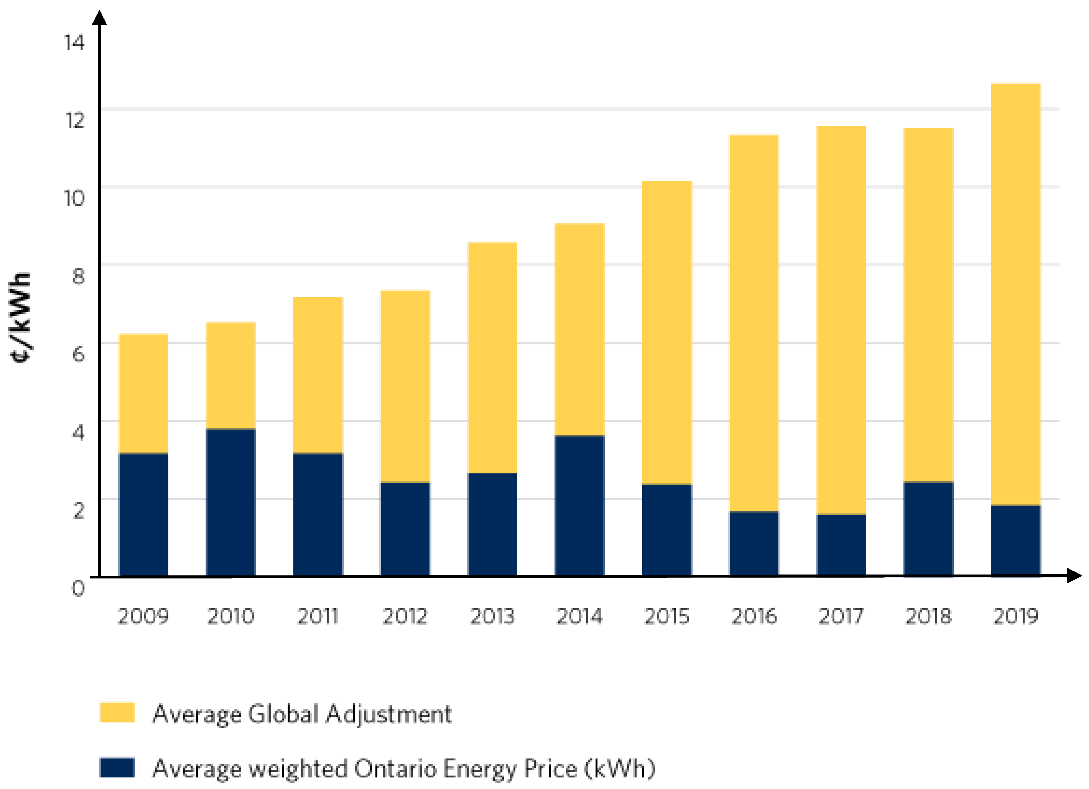
:1. Introduction
2. Profit-Maximizing Several Revenue Streams for a BESS
2.1. Major Objectives
- Objective function:
- Battery investment cost per year:
- The total customer energy cost per year (AEC):
- Cost of global adjustment per year (AGAC):
- The cost of demand charges per year (ADCC):
- Energy arbitrage revenue per year (ARVEA):
- Demand response revenue per year (ARVDR):
2.2. The Set of Constraint
- Hourly power of battery:
- Battery power at discharging mode:
- Battery power at charging mode:
- Peak demand factor (PDF):
- The battery intertemporal constrain:
- The life cycle limit:
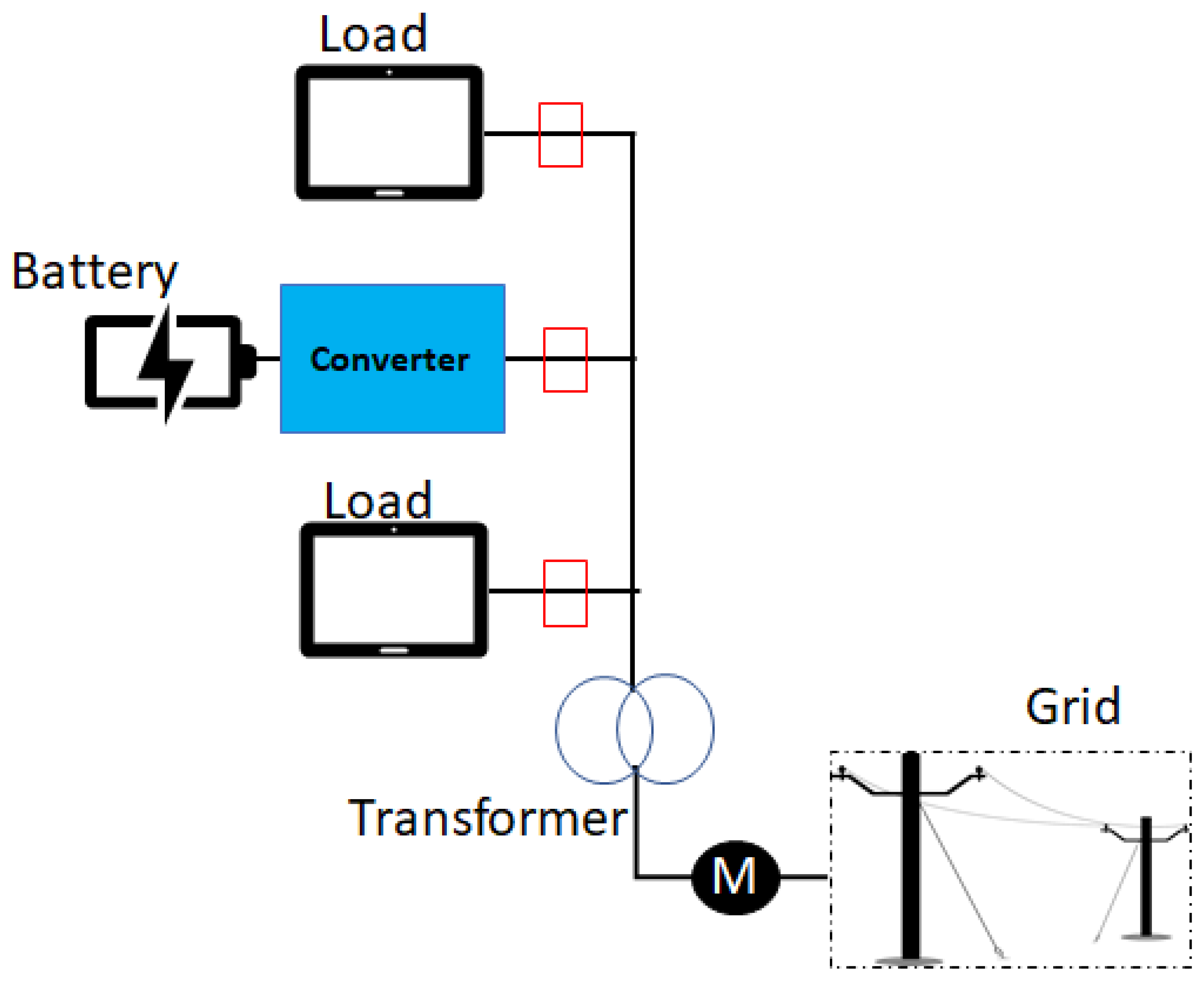
- Power balance constrain:
- The battery deployment during the considered set of peak hours:
- Limits to the battery capital cost:
- C-rate (ratio between and ):
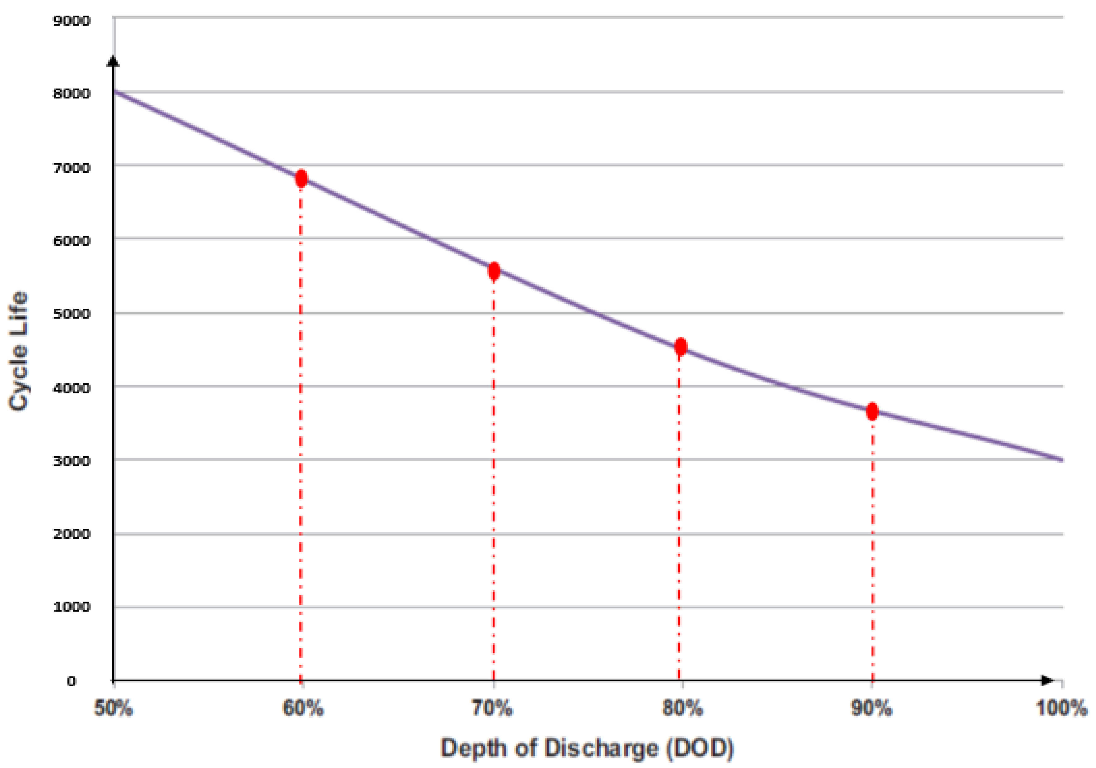
- Depth of discharge (DOD):
3. Solution Algorithm
| Algorithm 1 Battery storage scheduling for energy arbitrage maximization. | |
| 1. | Read all the model parameters including {, , r, Ny, } |
| 2. | Set , (small initial value), C-ratein = 0.5 |
| 3. | for |
| 4. | Calculate = where uph = 1, … where |
| 5. | Calculate where |
| 6. | if |
| 7. | , |
| 8. | else: |
| 9. | where |
| 10. | Return back to 6 |
| 11. | Calculate |
| 12. | for t |
| 13. | |
| 14. | else: |
| 15. | |
| 16. | for t W, |
| 17. | if && |
| 18. | = |
| 19. | else if && |
| 20. | ) = , |
| 21. | else: |
| 22. | |
| 23. | Calculate = |
| 24. | if |
| 25. | = , = & C-rate = |
| 26. | Return back the output values C-rate |
| 27. | Calculate |
| 28. | Calculate |
| 29. | Return back the output objective function = |
4. Results
4.1. Base Case Results
4.2. Comparison with the Results of the Developed Greedy Algorithm
4.3. Comparison with an Existing Sizing Problem for Energy Storage
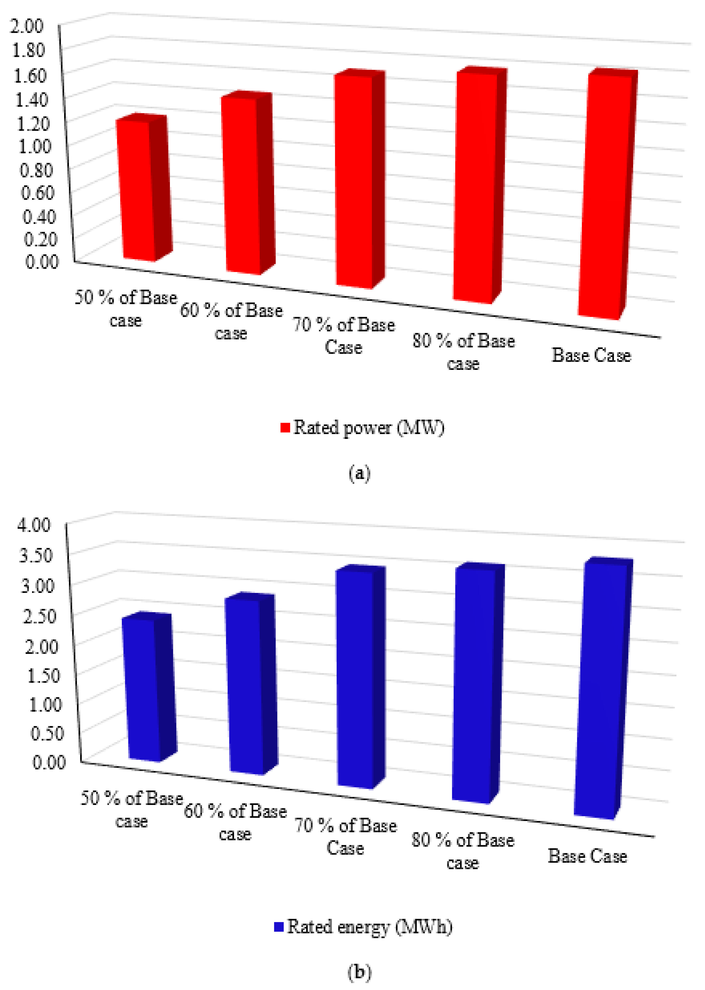
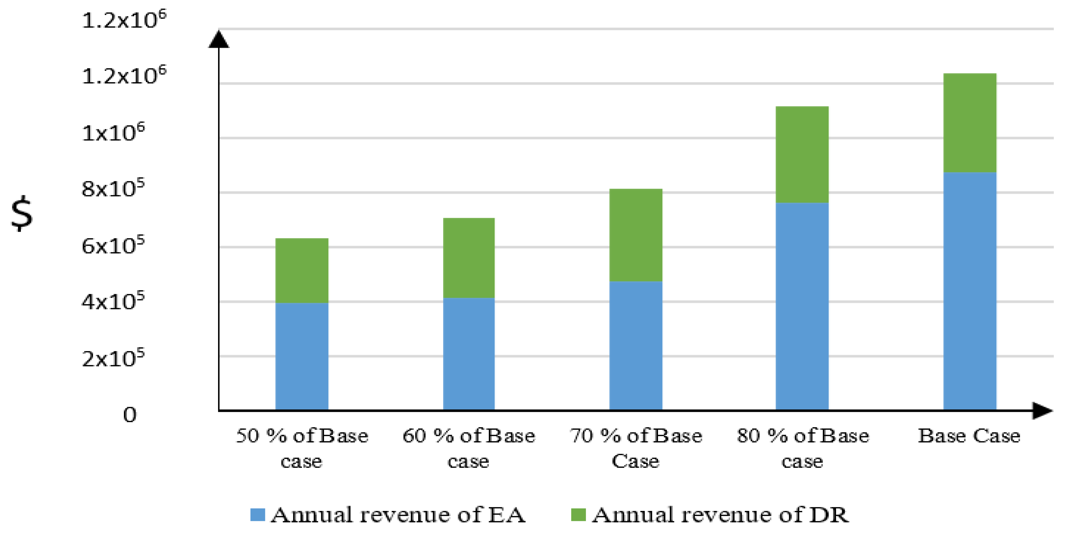
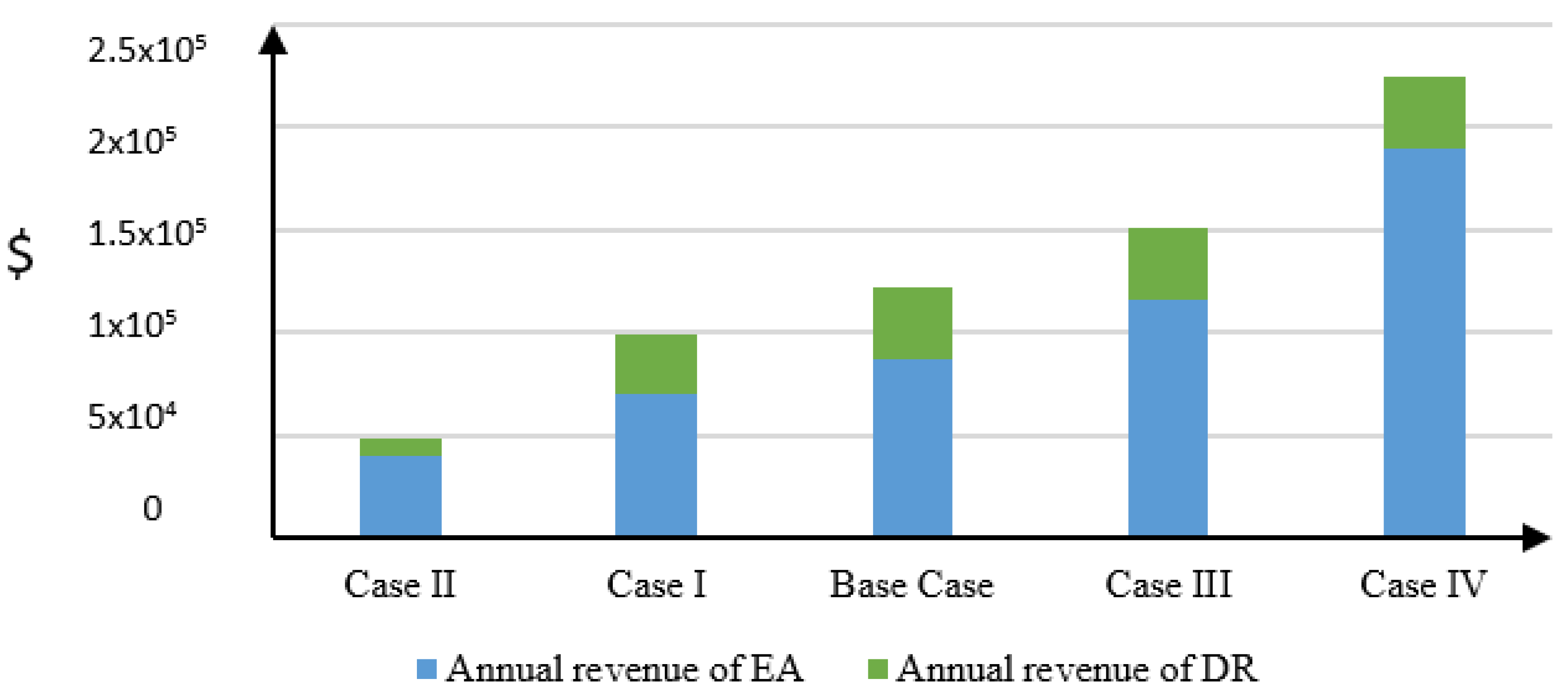
4.4. Sensitivity Case—Maximum Available Budget for Battery Purchasing
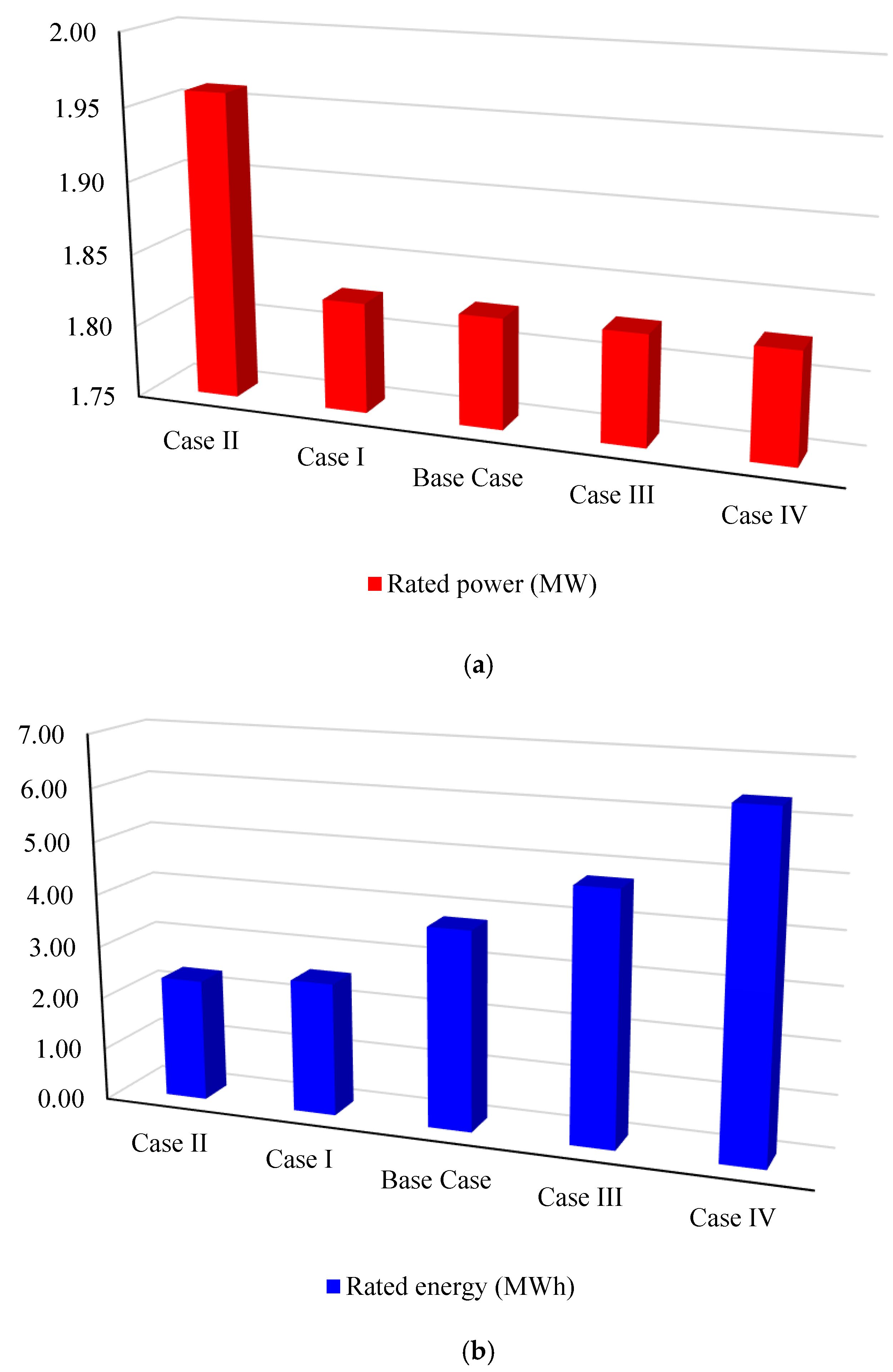
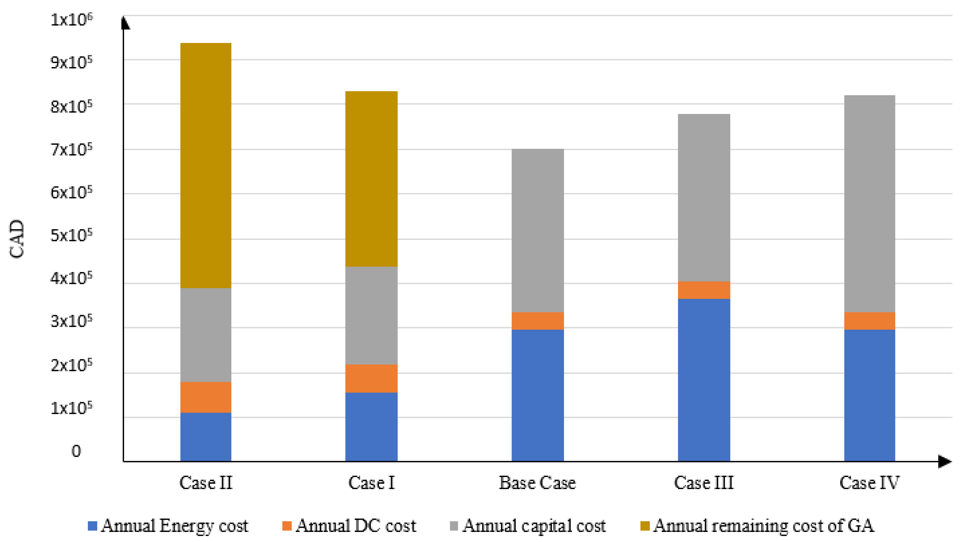
4.5. Sensitivity to C-Rate Results
5. Conclusions
Author Contributions
Funding
Conflicts of Interest
Nomenclature
| Indices | |
| T | Hourly index of the time |
| M | Monthly index of the time |
| Ph | Index of forecasted peaks |
| Q | Five coincident peaks for Ontario province, Canada |
| W | five-segments for the linearized depth of discharge (DOD) curve |
| Parameters | |
| Demand response power (decision variable) | |
| Spot price at t ($/MWh) | |
| Battery’s rated cycle life | |
| NC | Battery actual cycles life |
| Allowable maximum budget for the battery | |
| Battery cost factor for power | |
| Battery cost factor for energy | |
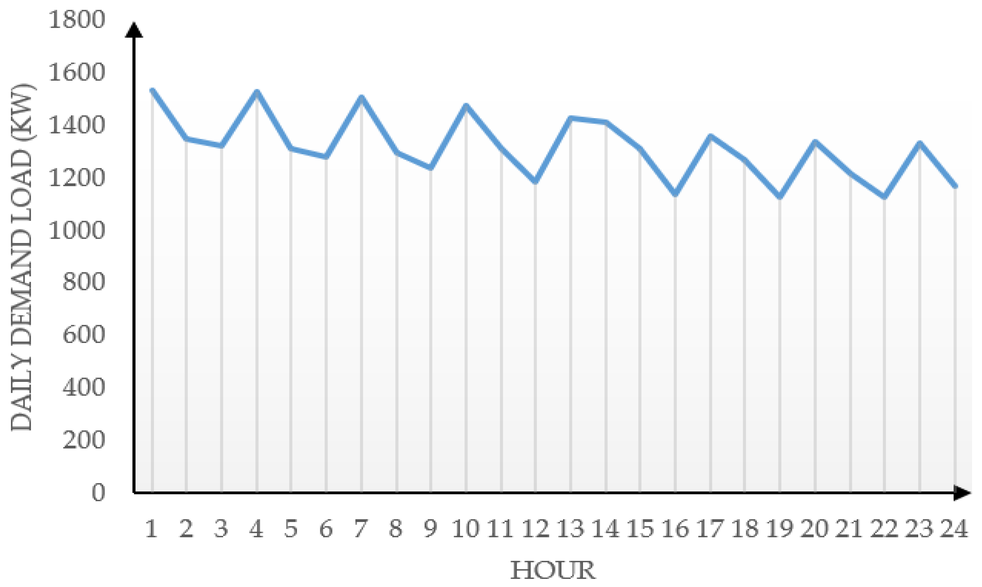
| Peak demand load for Ontario province | |
| Battery Crate () | |
| Total exchange power | |
| Power demand at t | |
| Charges for global adjustment per month | |
| Demand charges per month | |
| Battery efficiency (discharging) | |
| Battery efficiency (charging) | |
| Initial BESS energy value | |
| Demand response contract ($/Mw) | |
| Battery loading coefficient during the coincident peak hour | |
| R | Annual interest rate |
| Total number of operational years | |
| Linearization parameters of DOD curve | |
| Variables | |
| Batter capital cost per year ($/year) | |
| Total energy cost per year ($/year) | |
| Cost of global adjustment per year ($/year) | |
| Cost of the demand charge per year ($/year) | |
| Energy price arbitrage revenue per year ($/year) | |
| Demand response revenue per year ($/year) | |
| Battery maximum energy (MWh) (decision variable) | |
| Batter maximum power (MW) (decision variable) | |
| T | Time step |
| Depth of discharge of the battery. | |
| Hourly Battery power at t | |
| Discharging battery power at t (decision variable) | |
| Charging battery power at t (decision variable) | |
| Peak demand factor | |
| Set of the five peaks for the Ontario Jurisdiction | |
| Set of the forecasted peaks | |
| Integer variables | |
| Integer of the 5-segements of the linearized DOD curve | |
| Integer of battery discharging | |
References
- Eyer, J.M.; Corey, G.P.; Iannucci, J.J., Jr. Energy Storage Benefits and Market Analysis Handbook: A Study for the DOE Energy Storage Systems Program; Sandia National Laboratories: Albuquerque, NM, USA, 2004. [Google Scholar]
- Günter, N.; Marinopoulos, A. Energy storage for grid services and applications: Classification, market review, metrics, and methodology for evaluation of deployment cases. J. Energy Storage 2016, 8, 226–234. [Google Scholar] [CrossRef]
- Rau, N.S.; Tayor, B. A central inventory of storage and other technologies to defer distribution upgrades-optimization and economics. IEEE Trans. Power Deliv. 1998, 13, 194–202. [Google Scholar] [CrossRef]
- Venu, C.; Riffonneau, Y.; Bacha, S.; Baghzouz, Y. Battery storage system sizing in distribution feeders with distributed photovoltaic systems. IEEE Buchar. PowerTech 2019, 1–5. [Google Scholar] [CrossRef]
- Eyer, J.M. Electric Utility Transmission and Distribution Upgrade Deferral Benefits from Modular Electricity Storage: A Study for the DOE Energy Storage Systems Program; Sandia National Laboratories: Albuquerque, NM, USA, 2009. [Google Scholar]
- Zhang, T.; Emanuel, A.E.; Orr, J.A. Distribution feeder upgrade deferral through use of energy storage systems. In Proceedings of the 2016 IEEE Power and Energy Society General Meeting (PESGM), Boston, MA, USA, 17–21 July 2016; pp. 1–5. [Google Scholar]
- Hashmi, M.U.; Deka, D.; Busic, A.; Pereira, L.; Backhaus, S. Arbitrage with Power Factor Correction using Energy Storage. arXiv 2019, arXiv:1903.06132. [Google Scholar] [CrossRef] [Green Version]
- Lin, B.; Wu, W.; Bai, M.; Xie, C. Liquid air energy storage: Price arbitrage operations and sizing optimization in the GB real-time electricity market. Energy Econ. 2019, 78, 647–655. [Google Scholar] [CrossRef]
- Osorio, H.; Nasirov, S.; Agostini, C.A.; Silva, C. Assessing the economic viability of energy storage systems in the Chilean electricity system: An empirical analysis from arbitrage revenue perspectives. J. Renew. Sustain. Energy 2019, 11, 015901. [Google Scholar] [CrossRef]
- Nejad, S.; Gundogdu, B.M.; Gladwin, D.; Stone, D. Scheduling of grid tied battery energy storage system participating in frequency response services and energy arbitrage. IET Gener. Transm. Distrib. 2019, 13, 2930–2941. [Google Scholar]
- Terlouw, T.; AlSkaif, T.; Bauer, C.; van Sark, W. Multi-objective optimization of energy arbitrage in community energy storage systems using different battery technologies. Appl. Energy 2019, 239, 356–372. [Google Scholar] [CrossRef]
- Walawalkar, R.; Apt, J.; Mancini, R. Economics of electric energy storage for energy arbitrage and regulation in New York. Energy Policy 2007, 35, 2558–2568. [Google Scholar] [CrossRef]
- Neubauer, J.; Simpson, M. Deployment of Behind-the-Meter Energy Storage for Demand Charge Reduction; National Renewable Energy Lab. (NREL): Golden, CO, USA, 2015. [Google Scholar]
- McCormick, G.; Powell, R. Optimal pump scheduling in water supply systems with maximum demand charges. J. Water Resour. Plan. Manag. 2003, 129, 372–379. [Google Scholar] [CrossRef]
- Alsaidan, I.; Gao, W.; Khodaei, A. Battery energy storage sizing for commercial customers. In Proceedings of the 2017 IEEE Power & Energy Society General Meeting, Chicago, IL, USA, 16–20 July 2017; pp. 1–5. [Google Scholar]
- Chua, K.H.; Lim, Y.S.; Morris, S. Battery energy storage system for peak shaving and voltage unbalance mitigation. Int. J. Smart Grid Clean Energy 2013, 2, 357–363. [Google Scholar] [CrossRef]
- Ryu, B.; Makanju, T.; Lasek, A.; An, X.; Cercone, N. A Naive Bayesian Classification Model for Determining Peak Energy Demand in Ontario. In Smart City 360°; Springer: Berlin/Heidelberg, Germany, 2016; pp. 517–529. [Google Scholar]
- Jiang, Y.H.; Levman, R.; Golab, L.; Nathwani, J. Analyzing the impact of the 5CP Ontario peak reduction program on large consumers. Energy Policy 2016, 93, 96–100. [Google Scholar] [CrossRef]
- Jiang, Y.H.; Levman, R.; Golab, L.; Nathwani, J. Predicting peak-demand days in the Ontario peak reduction program for large consumers. In Proceedings of the 5th International Conference on Future Energy Systems, Cambridge, UK, 11–13 June 2014; pp. 221–222. [Google Scholar]
- IESO. What is Global Adjustment? Available online: http://www.ieso.ca/en/Learn/Electricity-Pricing/What-is-Global-Adjustment (accessed on 10 September 2020).
- IESO. Peak Tracker for Global Adjustment Class A. Available online: http://www.ieso.ca/Sector-Participants/Settlements/Global-Adjustment-for-Class-A (accessed on 10 September 2020).
- IESO. Average HOEP plus Average GA. Available online: http://www.ieso.ca/en/power-data/price-overview/global-adjustment (accessed on 10 September 2020).
- IESO. Global Adjustment Class A Eligibility. Available online: http://www.ieso.ca/en/Sector-Participants/Settlements/Global-Adjustment-Class-A-Eligibility (accessed on 10 September 2020).
- IESO Report: Hourly Ontario Energy Price (HOEP). Available online: http://www.ieso.ca/power-data/data-directory (accessed on 20 August 2020).
- IESO, Global Adjustment and Peak Demand Factor. Available online: http://www.ieso.ca/en/Sector-Participants/Settlements/Global-Adjustment-and-Peak-Demand-Factor (accessed on 20 August 2020).
- Annual Planning Outlook. Available online: http://www.ieso.ca/Sector-Participants/Planning-and-Forecasting/Annual-Planning-Outlook (accessed on 20 August 2020).
- Fourer, R.; Gay, D.M.; Kernighan, B.W. AMPL: A Modeling Language for Mathematical Programming, 2nd ed.; Brooks/Cole-Thomson Learning: Pacific Grove, CA, USA, 2003. [Google Scholar]


| Maximum allowable budget for the BESS () | $2.00 Million |
| Number of operational years (Ny) | 5 years |
| Battery power cost factor () | $125/kW |
| Battery energy cost factor () | $344/kWh |
| r (interest rate) | 6% |
| Less than half | |
| KD | 1.0 |
| Before | After | |
|---|---|---|
| Energy cost per year | $205,004.01 | $296,505.21 |
| Demand Charge cost per year | $42,470.00 | $40,375.86 |
| Global Adjustment cost per year | $860,176.24 | 0.0 |
| Capital cost per year | - | $363,604.81 |
| Revenue of Energy Price Arbitrage per year | - | $87,428.57 |
| Demand Response revenue per year | - | $35,164.28 |
| Saving of GAC per year | - | $860,176.24 |
| Total Annual bill | $1,107,650.25 | $700,485.88 |
| Existing BESS Sizing for DC [15] | Proposed Method | |
|---|---|---|
| Annual energy cost | $213,486.5 | $213,624.8 |
| Annual DC cost before BESS deployment | $206,418.0 | |
| Annual DC cost after BESS deployment | $158,672.0 | $157,946.0 |
| Annual Saving of DC | $47,746.00 | $48,472.00 |
| Annual BESS capital cost | $40,987.90 | $40,943.23 |
| BESS size | 352 KW | 356 KW |
| 374 KWh | 372 KWh | |
Publisher’s Note: MDPI stays neutral with regard to jurisdictional claims in published maps and institutional affiliations. |
© 2020 by the authors. Licensee MDPI, Basel, Switzerland. This article is an open access article distributed under the terms and conditions of the Creative Commons Attribution (CC BY) license (http://creativecommons.org/licenses/by/4.0/).
Share and Cite
Kadri, A.; Mohammadi, F.; Awadallah, M. Minimization of Global Adjustment Charges for Large Electricity Customers Using Energy Storage—Canadian Market Case Study. Appl. Sci. 2020, 10, 8585. https://doi.org/10.3390/app10238585
Kadri A, Mohammadi F, Awadallah M. Minimization of Global Adjustment Charges for Large Electricity Customers Using Energy Storage—Canadian Market Case Study. Applied Sciences. 2020; 10(23):8585. https://doi.org/10.3390/app10238585
Chicago/Turabian StyleKadri, Abdeslem, Farah Mohammadi, and Mohamed Awadallah. 2020. "Minimization of Global Adjustment Charges for Large Electricity Customers Using Energy Storage—Canadian Market Case Study" Applied Sciences 10, no. 23: 8585. https://doi.org/10.3390/app10238585
APA StyleKadri, A., Mohammadi, F., & Awadallah, M. (2020). Minimization of Global Adjustment Charges for Large Electricity Customers Using Energy Storage—Canadian Market Case Study. Applied Sciences, 10(23), 8585. https://doi.org/10.3390/app10238585