Abstract
Coverage path planning on a complex free-form surface is a representative problem that has been steadily investigated in path planning and automatic control. However, most methods do not consider many optimisation conditions and cannot deal with complex surfaces, closed surfaces, and the intersection of multiple surfaces. In this study, a novel and efficient coverage path-planning method is proposed that considers trajectory optimisation information and uses point cloud data for environmental modelling. First, the point cloud data are denoised and simplified. Then, the path points are converted into the rotation angle of each joint of the manipulator. A mathematical model dedicated to energy consumption, processing time, and path smoothness as optimisation objectives is developed, and an improved ant colony algorithm is used to solve this problem. Two measures are proposed to prevent the algorithm from being trapped in a local optimum, thereby improving the global search ability of the algorithm. The standard test results indicate that the improved algorithm performs better than the ant colony algorithm and the max–min ant system. The numerical simulation results reveal that compared with the point cloud slicing technique, the proposed method can obtain a more efficient path. The laser ablation de-rusting experiment results specify the utility of the proposed approach.
1. Introduction
Laser ablation has a wide range of applications in engineering [1]. This paper mainly focuses on the path planning methods of laser ablation. This kind of method has two main applications: One is laser surface treatment technology, the other is laser cleaning. Laser surface treatment technology has many branches, such as surface coating [2] and laser-induced periodic surface structures [3]. Laser cleaning also has a lot of applications [4]. Laser cleaning technology has the advantages of good cleaning effect, wide application range, high precision, non-contact type, and good accessibility. It is an environment-friendly cleaning technology with excellent development potential. In engineering, the manipulator is often used to carry a laser generator for processing.
Path planning plays a vital role in the control of a manipulator. Path planning can be classified into two independent subcategories: point-to-point path planning and coverage path planning [5]. In point-to-point path planning, the goal is to determine a collision-free path from a starting point to a destination point, optimising parameters such as time, distance, and energy. With the rise of autonomous driving and the broader application of mobile robots, point-to-point path planning has recently become an important topic in the field of robotics. Many methods have been used to solve the point-to-point path-planning problem. Zafar and Mohanta [6] categorised mobile robot path-planning strategies as classical methods and heuristic methods. Metaheuristic methods are more popular and widely used for the path planning of mobile robots [7].
Coverage path planning (CPP) is the task of determining a path that passes over all points of an area or volume while avoiding obstacles [8]. This task is integral to many robotic applications, such as agriculture and farming robots [5], cleaning robots [9], lawn mowers [10], autonomous underwater vehicles [11], unmanned aerial vehicles [12], and demining robots [13]. Generally, coverage algorithms are categorised as offline and online algorithms [14]. Offline coverage algorithms use fixed information, and the environment information is known in advance. In contrast, online algorithms do not assume full prior knowledge of the environment to be covered and utilise real-time sensor measurements to sweep the target space [15].
Furthermore, Khan et al. [16] summarised the coverage methods in three steps. The first step is to divide the environment into smaller regions (cells) for effective coverage. Then, the path planning of each subregion and the sequence planning among the subregions are performed according to the sweep direction. The last step is path smoothing.
There are several environmental decomposition methods, including cell-based decomposition techniques [17], grid-based methods [18], and spanning-tree-based coverage methods [19]. All these methods are based on the main concept of dividing the environment into different regions, similar to a regular region, to facilitate subsequent path planning. Regular paths are often used to cover each subregion, such as a spiral path [10] and a boustrophedon path [17].
Three main types of methods exist for sequence optimisation: greedy algorithms [20], dynamic programming [21], and evolutionary algorithms [22]. The purpose of this step is to determine the order in which different subregions are traversed and adjust the coverage path of each subregion if necessary.
Two path-smoothing method classes exist, namely, the graphical method [23] and the function-based method [24]. The main aim of path smoothing is to avoid having the robots stop, slow down, or reorient at sharper turns because path-planning algorithms, such as A *, D *, PRM, and RRT *, generate rectilinear (linear piecewise) paths for robots [25]. The graphical method uses simple shapes, such as circles and arcs, to generate a smooth path. In the function-based method, the path trajectory is represented by function equations, such as spirals and spline-based functions.
Many researchers have discussed the CPP problem. However, the state of the art needs to be significantly improved, particularly in terms of accuracy, efficiency, robustness, and optimisation [15]. The core idea of the above methods is to use regular curves or broken lines to traverse the fixed area, without considering many optimisation conditions. Typically, only the shortest route length or the smallest number of turns is considered. More importantly, because the global path is divided into multiple parts, the results of current methods are the superposition of multiple local optimal solutions, and not the global optimal solution.
Additionally, most methods only consider the problem of covering a continuous planar area. Such methods cannot deal with CPP on complex surfaces, closed surfaces, and intersections of multiple surfaces. These methods can be applied to CPP for cleaning robots, demining robots, and unmanned aerial vehicles, but not for machining robots.
To overcome the shortcomings of existing methods, in this study, the problem of path planning was examined from a different perspective. The primary purpose of path planning is to determine quickly the obstacle-free path that meets the requirements. Therefore, the path-planning process must include environmental modelling, optimisation objectives and boundary conditions, and optimisation methods.
In this study, point cloud data were used to model the working environment to improve the flexibility of planning, because point cloud data can be obtained in real time or in advance. More importantly, using point cloud data does not require environmental segmentation—data simplification is sufficient. Thus, the adaptability of this method is improved, which implies that the method can be used for CPP on complex surfaces, closed surfaces, and at the intersection of multiple surfaces. Using point cloud data lays the foundation for transforming the path-planning problem into an optimisation problem, thereby enabling this method to solve both the problems of CPP and point-to-point path planning.
Laser processing is characterised by a variable laser spot size. Another advantage of using the point cloud data is that it can work well with this characteristic. To ensure machining quality, people always expect that the curvature within the same laser spot range only has a small change. A larger spot size can be used to improve the efficiency at a position with a small curvature change. In contrast, a smaller spot size must be used to meet the machining requirements at a position with a large curvature change. After the point cloud is simplified, this problem can be formulated as a travelling salesman problem (TSP), which is an NP (non-deterministic polynomial)-hard problem. However, only a few scholars have conducted research based on this view. Xie et al. [26] developed two approaches to solve the CPP problem among multiple spatially distributed regions by considering the path planning in a single subregion as a CPP problem and the path planning between subregions as a TSP. However, this is similar to the sequence optimisation problem mentioned above. As the path of a single subregion needs to be adjusted multiple times, the algorithm complexity increases. Modares et al. [27] proposed a method to solve the CPP problem using multiple drones. The path planning of subregions is considered as a TSP, and the energy consumption is added to the optimisation goal. However, this method has been tested only in relatively simple environments.
Due to the similarity between CPP and TSP, in this study, an improved ant colony algorithm was used to solve the CPP problem to obtain an optimal path. Moreover, the trajectory optimisation information is added to obtain a more practical path for optimisation objectives because trajectory planning is often required after path planning in engineering practice. Simultaneously, the path smoothing is also achieved because the acceleration factor is added to the optimisation objective. On the other hand, using the inverse kinematics solution can transform the Cartesian space path planning into joint space trajectory planning. Thus, the manipulator can avoid losing control in the singular position because it is replaced once there exists a singular position.
The remainder of the article is structured as follows. In Section 2, the point cloud processing method is proposed. In Section 3, the fitness function is proposed. The improvement measures of the ant colony algorithm and the process of path planning are proposed in Section 4. Section 5 provides an analysis of the effectiveness of the proposed method using the simulation results. The conclusions are presented in Section 6. The content and function of each section are shown in Table 1.

Table 1.
Contents and functions of each section.
2. Point Cloud Pre-Processing
2.1. Point Cloud Denoising and Simplification
The point cloud is a dataset of points that have been used widely to represent shapes since the pioneering work of Alexa et al. [28]. The main focus of this study was on the application of the point cloud in path planning. Using the point cloud has several advantages. First, the point cloud data are easy to acquire—one scanner is sufficient. Moreover, the point cloud is suitable for complex geometries. Furthermore, it does not require global maintenance of the topology. The advantages of point-cloud-based methods over mesh-based methods are apparent when the workpiece is highly freeform and complex [28]. Finally, using a point cloud can skip the surface fitting process to generate the tool path directly, which is the idea of direct machining [29]. However, the use of the point cloud also has disadvantages. To improve the accuracy of the representation, the density of the point cloud data should typically be enormous. This increases the complexity of path planning. Therefore, before path planning, the point cloud data need to be processed to extract the required path points.
The problem of path planning using the point cloud has been investigated in many studies. Zhen et al. [30] demonstrated a point-cloud-based tool path generation algorithm using different tool path patterns previously designed. This method can reduce the path-planning complexity but limits the application of the method in complex geometries. Zou et al. [31] proposed a method for planning an isoparametric tool path from a point cloud and employed a point-based conformal map to build the parameterisation. However, the uneven spatial path reduces its efficiency. Masood et al. [32] developed an algorithm to generate tool paths for direct machining, including dividing the surface into ranges and generating B-spline curves within each range. However, the program is not equipped to handle surfaces with shapes other than a rectangle. Wang et al. [33] proposed a path-planning method based on a discontinuous grid partition algorithm using the point cloud for in situ printing and obtained a good printing effect. However, the influence of each parameter still needs further study. Zhang et al. [34] proposed a method for point cloud simplification, denoising, and boundary extraction based on a k-neighbourhood octree structure and applied it in grinding path planning.
In addition to the personalised methods described above, one common method is the point cloud slicing technique [35,36]. This method cuts the workpiece point cloud model through a series of parallel planes. Then, the adjacent points of the workpiece point cloud data near the two sides of each slice are matched to obtain the intersections between the matching points and slices. After each intersection is moved a certain distance along its normal vector, the processing path is obtained by connecting each point end to end. However, this method does not consider the path-planning problem as an optimisation problem. The path obtained is feasible but not optimal. Moreover, key parameters, such as cutting distance and direction, require artificial input, adding artificial factors to a certain extent.
Herein, a novel method is proposed for point cloud simplification based on a continuous grid partition. As the spot size of a laser is variable and the manipulator must remain at each position for at least 2 s during the processing to meet the ablation requirements, a dynamic mesh generation method is used. A larger spot size can be used to improve the efficiency at a position with a small curvature change. In contrast, a smaller spot size must be used to meet the machining requirements at a position with a large curvature change.
First, it is necessary to denoise the point cloud data. Methods such as median filter, mean filter, and Gaussian filter change the original point cloud data and reduce the accuracy. Therefore, a point cloud filtering method based on the k-nearest neighbours (k-NN) algorithm is proposed. The k-NN algorithm can determine the k closest points of a point. Then, the distances between this point and its k closest points are calculated. Once all the distances become significantly large, this point is considered as an error point.
Then, the point cloud data are transformed into structured point cloud data for path point extraction by projecting all the points onto the X-Y plane. A 2D mesh (grid) of points is prepared by computing extents (minimum and maximum) of the projected coordinates of the X-Y plane. The grid sizes are computed using a recursive method. First, the mesh is divided using a larger side length. Then, a plane fit is performed in each mesh, and its residual is calculated. If the residual is lesser than the accuracy requirement, meshing is performed at this location. If it is greater than the accuracy requirement, the mesh is subdivided with a smaller side length until all the grid points meet the accuracy requirement. Each grid point is a path point. Thereby, the fitted value and the grid point normal vector are obtained. The grid size is the spot size.
The size of the grid is related to the accuracy requirement and is influenced by the processing methods and machining accuracy, requiring specific analysis. If there are other constraints, restrictions on the normal vector and grid size are added.
Figure 1 illustrates the path point extraction flowchart, and Figure 2 depicts the effect of point cloud data processing (only considering the accuracy requirement).
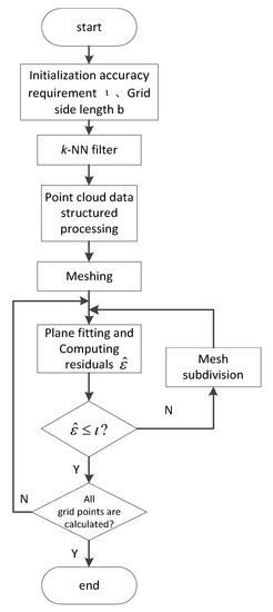
Figure 1.
Path point extraction process.
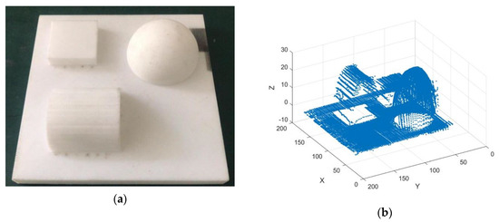
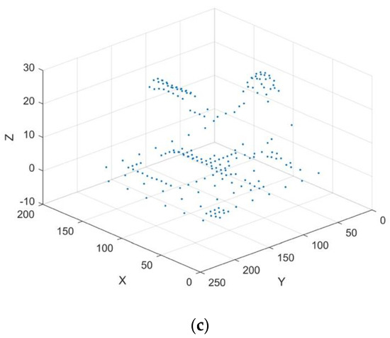
Figure 2.
Effect of point cloud data preprocessing: (a) sample piece model, (b) original scan data of the sample piece, and (c) extracted path points.
2.2. Inverse Kinematics
Figure 3 depicts a six-degree-of-freedom (6-DOF) serial manipulator.
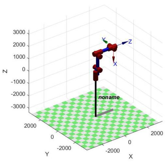
Figure 3.
Six-degree-of-freedom (6-DOF) serial manipulator.
To describe the dynamic information of the manipulator during operation, the 3D point coordinates in the point cloud data must be converted into the joint angle of the manipulator at the corresponding position. The iterative solution method is used.
A corresponding manipulator motion formula is needed in the solution process, and the key is the Denavit-Hartenberg (DH) parameters. The DH parameters express the position and angle relationship between two pairs of joint links with four parameters. The DH parameters of the manipulator depicted in Figure 3 are presented in Table 2.
Table 2.
Manipulator Denavit-Hartenberg (DH) parameters.
In the spatial neighbourhood of the joint rotation angle, the mapping relationship between the manipulator’s pose and the manipulator’s joint rotation angle can be considered linear. Therefore, the Jacobian matrix of the manipulator can be used to establish the relationship between the difference motion vector of the manipulator and the joint angle increments, such that the inverse kinematics gradually converge to an exact solution. To make the iteration converge, the iteration compensation decreases as the number of iterations increases until a solution that satisfies the convergence condition is obtained.
The Jacobian matrix J can establish the relationship between the joint speeds and the speed of the manipulator end-effector.
where v is the generalised velocity vector of the manipulator end-effector, J is the Jacobian matrix of the manipulator, which is a function of the manipulator joint rotation angle θ, and ω is a generalised velocity vector of each joint rotation angle.
By replacing the differential with the difference, the relationship between the differential motion vector of the manipulator in a certain spatial neighbourhood and the increment of the joint rotation angle can be obtained.
where Δθ is the increment of the joint rotation angle corresponding to different poses, and D is the differential motion vector, which is calculated based on the differential motion matrix.
The calculation of the differential motion matrix is as follows:
The differential motion matrix elements and the elements of the differential motion vector D have a corresponding relationship shown in Formula (5). After calculating the differential motion matrix according to Formula (4), each element in D can be calculated according to Formula (5).
The relative rotation angles of each joint from the current pose to the target pose in the spatial neighbourhood can be calculated using Equation (2). When the Jacobian matrix is singular in the iterative process, it can be solved by using the generalised inverse matrix instead. Using Equation (2) for iteration can lead to a situation wherein the iterative compensation is significantly large and leads to nonconvergence. Thus, the idea of learning rate exponential decay in machine learning is introduced. Then, the iterative formula is as shown in Equation (6).
Here, α(t) decays exponentially with the number of iterations, as shown in Equation (7).
where k indicates the current iteration number of the algorithm, K indicates the maximum iteration number, α0 is the initial value, and αK is the parameter value in the K-th iteration.
The flowchart of the inverse kinematics iterative algorithm is depicted in Figure 4.
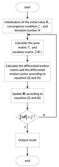
Figure 4.
The Inverse kinematics iterative algorithm flowchart.
The manipulator must remain at each position for at least 2 s during the processing to meet the ablation requirements. Once a singular position is obtained in the solution process, the mesh is subdivided again at that position according to the dynamic mesh generation method mentioned before, such that the manipulator can avoid stopping at the singular position during the machining process.
3. Optimisation Objective
The trajectory optimisation information is considered to obtain a more practical path for optimisation objectives because trajectory planning is often required after path planning in engineering practice. Most methods currently consider path planning and trajectory planning separately, which may cause the following problems. One is that the path may have to be adjusted to avoid the singular position after the path is generated in some cases, and this significantly reduces the effect of path planning. Another is that the optimal trajectory may not be generated by the shortest path because the optimisation objectives of path planning and trajectory planning are not the same. Therefore, it is necessary to consider path-planning and trajectory-planning information comprehensively. The optimisation objectives of optimal trajectory planning can be roughly classified into four categories: time optimal [37], energy optimal [38], jerk optimal [39], and hybrid optimisation. There are many different criteria of hybrid optimisation, such as smooth and time optimal [40], time–jerk optimal [41], and time acceleration jerk hybrid optimal [42].
In general, a process that consumes as little time and energy as possible and prevents the robot from making a sudden stop or a large turn is desired. The ideal solution is to generate a path, use that path for global trajectory planning, and evaluate the path by combining path information and trajectory information. However, this requires considerable computing resources and time, which is unacceptable. Therefore, an alternative solution of introducing time, energy, and acceleration factors into path planning in a relatively simple way is adopted. In this method, the computational complexity is reduced, and the optimal or better trajectory can be obtained based on prior information.
In the actual control of the manipulator, in addition to providing an exact path, it is also necessary to provide the time or speed information between every two consecutive path points. As the motion of all joints of the manipulator is considered, the inverse kinematics must be performed first to determine the rotation angle of each joint at each path point. Moreover, some restrictions must be considered when planning the path for the manipulator, including the maximum joint speed and maximum joint driving force or torque for each joint.
The difference method is used to calculate the joint displacement, velocity, acceleration, and jerk. The relationship between the angular velocity of the i-th joint and running time is given in Equation (8).
where n is the number of path points, is the joint rotation angle, and is the running time between two points.
The angular acceleration of the i-th joint is
The angular jerk of the i-th joint is
The energy consumption of the i-th joint is as follows:
where I is the moment of inertia.
To avoid the influence of the positive and negative of the acceleration and jerk, the squaring formula in Equation (9) is used, along with Equation (10), to obtain the expression of the optimisation objective.
where the manipulator running time function c1 is as follows:
The manipulator energy consumption function c2 is
The manipulator joint jerk function c3 is as follows:
The manipulator joint acceleration function c4 is
In the objective function and constraints above, F is the fitness function, is the weight coefficient, is the normalisation coefficient, and are the maximum speed and maximum driving torque of the i-th joint, respectively, and and represent the safety factors.
In this way, the optimisation objective is transformed into a function of time. For different task objects and task demands, more types of path shape can be obtained by adjusting the weight coefficients’ concrete value and normalisation coefficients.
4. Improved Ant Colony Algorithm
4.1. Basic Ant Colony Algorithm
With the development of numerous metaheuristic algorithms, many scholars have applied these algorithms to solve the path or trajectory optimisation problems. Due to the similarity between CPP and TSP, in this study, an improved ant colony algorithm was adopted to solve the CPP problem to determine an optimal path. The ant colony optimisation (ACO) algorithm is a heuristic random search algorithm based on a distributed autocatalytic process by simulating the collective path-seeking behaviour of ants in nature [43]. In comparison with other metaheuristic algorithms, the ant colony algorithm has the advantages of strong robustness, parallelism, and positive feedback. It has been widely used in path-planning problems.
There are two essential steps in simulating the foraging behaviour of the ant colony. The first is counting the transition probability from one point to another, according to Equation (17). The second is updating the pheromone according to Equation (18).
where is a point set of allowed from point i, is the pheromone between point i and point j, and is the visibility, which is generally . Moreover, α and β are parameters that control the relative importance of the trail pheromone versus visibility.
where is a parameter, denotes the evaporation of the trail pheromone between time and , and follows Equation (19).
where is the amount per iteration of the path of the trail pheromone laid on the edge (i,j) by the k-th ant between time and . It follows Equation (20):
where is a constant, and is the tour length of the k-th ant.
4.2. Improved Max–Min Ant System
After the ant colony algorithm was proposed, many scholars studied measures for improving the ant colony algorithm. In comparison with the ant colony algorithm, the performance of the max–min ant system (MMAS) proposed by German scholar Stützle and others has been significantly improved [44]. The main improvement made to the MMAS algorithm is to allow only the best individual in each generation to update the pheromone while limiting the pheromone in a certain range. In solving discrete problems, one improvement measure is to combine the ant colony algorithm with other algorithms [45]. However, Blum et al. [46] suggested that the development of a hybrid metaheuristic is advised only when excellent solutions cannot be obtained by any complete method in a feasible time frame. Other measures mainly focus on improving the global search ability of the algorithm to avoid stagnation behaviour or accelerating the convergence rate, for instance, by dynamically varying the algorithm parameters, and improving the pheromone update strategy, or concentration [47].
Here, an improved max–min ant system (IMMAS) based on the MMAS algorithm is proposed to improve the global search ability of the algorithm. The IMMAS algorithm includes the following improvements.
In the IMMAS algorithm, to avoid stagnation behaviour and improve the global search ability of the algorithm, the transition probability is calculated according to Equations (21)–(24).
where is a point set of allowed from point i, is the pheromone between point i and point j, and is the visibility, which is generally , following Equation (12).
If , then
If , then
where is a random number, , is the critical factor, , is the probability factor, , and follows Equation (24).
The practical significance of the above rule is that, after the transition probability is calculated, under the premise that the mathematical expectation of the transition probability value is unchanged, the calculated transition probability randomly increases, decreases, or is unchanged. The increase in randomness helps the algorithm emerge from the local optimal solution.
In the IMMAS algorithm, the updating pheromone rule follows Equations (18), (25), and (26)
where is the average optimisation value of all ants in one iteration, is the optimisation value of the worst ant in one iteration, and is the k-th ant’s optimisation value.
The IMMAS algorithm introduces the coefficient in the basic pheromone calculation formula, which focuses on the quality of the best individual relative to the entire population in one iteration. If the best ant is excellent relative to the entire population, the coefficient is greater than 1, strengthening the influence of the best ant on the pheromone. Conversely, if the best ant is mediocre relative to the entire population, the coefficient is less than 1, which weakens the influence of the best ant on the pheromone.
The purpose of introducing is to avoid a situation wherein the individual difference of the entire population is not significant. Selecting the best individual of the current iteration to update the pheromone makes it easier for the iteration to obtain a local optimum.
5. Method and Simulation
5.1. Method Summary
First, the original point cloud data are simplified according to the method described in Section 2. During the iteration, whenever the ants in the ant colony algorithm complete a tour, the generated path must be evaluated. First, the path points are converted into the joint angles of each joint according to the inverse kinematics results. Then, the minimum value of the optimisation objective function is calculated.
In Section 3, the optimisation objective was converted into a function of the running time of the manipulator. When the number of points is relatively small, the minimum analytical solution can be obtained easily. However, when the number of points is large, this process becomes extremely challenging.
Therefore, the greedy principle is used to solve the problem, based on the principle that when moving from one point to the next, only the solution that minimises the optimisation objective function between these two points is calculated.
On this basis, Figure 5 illustrates the overall algorithm flowchart.
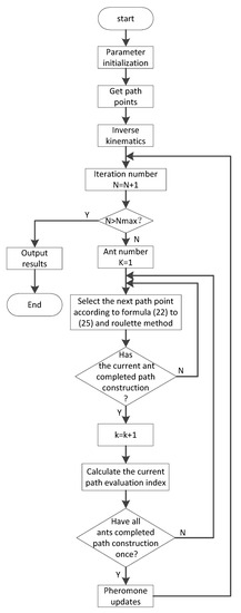
Figure 5.
Overall algorithm flowchart.
The proposed method was compared with the previous methods to demonstrate the proposed method’s superiority. The proposed method differs from previous methods in the following two aspects:
(1) The proposed method uses a point cloud simplification method based on a continuous grid partition. Laser processing is characterised by a variable laser spot size. The grid sizes are computed using a recursive method, which can work well with this characteristic. Meanwhile, conventional methods use point cloud slicing technology to obtain regular routes, which means the distance between path points is constant. The proposed method has higher efficiency because a larger spot size can improve efficiency at a position with a small curvature change. (2) The conventional methods’ core idea is to use regular curves or broken lines to traverse the fixed area without considering many optimisation conditions. The proposed method uses an improved ant colony algorithm for path planning so that different optimisation conditions can be considered and better solutions can be obtained than traditional methods.
5.2. Standard Test
To demonstrate the performance of the improved algorithm, the algorithm was compared with two classical ACO (MMAS and ACO) algorithms.
For the TSP benchmark EIL51 from TSPLIB, every algorithm was executed 100 times, and all distances, including those from each point to all other points, were defined to be integers in the experiment.
Table 3 presents the statistical results of the three algorithms. Figure 6 depicts the change in the cost function value in each iteration. The x-axis indicates the number of iterations, and the y-axis represents the route distance of the three algorithms. As the data were selected from the best iteration, Figure 6 also depicts the shortest iteration number of the three algorithms.
Table 3.
Comparison of IMMAS with other ant colony algorithms.
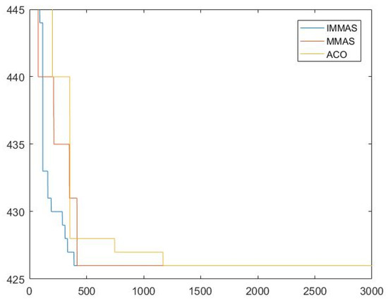
Figure 6.
Route distance comparisons per each iteration from the best iteration of each algorithm.
IMMAS exhibited a better performance, although all three algorithms found the optimal solution in the eil51 problem. With regard to global search ability, IMMAS exhibited a better performance in terms of average path length, maximum path length, and standard deviation of path length in the eil51 problem. The shortest number of iterations of IMMAS was also the smallest. Therefore, IMMAS is valid and can obtain a better solution, with a quality better than that of the other algorithms.
5.3. Application Test
To verify the feasibility and effect of the method proposed, it was tested using a manipulator, as depicted in Figure 7. This manipulator was a 6-DOF serial manipulator equipped with a scanner and laser generator to process the sample piece depicted in Figure 2.
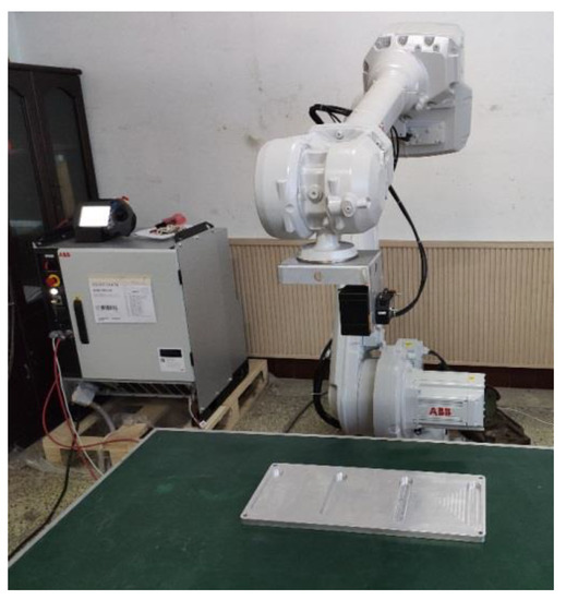
Figure 7.
Experimental scene picture.
The processing method used in this test was laser processing. Laser processing is characterised by a variable laser spot size. In combination with this characteristic, the method introduced in Section 2 significantly simplifies the point cloud model. Figure 8 depicts the path generated by the proposed method.
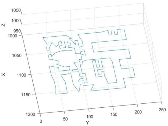
Figure 8.
Path generated by the method proposed in this paper.
Then, the point cloud slicing technology was applied. This method cuts the point cloud model through a series of parallel planes at an equal interval. To ensure the processing accuracy at each point, the point cloud model is divided at small intervals. Figure 9 depicts the path generated by the point cloud slicing technology.
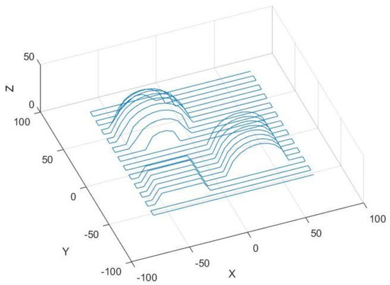
Figure 9.
Path generated by the point cloud slicing technology.
Table 4 presents the results of the two methods. The proposed method obtained better performance and generated a more efficient path. The optimisation value is calculated using the model described in Section 3, according to Equation (12).
Table 4.
Comparison of the two methods.
To specify the utility of the proposed approach in terms of real-world sensing applications, it was used for laser cleaning of rust on the steel surface. Figure 10 depicts the effect of laser cleaning. Most of the rust has been removed with the proposed method for path planning.
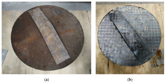
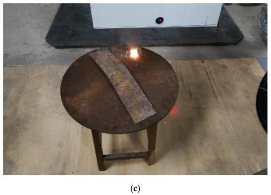
Figure 10.
Effect of laser cleaning: (a) workpiece before cleaning, (b) workpiece after cleaning, and (c) workpiece during cleaning.
6. Conclusions and Further Studies
The coverage path generation in a complex free-form surface is a representative problem that has been steadily investigated in path planning and automatic control. Most methods, including the point cloud slicing method, use regular curves or broken lines to traverse the fixed area. The drawback is that they need to be improved in terms of efficiency and effect.
To overcome these issues, the path-planning method was divided into three parts: environmental modelling, optimisation objectives and boundary conditions, and optimisation methods. New methods were used in each part.
(1) Laser processing is characterised by a variable laser spot size. A new point cloud processing algorithm was proposed for environmental modelling, which can work well with this characteristic.
(2) For optimisation objectives, a novel path evaluation model was established by introducing the trajectory optimisation information. For different task objects and task demands, more types of path shape can be obtained by adjusting the weight coefficients’ concrete value and normalisation coefficients.
(3) An improved ant colony algorithm was proposed to solve the CPP problem. Based on the max–min ant system, two improvement measures were proposed. One was a method of calculating the transition probability based on randomness. The other was the addition of a relative factor in the process of pheromone updating. The numerical studies indicated that the improvement measures improved the global search ability of the algorithm, and the improved ant colony algorithm obtained better performance than that of ACO and MMAS.
Combining all three parts, a new CPP method was proposed based on point cloud data. The test results revealed that the method generated a more efficient path than the point cloud slicing technology that is currently commonly used. Thus, the proposed method provides a useful reference for the path planning of manipulators on complex free-form surfaces. However, due to the heuristic algorithm’s randomness, the global optimal solution cannot be obtained each time. Besides, some of the optimisation target parameters also need to be modified after experimental verification, which increases the complexity of using the proposed method for different tasks. More-effective metaheuristic algorithms and path evaluation models should be considered to achieve much quicker and more-practical coverage path generation in further studies. Moreover, the ant colony algorithm should be combined with the commonly used parallelism framework to improve the algorithm’s running speed, thus reducing the proposed method’s overall running time.
Author Contributions
Conceptualisation, Y.D. and L.L.; methodology, X.Y. and Y.W.; software, X.Y. and L.L.; supervision, L.H.; writing—original draft, X.Y.; writing—review and editing, L.H. All authors have read and agreed to the published version of the manuscript.
Funding
This research was funded by the National Natural Science Foundation of China, grant number 5187052280, and the Sichuan Action and Innovation Driven Fund Project of “Made in China 2025”.
Conflicts of Interest
The authors declare no conflict of interest.
References
- Yang, G.W. Laser ablation in liquids: Applications in the synthesis of nanocrystals. Prog. Mater. Sci. 2007, 52, 648–698. [Google Scholar] [CrossRef]
- Simakin, A.V.; Obraztsova, E.D.; Shafeev, G.A. Laser-induced carbon deposition from supercritical benzene. Chem. Phys. Lett. 2000, 332, 231–235. [Google Scholar] [CrossRef]
- Bonse, J.; Krueger, J.; Hoehm, S.; Rosenfeld, A. Femtosecond laser-induced periodic surface structures. J. Laser Appl. 2012, 24, 042006. [Google Scholar] [CrossRef]
- Lei, Z.; Tian, Z.; Chen, Y. Laser Cleaning Technology in Industrial Fields. Laser Optoelectron. Prog. 2018, 55, 030005. [Google Scholar]
- Santos, L.C.; Santos, F.N.; Solteiro Pires, E.J.; Valente, A.; Costa, P.; Magalhaes, S. Path Planning for ground robots in agriculture: A short review. In Proceedings of the 2020 IEEE International Conference on Autonomous Robot Systems and Competitions (ICARSC), Ponta Delgada, Portugal, 15–17 April 2020; pp. 61–66. [Google Scholar]
- Zafar, M.N.; Mohanta, J.C. Methodology for Path Planning and Optimization of Mobile Robots: A Review. In Proceedings of the 1st International Conference on Robotics and Smart Manufacturing (RoSMa), Chennai, India, 19–21 July 2018; pp. 141–152. [Google Scholar]
- Patle, B.K.; Babu, G.L.; Pandey, A.; Parhi, D.R.K.; Jagadeesh, A. A review: On path planning strategies for navigation of mobile robot. Def. Technol. 2019, 15, 582–606. [Google Scholar] [CrossRef]
- Choset, H. Coverage for robotics—A survey of recent results. Ann. Math. Artif. Intel. 2001, 31, 113–126. [Google Scholar] [CrossRef]
- Chen, C.H.; Song, K.T. Complete coverage motion control of a cleaning robot using infrared sensors. In Proceedings of the IEEE International Conference on Mechatronics (ICM), Taipei, Taiwan, 10–12 July 2005; IEEE: Piscataway, NJ, USA, 2005; pp. 543–548. [Google Scholar]
- Bosse, M.; Nourani-Vatani, N.; Roberts, J. Coverage algorithms for an underactuated car-like vehicle in an uncertain environment. In Proceedings of the IEEE International Conference on Robotics and Automation, Rome, Italy, 10–14 April 2007; IEEE: Piscataway, NJ, USA, 2007; pp. 698–703. [Google Scholar]
- Yordanova, V.; Gips, B. Coverage Path Planning With Track Spacing Adaptation for Autonomous Underwater Vehicles. IEEE Robot. Autom. Lett. 2020, 5, 4774–4780. [Google Scholar] [CrossRef]
- Majeed, A.; Lee, S. A New Coverage Flight Path Planning Algorithm Based on Footprint Sweep Fitting for Unmanned Aerial Vehicle Navigation in Urban Environments. Appl. Sci. 2019, 9, 1470. [Google Scholar] [CrossRef]
- Dakulovic, M.; Petrovic, I. Complete coverage path planning of mobile robots for humanitarian demining. Ind. Robot 2012, 39, 484–493. [Google Scholar] [CrossRef]
- Galceran, E.; Carreras, M. A survey on coverage path planning for robotics. Robot. Auton. Syst. 2013, 61, 1258–1276. [Google Scholar] [CrossRef]
- Hong, L.; Jiayao, M.; Weibo, H. Sensor-based complete coverage path planning in dynamic environment for cleaning robot. Caai Trans. Intell. Technol. 2018, 3, 65–72. [Google Scholar]
- Khan, A.; Noreen, I.; Habib, Z. On Complete Coverage Path Planning Algorithms for Non-holonomic Mobile Robots: Survey and Challenges. J. Inf. Sci. Eng. 2017, 33, 101–121. [Google Scholar]
- Choset, H. Coverage of Known Spaces: The Boustrophedon Cellular Decomposition. Auton. Robot. 2000, 9, 247–253. [Google Scholar] [CrossRef]
- Yang, S.X.; Luo, C.M. A neural network approach to complete coverage path planning. IEEE Trans. Syst. Man Cybern. Part B Cybern. 2004, 34, 718–725. [Google Scholar] [CrossRef]
- Gabriely, Y.; Rimon, E. Spanning-tree based coverage of continuous areas by a mobile robot. Ann. Math. Artif. Intel. 2001, 31, 77–98. [Google Scholar] [CrossRef]
- Ishida, S.; Rigter, M.; Hawes, N. Robot Path Planning for Multiple Target Regions. In Proceedings of the 2019 European Conference on Mobile Robots (ECMR), Prague, Czech Republic, 4–6 September 2019; p. 6. [Google Scholar]
- Morin, M.; Abi-Zeid, I.; Petillot, Y.; Quimper, C.G. A Hybrid Algorithm for Coverage Path Planning With Imperfect Sensors. In Proceedings of the IEEE International Conference on Intelligent Robots and Systems, Tokyo, Japan, 3–7 November 2013; Amato, N., Ed.; IEEE: Piscataway, NJ, USA, 2013; pp. 5988–5993. [Google Scholar]
- Shivgan, R.; Ziqian, D. Energy-Efficient Drone Coverage Path Planning using Genetic Algorithm. In Proceedings of the 2020 IEEE 21st International Conference on High Performance Switching and Routing (HPSR), Newark, NJ, USA, 11–14 May 2020; p. 6. [Google Scholar]
- Jin, J.; Tang, L. Optimal Coverage Path Planning for Arable Farming on 2d Surfaces. Trans. ASABE 2010, 53, 283–295. [Google Scholar] [CrossRef]
- Lee, T.; Baek, S.; Choi, Y.; Oh, S. Smooth coverage path planning and control of mobile robots based on high-resolution grid map representation. Robot. Auton. Syst. 2011, 59, 801–812. [Google Scholar] [CrossRef]
- Noreen, I.; Khan, A.; Habib, Z. A Review of Path Smoothness Approaches for Non-holonomic Mobile Robots. In Proceedings of the 2018 Computing Conference, London, UK, 10–12 July 2019; pp. 346–358. [Google Scholar]
- Xie, J.; Carrillo, L.R.G.; Jin, L. Path Planning for UAV to Cover Multiple Separated Convex Polygonal Regions. IEEE Access 2020, 8, 51770–51785. [Google Scholar] [CrossRef]
- Modares, J.; Ghanei, F.; Mastronarde, N.; Dantu, K. UB-ANC planner: Energy efficient coverage path planning with multiple drones. In Proceedings of the 2017 IEEE International Conference on Robotics and Automation (ICRA), Singapore, 29 May–3 June 2017; IEEE: Piscataway, NJ, USA, 2017; pp. 6182–6189. [Google Scholar]
- Alexa, M.; Behr, J.; Cohen-Or, D.; Fleishman, S.; Levin, D.; Silva, C.T. Computing and rendering point set surfaces. IEEE Trans. Vis. Comput. Graph. 2003, 9, 3–15. [Google Scholar] [CrossRef]
- Lin, A.C.; Liu, H.T. Automatic generation of NC cutter path from massive data points. Comput. Aided Des. 1998, 30, 77–90. [Google Scholar] [CrossRef]
- Zhen, X.; Seng, J.; Somani, N. Adaptive Automatic Robot Tool Path Generation Based on Point Cloud Projection Algorithm. In Proceedings of the 24th IEEE International Conference on Emerging Technologies and Factory Automation (ETFA), Zaragoza, Spain, 10–13 September 2019; IEEE: Piscataway, NJ, USA, 2019; pp. 341–347. [Google Scholar]
- Zou, Q.; Zhao, J. Iso-parametric tool-path planning for point clouds. Comput. Aided Des. 2013, 45, 1459–1468. [Google Scholar] [CrossRef]
- Masood, A.; Siddiqui, R.; Pinto, M.; Rehman, H.; Khan, M.A. Tool Path Generation, for Complex Surface Machining, Using Point Cloud Data. Procedia CIRP 2015, 26, 397–402. [Google Scholar] [CrossRef]
- Lian, Q.; Li, X.; Li, D.; Gu, H.; Bian, W.; He, X. Path planning method based on discontinuous grid partition algorithm of point cloud for in situ printing. Rapid Prototyp. J. 2019, 25, 602–613. [Google Scholar] [CrossRef]
- Zhang, H.; Li, L.; Zhao, J. Robot automation grinding process for nuclear reactor coolant pump based on reverse engineering. Int. J. Adv. Manuf. Tech. 2019, 102, 879–891. [Google Scholar] [CrossRef]
- Chen, W.; Li, X.; Ge, H.; Wang, L.; Zhang, Y. Trajectory Planning for Spray Painting Robot Based on Point Cloud Slicing Technique. Electronics 2020, 9, 908. [Google Scholar] [CrossRef]
- Zhang, G.F.; Wang, J.W.; Cao, F.; Li, Y.; Chen, X.Q. 3D Curvature Grinding Path Planning Based on Point Cloud Data. In Proceedings of the 12th IEEE/ASME International Conference on Mechatronic and Embedded Systems and Applications (MESA), Auckland, New Zealand, 29–31 August 2016; IEEE: Piscataway, NJ, USA, 2016. [Google Scholar]
- Verscheure, D.; Demeulenaere, B.; Swevers, J.; De Schutter, J.; Diehl, M. Time-Optimal Path Tracking for Robots: A Convex Optimization Approach. IEEE Trans. Autom. Contr. 2009, 54, 2318–2327. [Google Scholar] [CrossRef]
- Gregory, J.; Olivares, A.; Staffetti, E. Energy-optimal trajectory planning for robot manipulators with holonomic constraints. Syst Control. Lett. 2012, 61, 279–291. [Google Scholar] [CrossRef]
- Piazzi, A.; Visioli, A. Global minimum-jerk trajectory planning of robot manipulators. IEEE Trans. Ind. Electron. 2000, 47, 140–149. [Google Scholar] [CrossRef]
- Constantinescu, D.; Croft, E.A. Smooth and time-optimal trajectory planning for industrial manipulators along specified path. J. Robot. Syst. 2000, 17, 233–249. [Google Scholar] [CrossRef]
- Huang, J.; Hu, P.; Wu, K.; Zeng, M. Optimal time-jerk trajectory planning for industrial robots. Mech. Mach. Theory 2018, 121, 530–544. [Google Scholar] [CrossRef]
- Duan, H.; Zhang, R.; Yu, F.; Gao, J.; Chen, Y. Optimal Trajectory Planning for Glass-Handing Robot Based on Execution Time Acceleration and Jerk. J. Robot. 2016, 2016, 1–9. [Google Scholar] [CrossRef]
- Dorigo, M.; Maniezzo, V.; Colorni, A. Ant system: Optimization by a colony of cooperating agents. IEEE Trans. Syst. Man Cybern. Part B Cybern. 1996, 26, 29–41. [Google Scholar] [CrossRef] [PubMed]
- Stutzle, T.; Hoos, H.H. MAX-MIN Ant System. Future Gener. Comp. Syst. 2000, 16, 889–914. [Google Scholar] [CrossRef]
- Mahi, M.; Baykan, O.K.; Kodaz, H. A new hybrid method based on Particle Swarm Optimization, Ant Colony Optimization and 3-Opt algorithms for Traveling Salesman Problem. Appl. Soft Comput. 2015, 30, 484–490. [Google Scholar] [CrossRef]
- Blum, C.; Puchinger, J.; Raidl, G.R.; Roli, A. Hybrid metaheuristics in combinatorial optimization: A survey. Appl. Soft Comput. 2011, 11, 4135–4151. [Google Scholar] [CrossRef]
- Deng, W.; Xu, J.; Zhao, H. An Improved Ant Colony Optimization Algorithm Based on Hybrid Strategies for Scheduling Problem. IEEE Access 2019, 7, 20281–20292. [Google Scholar] [CrossRef]


Publisher’s Note: MDPI stays neutral with regard to jurisdictional claims in published maps and institutional affiliations. |
© 2020 by the authors. Licensee MDPI, Basel, Switzerland. This article is an open access article distributed under the terms and conditions of the Creative Commons Attribution (CC BY) license (http://creativecommons.org/licenses/by/4.0/).