Abstract
The article aims to prove the hypothesis, that an approach direction influences repeatability at target point of a trajectory. Unlike most researches that deal with absolute accuracy, this paper is focused on determining the achievable repeatability and the influence of the direction of approach on it. To prove the hypothesis, several measurements are performed under different conditions, on industrial robot ABB IRB1200. To verify and confirm the result obtained from the resolvers located on the individual axes of the robot, the measurements are replicated using high-speed digital image correlation cameras. Using an external measuring device, the real repeatability of the robot endpoint is determined. The measurement proved the correctness of the hypothesis, i.e., the dependence of the approach direction on repeatability was proved. Furthermore, real deviations were measured and the extent of this influence on the robot repeatability was determined.
1. Introduction
Industrial robots and manipulators are generally considered to be universal systems that can be operated in any industrial conditions, in any way. However, the purpose of the manipulator is given by the mounted tool—its installation considerably limits the versatility of the manipulator. In industrial conditions, it is the rule that the manipulator is a part of a single-purpose machine, production line, or other equipment. In these cases, it is usually possible to operate only in a specific way, usually performing one specific task cyclically. Therefore, in cases where it is necessary to increase the precision of the manipulator, it may be not necessary to increase the absolute accuracy in the entire working envelope of the robot, but it might be sufficient to increase repeatability only for specific targets.
In terms of industrial manipulator precision, two different values are generally addressed—accuracy and repeatability. Accuracy is the ability of the robot to reach a tool center points (TCPs) programmed pose with respect to the robot´s base frame. Repeatability is ability of the robot to return its TCP (tool center point) to the same position, repeatedly from the same direction.
The accuracy of the manipulator is affected by several external influences. In addition to temperature, manufacturing inaccuracies, shaft deflection and clearances in bearings and gearboxes, it can be, for example, the fact that the resolvers (or encoders) are located at the beginning of the drive unit, and therefore, do not detect an error that occurs on the motor and gearbox [1]. Repeatability is caused by clearances, resolution of position sensors, thermal expansion, and other influences. It does not include the coordinate system setting errors, other than the modelled arm length, manufacturing, and assembly deviations (e.g., non-perpendicularity or non-parallelism of joints and guides).
While absolute accuracy can vary by up to 15 mm [2] compared to the ideal model in the case of large manipulators, and it is necessary to use an external device, such as a laser tracker for measuring and increasing accuracy, repeatability is usually in the range of tenths to hundredths of a mm [1]. However, it depends on the operating conditions a lot. The values given by the manufacturer usually apply to a steady state under ideal conditions and for a new manipulator. Nevertheless, there are applications in which an ordinary level of repeatability may not appear to be sufficient, especially for less rigid robot structures.
For example, ABB offers the Absolute Accuracy and CalibWare Option for its robots [2]. This functionality aims to eliminate the difference between an ideal manipulator in a Computer-aided design (CAD) environment and the real robot installed on a factory site. The correction solves not only the mechanical properties and inaccuracies of the particular manipulator but also deviations caused by an inaccurately defined payload. An advantage is also the interchangeability of the robot “piece by piece” if necessary, as the accuracy of robots, calibrated by this method, is consistent. The difference between an ideal virtual and a real manipulator is usually in the range of 8–15 mm, depending on the type of robot and the concurrence of manufacturing tolerances and deviations. This technique uses a laser tracker to measure accuracy at one hundred targets within the entire robot workspace, based on this measurement, calibration within the entire robot working envelope is provided. The resulting accuracy is generally 0.5 mm, but typically not lower [2].
Calibration methods based on the use of a laser tracker [3,4] are commonly used in industrial applications. Further research in this field focuses for example on an additional increase of accuracy of this method by making a big number of measurements (in the order of tens of thousands) as described in [5]. This is achieved by a measuring system that communicates with the robot controller and the laser tracker, while the robot configurations are chosen with the help of a deep neural network. Laser trackers are often used as a reference measurement to evaluate the properties of other calibration methods [6,7,8,9]. Another use of lasers for robot calibration is in the form of laser interferometry-based sensing and measurement as described in [10]—this method provides real-time dynamic position measurements with high accuracy, high sampling rate, and large working space. A 3D measurement system consisting of a commercially available telescoping ball bar system is proposed in [9]. After calibrating the robot in selected 72 poses of the end-effector with respect to the base, verification in 10,000 random robot configurations made by comparison with a laser tracker confirmed approximately two times better accuracy of the robot than before the calibration. A geometric method of calibration is also described in [11] with a special focus on finding the best calibration poses of the robot to achieve the highest possible improvement in positioning accuracy. The authors in [12] point out a problem that applies to all calibration methods and is related to the influence of backlash of the robot joints. This effect is described in the article together with a proposed method for the elimination of this source of additional error. A commonly used group of methods for robot calibration is based on photogrammetry. One of the approaches is to use a 3D photogrammetry-based measuring device to track the position and orientation of the robot end-point in real-time and use this information as feedback for the robot controller [13]. Photogrammetry is also applied in off-line robot calibration [6]. Research has also been done in the area of use of a commercially-available portable photogrammetry system in industrial robot calibration, the authors in [7] compare this approach with a laser tracking calibration with very good results—the accuracy of photogrammetry is only slightly worse. The research in [14] describes the use of a camera mounted on the robot end-effector and a calibration board placed in the workplace where the camera can see it most of the time. This proposed calibration method also works on-line. A similar solution with a single camera mounted near the robot end-point was introduced also in [15] and the achieved improvement in robot accuracy was between three to six times. As far as high-speed cameras are concerned, authors in [16] utilized the Phantom v2511 camera with up to 25,000 frames per second to ascertain the accuracy of an industrial robot not only in the absolute value but also concerning the movement direction. Such a system can also be used to measure dynamic movement, oscillation, vibration, etc. Application of stereo-vision for robot calibration has also been the subject of research, for example in [17] a method for increasing the accuracy of an industrial milling robot with the help of a stereo camera is described. In addition, another research was done using low-cost systems [18] or laser-camera-triangulation [19].
Unlike photogrammetry, the digital image correlation method enables full-field 3D displacement measurements, allowing the correlation system to be used in both vibration analysis and deformation analysis of components. The main advantage over point measurement is the possibility of including more data in the processing of results. Since the measurement is carried out on a surface, in addition to position information, it is also possible to obtain information about the direction of the surface normal. If the high-speed cameras are used, it is possible to analyze kinematics, dynamics, and vibration of the manipulator in detail, or to measure its modal properties. The study in [20] describes a motion analysis of a two-arm service robot as it passes between two positions. It was a large-scale application designed to reconstruct the movement of the manipulator in space. The measurement results were 3D trajectories of three joint nodes and vibration responses in these nodes during robot movement. The authors in [21] proposed an algorithm of simple iterative learning control of a robot, whose aim was to reduce geometric errors occurring in the technology process known as single point incremental sheet forming. They apply the 3D digital image correlation method to measure the geometric error along the tool path. In addition to position measurement, the DIC method can also be used in operational vibration analysis or experimental modal analysis. Several papers have been published on this topic [22,23,24,25,26,27]. In the paper [26], the authors proposed a highly efficient procedure for processing large amounts of data representing the vibration time responses of the analyzed structure. This procedure was subsequently implemented in the DICMAN 3D software application for modal test evaluation. In another work [27], the authors went even further by presenting a technique that makes it possible to use a DIC system to measure vibration responses during body movement. It is based on post-processing numerical elimination of the rigid body motion components. They used this technique to measure the modal shapes and operating shapes of the rotating disk. These approaches can be advantageously used in the analysis of dynamic behavior of robots and manipulators, e.g., to reduce dynamic load when accelerating, decelerating, or optimizing trajectory.
Most of the scientific publications are focused on measurement and increase of the robot absolute accuracy. According to the aim of this article, it is also necessary to mention those that address the measurement of repeatability.
A team of researchers from the University of Žilina described a methodology of pose-repeatability measurement, based on the use of laser interferometer and digital indicator [28]. This paper uses the recommended procedure described in the ISO 9283:1998—international standard that describes how performance characteristics should be specified [29]. Experimental measurement of robot repeatability is also described in a paper from Robert Morris University, USA [30].
We must not forget to mention articles focused on a comparative evaluation of industrial robots using different types of methods [31,32,33].
It is clear from the above overview that the area of increasing the accuracy or repeatability of manipulators is an area, that has long been paid attention to, and several possible solutions have been presented to increase the precision. However, none of these methods examines in more depth the influence of arrival direction at the desired target.
The paper aims to prove the dependence of the arrival direction to the target on repeatability and to determine the range of directional deviation for a specific robot by a set of measurements.
2. Conditions and Procedure for Hypothesis Verification
- According to the authors’ assumption, there is a dependence between the direction of the robot arrival at the target and the repeatability that can be achieved at this target. Based on the summary stated above, the authors claim that this influence is not considered in the case of robot repeatability increasing attempts done by other researchers.
- In the first phase, only robot drives resolver data will be used for verification. These data should already prove the dependence of the direction of approach on the repeatability of the robot in the measured target. For this reason, the joint variables will be converted (according to the forward kinematics task) to the endpoint deviation (x, y, z, and the total deviation). Since the data from the revolvers do not include the error that occurs in the gearbox, arm deflection, thermal expansion, and also does not include the influence of manufacturing tolerances and deviations of individual parts of the manipulator mechanical structure, the second phase of measurement will follow.
- In the next phase, the target position and orientation will be measured by the 3D DIC method, and the deviation in the repeatability spectrum will be evaluated with high precision.
- As a result of the measurement, there will be a graphical representation of the measured target vicinity and the degree of deviation valid for its directions of approach.
- The result of this experimental measurement will be valid for a specific industrial robot, with a defined solution of installation in the workplace and for a specific target.
3. Description of the Measured Robot
The ABB IRB1200 5/0.9 industrial robot was chosen for the experiments. It is a compact angular six-axis robot with IP40 protection, which is designed for work in clean indoor spaces, for applications such as packaging, handling, assembly, etc.
According to the manufacturer, the repeatability of the manipulator is 0.025 mm and the robot can be set in any orientation at any angle. Table 1 contains the basic technical parameters of the robot. The forward reach of the robot is 901 mm with a load capacity of 5 kg (with the center of gravity at a maximum distance of 100 mm from the flange).

Table 1.
Basic parameters of IRB1200 5/0.9 [1].
The experiments are performed at the workstation with a pair of the ABB IRB1200 robots—the robots are mounted on a pedestal so that the bases of the robots are not in a horizontal position but are inclined by an angle of 40° in the y-axis of the coordinate system of each of the robots. This is not a standard mounting position of the robot, in this case, the first axis of the robot is loaded by torque even if it maintains a position (any other than 0°) or rotates at a constant speed. This fact directly affects the accuracy and repeatability of the robot.
The robot was warmed-up before every measurement and kept at a constant temperature as much as possible. This is a standard routine for every precise robot programming task. Before the robot targets are precisely calibrated, the robot is kept in the movement for some time, to warm up its structure in a way it will be warmed during its production
For measurement, the robot is equipped with payloads of various parameters (Figure 1, Table 2), which simulates real operating conditions, where robots rarely carry minimal mass. There is a black-and-white speckle pattern for subsequent verification of repeatability by the DIC method glued on the front surface of the payload.
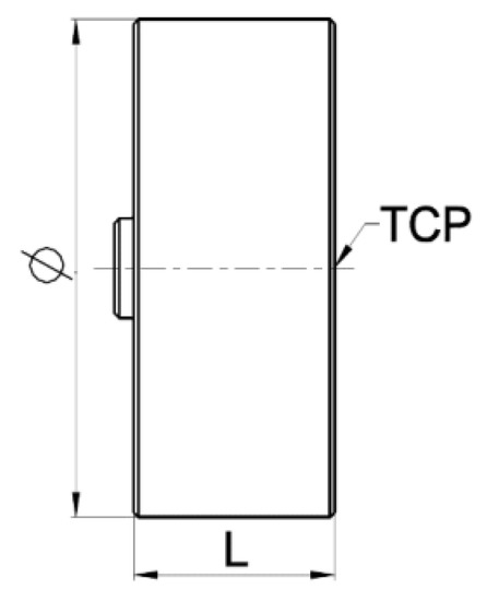
Figure 1.
Payload side view.
Table 2.
Payload parameters.
4. The Experiment
This chapter describes the first phase of measurement, which aims to prove the influence between the robot approach direction to the end target and the repeatability that can be achieved at this target.
Before starting the experiment, it was necessary to determine the minimal oscillation stabilization time when the robot is stopped. The stabilization time was chosen based on the results of the dynamic measurement of the robot arm stabilization during its sudden stop/start. The necessary data were obtained from three-axis accelerometers applied in two places—directly on the effector (on the side of the analyzed payload—see Figure 2) and the base of the robot. A typical effector oscillation recorded in one of the accelerometer axes is shown in Figure 3. Although in this case, the arm can be considered stabilized after approximately 0.6 s, for a higher degree of certainty in the measurement the time for stabilization was tripled.
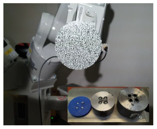
Figure 2.
Robot payload with applied black-and-white speckle pattern.
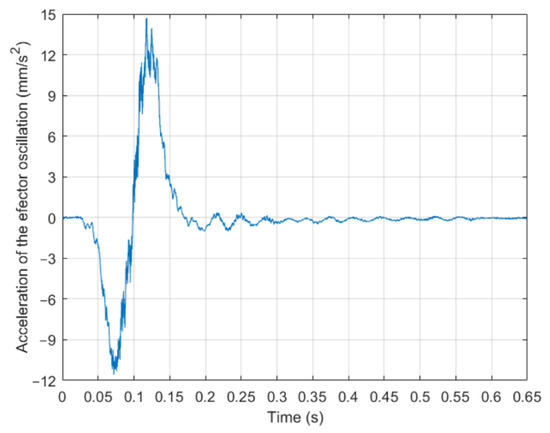
Figure 3.
The stabilization process of the robot effector, recorded after a stop at the target point.
The flowchart in Figure 4 describes the experiment process. The ABB IRB 1200 robot equipped with a cylindrical payload whose TCP lies at the intersection of the front plane of the cylinder and its axis of symmetry cycles continuously to the same point, but from different directions (from different starting points). The movement definition is entered parametrically into the control application (written in C #), which runs on a computer and collects data from the robot. The parameters of the robot during the measurement are contained in Table 3.
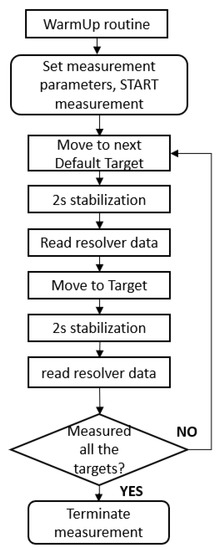
Figure 4.
Experiment control system flowchart.
Table 3.
Robot measurement movement parameters.
All starting positions within one cycle are located at the same distance from the measured target—the default positions form a spherical surface created according to the specified diameter and density using the principle of spherical Fibonacci lattice [34]. The coordinates (x, y, z) are updated by the control application and correspond to points on the spherical surface with the defined diameter. The orientation at the default positions is not changed. Due to the orientation of the manipulator, only the front hemisphere is considered.
The spherical Fibonacci lattice is used as the simplest solution for the even distribution of the defined number of points on a spherical surface. Points are distributed evenly regardless of the diameter. By the even distribution, it is meant that the distance between every two adjacent points is the same.
The precise description for every single default position is not necessary, the result should be the suitability of arrival from all the directions to the destination target, shown by a gradient between multiple points. From such a graph, it will be possible to determine relatively accurate values for the error caused by the direction of approach to a point, anywhere in the hemisphere, i.e., even around precisely specified points (Figure 5).
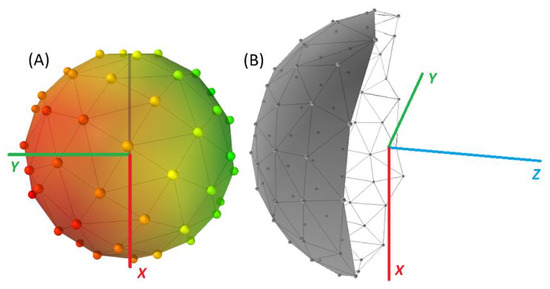
Figure 5.
(A): Points, evenly distributed on the spherical surface. (B): Semi-sphere with origin orientation.
A total of 24 cycles were performed with different values of the radius of the mentioned sphere (50, 100, 150, 200, 250, 300 mm), the number of starting positions (10, 20, 40, 80, 160), and the number of repetitions (10, 20, 30). All combinations of the parameters of performed measurements are listed in Table 4, Table 5, Table 6, Table 7 and Table 8. Visualization of the location of the hemisphere is shown in Figure 6. The measured target has the same orientation as the TCP (tool coordinate system), and is located at the distance of +500 mm in the direction of WCS (world coordinate system) axis. The WCS is shown in Figure 6 on the left. The position and orientation of the TCP (tool coordinate system) are displayed on the robot tool. In the middle of Figure 6 is the hemisphere, along its surface, the default positions are evenly distributed.
Table 4.
Parameters for measurements of the influence of the number of repetitions.
Table 5.
Parameters for measurements of the influence of the number of starting positions.
Table 6.
Parameters for measurements of the influence of the radius dimension.
Table 7.
Parameters for measurements of the influence of the payload.
Table 8.
Parameters for measurements of the influence of the measured target position.
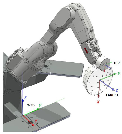
Figure 6.
Robot workspace and measured target.
5. Experimental Results
To confirm the hypothesis that the endpoint repeatability depends, among other things, on the direction of approach to this point, it was necessary to realize the selected measurements in three different ways. For each of these measurements, a set of starting points was created, then three different measurements were executed under the same conditions, with the difference that in the first measurement the points were selected in order from the lowest to the highest value of the y-axis (yMIN → yMAX), the second measurement was in the opposite direction (yMAX → yMIN) and in the third one, the points were chosen in random order.
The joint variables (j1—j6 (°)) were always read and then the values for the same points were compared when measuring in a different overall order.
From the graphs (Figure 7) it is evident that the deviation depends only on the position of the starting point relative to the endpoint. Whether these starting points for the approach are selected in order from one side or the other one, or completely randomly, is not important. This result, among other things, excludes accidental errors or other influences that would cause randomness in these results.
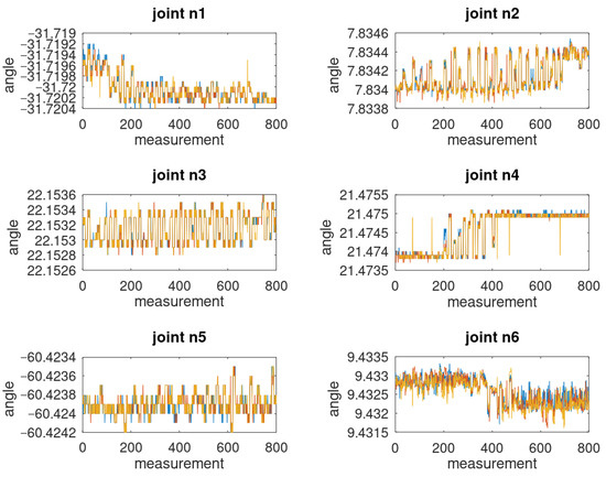
Figure 7.
Deviations of joints (°) in the ordered and random selection of default positions.
The waveforms of individual measurements almost completely overlap with only a minimal difference between the first “yellow” measurement (yMIN → yMAX), in which the points were executed from the lowest y-axis value to highest. Red (yMAX → yMIN), was executed in the opposite order and blue using a completely random order of points. All three waveforms have been sorted from YMIN to YMAX, due to the possibility of comparing the same points in these measurements.
According to the mathematical model, the position and deviations of the tool center point can be calculated based on the forward kinematics task, but this value varies in the spectrum of absolute inaccuracy.
To determine the repeatability and the real deviations from the selected target, it is necessary to measure the precision at the endpoint (TCP). For this purpose, the 3D DIC methodology will be applied in the second phase, to verify the results.
Individual measurements are also shown in the form of box-plot graphs, its principle is described in Figure 8. Symbols represent values outside the basic range (outliers). If the value is greater than three times the quartile, it is displayed with the symbol “o”, the symbol “+” is used to display the value in the range 1.5–3 [35].
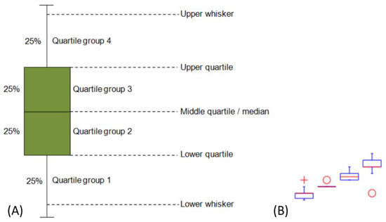
Figure 8.
(A): Quantile of measured values [36]. (B): Symbols displaying values outside the basic range.
The graphs below (Figure 9 and Figure 10) show the influence of the approach direction on the individual joint variables of the robot. As already mentioned in the article, these data come from the drive resolvers of the individual axis of the robot, i.e., they do not include errors that occur “higher” on the structure.
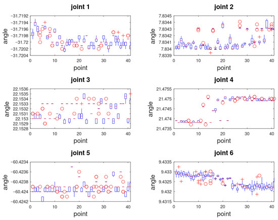
Figure 9.
Error (°) distribution on individual robot joints during Measurement 14.
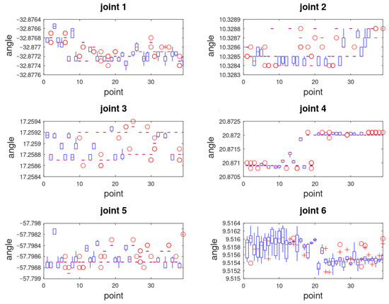
Figure 10.
Error (°) distribution on individual robot joints during Measurement 16.
The figures (Figure 9 and Figure 10) show data from robot drive resolvers—the results of Measurements 14 and 16 according to tables (Table 6 and Table 7). All the realized measurements were evaluated in this way. However, to better understand the facts found, and especially to determine the real precision of the manipulator, it is necessary to convert these data to repeatability values on the endpoint of the robot, i.e., the TCP point (see Figure 11). This recalculation is realized by the generally known methodology of the forward kinematics task, the Denavit–Hartenberg parameters used for this recalculation are described in Table 9 below.
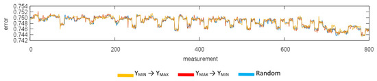
Figure 11.
Deviations (mm) in the gradual and random selection of default positions, display for the robot flange (tool center point—TCP).
Table 9.
D-H parameters of ABB IRB 1200 5/0.9 [1].
Figure 11 below displays the overall deviations of the TCP, calculated from given D-H parameters. Three measurements are shown and the idea is the same as in Figure 7, i.e., to prove that the deviation is affected by the direction of approach to the measured target. In Figure 11, all three waveforms have been sorted from YMIN to YMAX, due to getting a comparison of the same points.
Selected measurements, converted to the TCP deviation, are described by the figures below (Figure 12 and Figure 13).
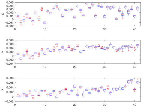
Figure 12.
Error (mm) distribution on the TCP during Measurement 14.
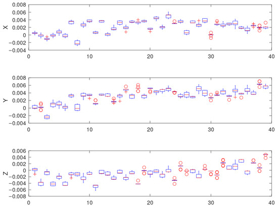
Figure 13.
Error (mm) distribution on the TCP during Measurement 16.
The representation of the results in the form of a 3D map (Figure 14) may seem to be clearer. It is obvious at first glance which directions of approach to the measured target are and are not suitable from the repeatability point of view. The color gradient shows the measured repeatability error corresponding to the respective starting point. The orientation of view to the surface of the hemisphere is always in the direction of the positive x-axis, i.e., towards the measuring device. Deviations in the x, y, and z axes were measured, as well as the resulting normal and total error. The resulting deviation is usually the result of the average of ten measurements. From the figures below (Figure 14) it is apparent that under the conditions defined in Measurements 14 and 16, the most convenient direction of approach is from the target´s y-axis direction. The higher values of the deviation in Figure 14 are caused by a robot control system, which predicts that the mechanical structure will bound by this value. However, this prediction leaves an opportunity for further repeatability increase. The points in the graphs (Figure 12 and Figure 13) are sorted from YMIN to YMAX values, i.e., from the bottom of the semi-sphere to its top.
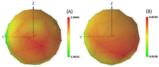
Figure 14.
(A): Distribution of the total error (mm) in Measurement 14. (B): Distribution of the total error (mm) in Measurement 16.
6. Verification of the Results and Determination of Real TCP Deviations Using DIC
The measurements described above (Table 4, Table 5, Table 6, Table 7 and Table 8) were also performed to focus the end part of the robot, i.e., the front side of the cylindrical payload. The aim was to verify the results obtained from robot resolvers, and especially to determine the real deviation of TCP in the spectrum of repeatability, i.e., including clearances in the gearboxes of individual axes of the robot, the effect of thermal expansion, arm deflection, manufacturing inaccuracies, etc.
The Dantec Dynamics Q-450 high-speed digital image correlation system was used for this purpose (Figure 15). This 3D measuring system consists of two high-speed digital cameras SpeedSense 9070 with 16 GB of memory and CMOS sensors enabling recording in max. HD resolution (1280 × 800 px) up to a frame rate of 3140 FPS. The cameras are connected to a laptop with the Istra4D control software. Thanks to the large dynamic measuring range, the device allows recording movements in the range from a few micrometers up to tens of centimeters, during which it uniquely combines high image resolution with highly accurate time resolution. Other technical parameters of the Q-450 correlation system are given in Table 10.
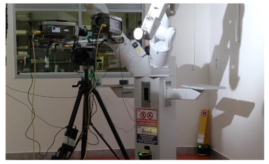
Figure 15.
Measurement of IRB1200 by DIC Q-450 system.
Table 10.
Technical parameters of the Q-450 Dantec Dynamics system.
The above-mentioned measuring system works on the principle of digital image correlation, i.e., comparison of digital images recorded during the experiment. Image correlation is performed on small image elements called facets. It is usually a group of square pixels with a size from 15 × 15 px to 30 × 30 px, but depending on the type of the task, the size of the facet can be adjusted (reduced or enlarged). For a correct image correlation, it is important to ensure that each facet is unique, i.e., it contains a unique pixel distribution with different levels of grey color intensity. Therefore, a random black-and-white pattern is formed on the surface of the analyzed object. The facets may touch or overlap, but there may not be an empty area between them. Since the information about the displacements of the analyzed object is obtained at the nodes of the virtual grid, which correspond in position to the centers of the facets, the overlap of the facets (Figure 16) is one way to increase the image resolution, i.e., to obtain a larger amount of data and thus to better reconstruct the surface (especially around the edges) of the analyzed object. The manufacturer of correlation devices Dantec Dynamics recommends overlapping the facets up to 1/3 of the size of the facet because, with such an overlap, the data points are still independent.
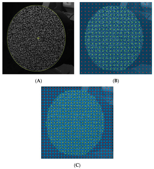
Figure 16.
Illustrative example of the increase of the image resolution caused by the facet overlap: (A): defined area of interest, (B): measuring points when the facets are in touch, (C): measuring points when the facets are overlapped.
The calibration process, leading to the assessment of the internal and external calibration parameters of the cameras, is performed by the automatic acquisition of the calibration target in many different positions. The calibration of Q-450 Dantec Dynamics cameras is based on Zhang’s algorithm. After calibration, the position of the 3D point (in camera coordinates) is transformed into the sensor coordinates (see Figure 17). The coordination transformation process is described in detail in [37].
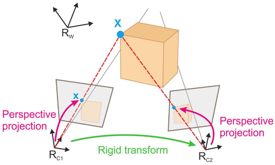
Figure 17.
The scheme of the transformation of the analyzed point world coordinates into the sensor coordinates.
To obtain information about the transformation coordinates of the points of the analyzed object, Dantec Dynamics correlation devices use an algorithm based on a pseudo-affine transformation [38]. If the transformation parameters of possible displacement, elongation, shear, and distortion of the facet a0–a7 (Figure 18) are considered, according to the above-mentioned algorithm the transformation coordinates (u, v) can be calculated as follows:
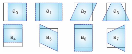
Figure 18.
Transformation parameters used in the algorithm based on a pseudo-affine transformation.
The measurement procedure was the same as in the case of robot joint variables measurement. The flowchart (Figure 4) was only extended (Figure 19) as follows (three images are always taken):
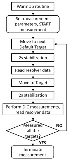
Figure 19.
Flowchart of the experiment control system (DIC).
To determine the effect of robot drift, Measurement 4 (Table 1, Figure 20) was performed. Drift can seriously affect the repeatability and accuracy if the robot structure temperature changes significantly. The drift could be prevented by keeping the structure at the optimal working temperature (by cooling in with fans in foundry applications, for example). Measurement 4 results however, proved, that for conditions under which all the measurements took place, the influence of drift is not significant. The pre-warm-up routine was used before every measurement to get the system to its optimal operating temperature.
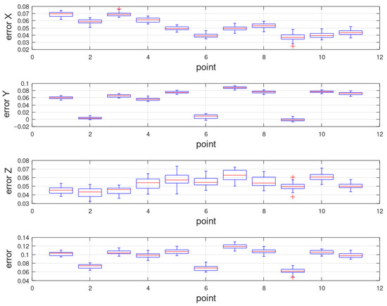
Figure 20.
Manipulator repeatability (mm), Measurement 4.
According to the “3D Map (Figure 21) it is evident, that at a given position of the point relative to the robot, the repeatability can be increased simply by changing the direction of approach to the target Figure 21 shows Measurements 14 and 16 (radius 250/300 mm, 40 different default positions, different carried weight) displaying its total errors. The points are sorted from YMIN to YMAX i.e., from the bottom of the semi-sphere to its top.
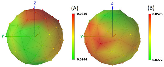
Figure 21.
(A): Total error (mm), Measurement 14. (B): Total error (mm), Measurement 16.
From the figures, it is apparent that under the defined conditions, the most convenient direction of approach is from the VII octant for Measurement 14 and the top (z-axis) in case of Measurement 16.
For the selected measurements, the real repeatability values (mm) measured by DIC are displayed in Figure 22 and Figure 23. From the Measurement 14 results (Figure 22), it is evident that the carried weight influences the repeatability predominantly in the middle sections (mid-range of point’s y value) of error graphs. In the case of Measurement 16 (Figure 23), the difference in repeatability values within the measured hemisphere is not significant.
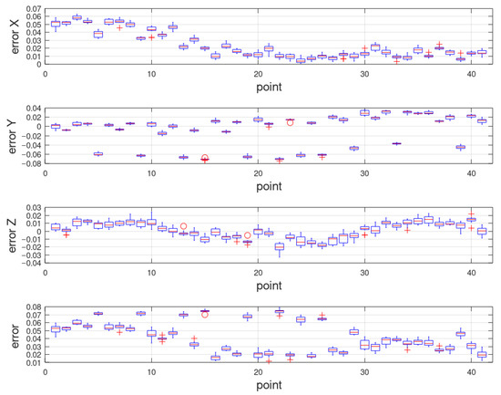
Figure 22.
Manipulator repeatability (mm), Measurement 14.
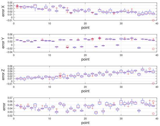
Figure 23.
Manipulator repeatability (mm), Measurement 16.
Measurements 20 and 21 (Figure 24, Figure 25 and Figure 26) were performed under the same conditions, in different measured targets (see Table 8). As these two measured targets are not too far apart and robot axis orientation was not too different, there is only a slight difference between these two results. However, the difference between the most convenient/least suitable direction of arrival is almost 0.09 mm for Measurement 20 (0.07 mm in Measurement 21) and so this could be the repeatability increase if the approach trajectory will be changed according to the information from the graphs.
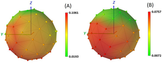
Figure 24.
(A): Total error (mm), Measurement 20. (B): Total error (mm), Measurement 21.
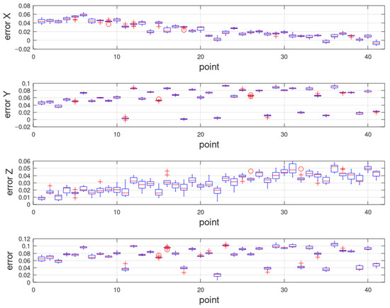
Figure 25.
Manipulator repeatability (mm), Measurement 20.
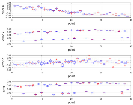
Figure 26.
Manipulator repeatability (mm), Measurement 21.
7. Conclusions
The hypothesis that the repeatability of the robot at the target depends, among other things, on the direction of approach to it, has been proven.
The graphs (Figure 7 and Figure 11) show that the error does not occur randomly (the deviation of the approach to the target was the same regardless of the order in which the starting points were evaluated). By recalculating the results of the measured values of the joint variables to the positioning deviation of the tool center point, the repeatability was determined (inaccuracies that belong to the individual directions of approach at the target).
Many influences affect the repeatability value. Especially the thermal expansion will always affect any high-precision device. For this reason, the robot was warmed-up before every measurement and kept at a constant temperature as much as possible.
The data given by the resolvers cannot be used to determine the most accurate direction for an approach to a target. It is caused by the fact, that in these data, the arm and shaft deflection is not contained. Resolver data have been used only to prove the hypothesis. The real accurate data could be given only by the external measurement device, DIC in this case.
To verify the ascertainment and especially to obtain real and accurate values of robot repeatability, all measurements were replicated with the use of the 3D DIC methodology. The results of these measurements are displayed not only in the form of box-plot graphs but also in 3D maps, that better illustrate the achieved results.
The dependence of the direction of approach on the repeatability, achievable at the target, was verified at several points. In Measurements 19–24, the target point was shifted by 150 mm in both directions of all the world coordinate system axes. The hypothesis was, therefore, verified not only under different parameters of the robot’s movement but also at seven different targets.
The degree of this dependence varies with respect to other parameters, such as the weight carried or the approach speed. For example, in Measurement 20 (Figure 24 and Figure 25), the difference from the (zero, exact) value is +0.019 (max) and +0.106 (min). If, for example, depending on the nature of the process and the workplace, it is possible to approach from the most advantageous direction, there may be a refinement compared to the least advantageous direction, by 0.087 mm in the order of the total deviation of repeatable accuracy.
This research presents a new opportunity to increase the repeatability of any robotic arm. According to the knowledge of the surrounding space and its influence on the tool center point deviation, the trajectory could be slightly changed or improved so that the repeatability will be increased. Authors in this research used the DIC cameras to measure the real state, but any external device, which is accurate enough would be used.
The provided measurement is not permanent, regular calibration will be required as in any other accurate device.
In a practical application, a high precision assembly task, for example, the procedure would be as follows:
- Prepare the robot and external technologies to an operational state;
- Set DIC cameras, define a control application inputs (orientation of measured target, number of points on sphere, number of repetitions from every single initial point, etc.);
- Run the robot’s movement to the measured target, measure the reached position by DIC;
- Evaluate the sphere, create the “3D map”, place it into a figure of workstation, to get an orientation of sphere according to the surrounding installation;
- With the information of the most and least suitable approaches of direction, re-program the robot motion to get the better repeatability.
8. Future work
The authors plan to use the described precision measurement methodology to measure the precision of the robot’s movement along the trajectory. After determining the inaccuracies, it will certainly be possible to compensate for these, but the question is to what extent it will be possible to optimize the movement along the trajectory.
Author Contributions
M.V.: Software, writing—review and editing, investigation R.H.: methodology, validation M.H.: software, investigation V.K.: conceptualization, writing—original draft, resources, funding acquisition, T.K.: software, writing—review and editing, visualization Z.B.: methodology, supervision, data curation, formal analysis, validation, project administration. All authors have read and agreed to the published version of the manuscript.
Funding
This work was supported by the European Regional Development Fund in the Research Centre of Advanced Mechatronic Systems Project, project number CZ.02.1.01/0.0/0.0/16_019/0000867 within the Operational Programme Research, Development and Education and project supported by the Scientific grant agency of the Ministry of Education, Science, Research and Sport of the Slovak Republic and the Slovak Academy of Sciences, project number VEGA 1/0355/18: the use of experimental methods of mechanics for refinement and verification of numerical models of mechanical systems with a focus on composite materials.
Conflicts of Interest
The authors declare no conflict of interest.
References
- Technical Data for the IRB 1200 Industrial Robot. Available online: https://new.abb.com/products/robotics/industrial-robots/irb-1200/irb-1200-data (accessed on 26 November 2019).
- ABB Absolute Accuracy: CAlibWare; ABB Inc.: Auburn Hills, MI, USA, 2005; Available online: https://library.e.abb.com/public/0f879113235a0e1dc1257b130056d133/Absolute%20Accuracy%20EN_R4%20US%2002_05.pdf (accessed on 27 November 2019).
- Marek, P.; Piszczek, Ł. Testing of an industrial robot’s accuracy and repeatability in off and online environment. Eksploat. Niezawodn. Maint. Reliab. 2018, 20, 455–464. [Google Scholar] [CrossRef]
- Albert, N.; Bonev, I. Absolute calibration of an ABB IRB 1600 robot using a laser tracker. Robot. Comput. Manuf. 2013, 29, 236–245. [Google Scholar] [CrossRef]
- Gang, Z.; Zhang, P.; Ma, G.; Xiao, W. System identification of the nonlinear residual errors of an industrial robot using massive measurements. Robot. Comput. Manuf. 2019, 59, 104–114. [Google Scholar] [CrossRef]
- Hothmer, J. International archives of photogrammetry and remote sensing. ISPRS J. Photogramm. Remote Sens. 1989, 44, 192. [Google Scholar] [CrossRef]
- Filion, A.; Joubair, A.; Tahan, A.S.; Bonev, I.A. Robot calibration using a portable photogrammetry system. Robot. Comput. Manuf. 2018, 49, 77–87. [Google Scholar] [CrossRef]
- Alici, G.; Shirinzadeh, B. A systematic technique to estimate positioning errors for robot accuracy improvement using laser interferometry based sensing. Mech. Mach. Theory 2005, 40, 879–906. [Google Scholar] [CrossRef]
- Nubiola, A.; Bonev, I. Absolute robot calibration with a single telescoping ballbar. Precis. Eng. 2014, 38, 472–480. [Google Scholar] [CrossRef]
- Shirinzadeh, B.; Teoh, P.; Tian, Y.; Dalvand, M.M.; Zhong, Y.; Liaw, H. Laser interferometry-based guidance methodology for high precision positioning of mechanisms and robots. Robot. Comput. Manuf. 2010, 26, 74–82. [Google Scholar] [CrossRef]
- Wu, Y.; Klimchik, A.; Caro, S.; Furet, B.; Pashkevich, A. Geometric calibration of industrial robots using enhanced partial pose measurements and design of experiments. Robot. Comput. Integr. Manuf. 2015, 35, 151–168. [Google Scholar] [CrossRef]
- Tian, W.; Liu, W.L.S.; Tian, L.Z.W.; Jiao, J. The problem in Accuracy Compensation of Industrial Robot. Int. Robot. Autom. J. 2017, 3, 1–3. [Google Scholar] [CrossRef]
- Sepehr, G.; Shu, T.; Xie, W.-F.; Joubair, A.; Bonev, I. Accuracy enhancement of industrial robots by on-line pose correction. In Proceedings of the 2017 2nd Asia-Pacific Conference on Intelligent Robot Systems (ACIRS), Wuhan, China, 16–18 June 2017; IEEE: Piscataway, NJ, USA, 2017; pp. 214–220. [Google Scholar] [CrossRef]
- Du, G.; Zhang, P. Online robot calibration based on vision measurement. Robot. Comput. Integr. Manuf. 2013, 29, 484–492. [Google Scholar] [CrossRef]
- Motta, J.M.S.; De Carvalho, G.C.; McMaster, R. Robot calibration using a 3D vision-based measurement system with a single camera. Robot. Comput. Manuf. 2001, 17, 487–497. [Google Scholar] [CrossRef]
- Jerzy, J.; Ostrowski, D.; Jarosz, P.; Mika, D. Industrial robot repeatability testing with high speed camera phantom v2511. Adv. Sci. Technol. Res. J. 2016, 10, 86–96. [Google Scholar] [CrossRef][Green Version]
- Möller, C.; Schmidt, H.C.; Shah, N.H.; Wollnack, J. Enhanced Absolute Accuracy of an Industrial Milling Robot Using Stereo Camera System. Procedia Technol. 2016, 26, 389–398. [Google Scholar] [CrossRef]
- Martin, G.; Joubair, A.; Bonev, I. Local and closed-loop calibration of an industrial serial robot using a new low-cost 3D measuring device. In Proceedings of the 2016 IEEE International Conference on Robotics and Automation (ICRA), Stockholm, Sweden, 16–21 May 2016; IEEE: Piscataway, NJ, USA, 2016; pp. 4312–4319. [Google Scholar] [CrossRef]
- Heiko, K.; Konig, A.; Kleinmann, K.; Weigl-Seitz, A.; Suchy, J. Predictive robotic contour following using laser-camera-triangulation. In Proceedings of the 2011 IEEE/ASME International Conference on Advanced Intelligent Mechatronics (AIM), Budapest, Hungary, 3–7 July 2011; IEEE: Piscataway, NJ, USA, 2011; pp. 422–427. [Google Scholar] [CrossRef]
- Trebuňa, F.; Huňady, R.; Hagara, M.; Virgala, I. High-speed Digital Image Correlation as a Tool for 3D Motion Analysis of Mechanical Systems. Am. J. Mech. Eng. 2015, 3, 195–200. [Google Scholar] [CrossRef]
- Fischer, J.D.; Woodside, M.R.; Gonzalez, M.M.; Lutes, N.A.; Bristow, D.A.; Landers, R.G. Iterative learning control of single point incremental sheet forming process using digital image correlation. Procedia Manuf. 2019, 34, 940–949. [Google Scholar] [CrossRef]
- Wang, W.; Mottershead, J.E.; Ihle, A.; Siebert, T.; Schubach, H.R. Finite element model updating from full-field vibration measurement using digital image correlation. J. Sound Vib. 2011, 330, 1599–1620. [Google Scholar] [CrossRef]
- Results and Experiences from the Application of Digital Image Correlation in Operational Modal Analysis. Acta Polytech. Hung. 2013, 10, 159–174. [CrossRef]
- Reu, P.L.; Rohe, D.P.; Jacobs, L.D. Comparison of DIC and LDV for practical vibration and modal measurements. Mech. Syst. Signal Process. 2017, 86, 2–16. [Google Scholar] [CrossRef]
- Beberniss, T.J.; Ehrhardt, D.A. High-speed 3D digital image correlation vibration measurement: Recent advancements and noted limitations. Mech. Syst. Signal Process. 2017, 86, 35–48. [Google Scholar] [CrossRef]
- Huňady, R.; Hagara, M. A new procedure of modal parameter estimation for high-speed digital image correlation. Mech. Syst. Signal Process. 2017, 93, 66–79. [Google Scholar] [CrossRef]
- Huňady, R.; Pavelka, P.; Lengvarský, P. Vibration and modal analysis of a rotating disc using high-speed 3D digital image correlation. Mech. Syst. Signal Process. 2019, 121, 201–214. [Google Scholar] [CrossRef]
- Kuric, I.; Tlach, V.; Ságová, Z.; Císar, M.; Gritsuk, I. Measurement of industrial robot pose repeatability. MATEC Web Conf. 2018, 244, 01015. [Google Scholar] [CrossRef]
- STN ISO 9283. Manipulating Industrial Robots–Performance Criteria and Related Test Methods; IOS: Geneva, Switzerland, 1995. [Google Scholar]
- Şirinterlikçi, A.; Tiryakioğlu, M.; Bird, A.; Harris, A.; Kweder, K. Repeatability and Accuracy of an Industrial Robot: Laboratory Experience for a Design of Experiments Course. Technol. Interface J. 2009, 9, 53–63. [Google Scholar]
- Nubiola, A.; Slamani, M.; Joubair, A.; Bonev, I. Comparison of two calibration methods for a small industrial robot based on an optical CMM and a laser tracker. Robotica 2014, 32, 447–466. [Google Scholar] [CrossRef]
- Slamani, M.; Joubair, A.; Bonev, I. A comparative evaluation of three industrial robots using three reference measuring techniques. Ind. Robot. Int. J. 2015, 42, 572–585. [Google Scholar] [CrossRef]
- Slamani, M.; Nubiola, A.; Bonev, I.A. Assessment of the positioning performance of an industrial robot. Ind. Robot. Int. J. 2012, 39, 57–68. [Google Scholar] [CrossRef]
- Keinert, B.; Innmann, M.; Sänger, M.; Stamminger, M. Spherical fibonacci mapping. ACM Trans. Graph. 2015, 34, 1–7. [Google Scholar] [CrossRef]
- Octave Forge: Produce A Box Plot. Available online: https://octave.sourceforge.io/statistics/function/boxplot.html (accessed on 21 May 2020).
- Understanding and Interpreting Box Plots: How to Read a Box Plot/Introduction to Box Plots. Available online: https://www.wellbeingatschool.org.nz/information-sheet/understanding-and-interpreting-box-plots. (accessed on 2 June 2020).
- Burger, W. Zhang’s Camera Calibration Algorithm: In-Depth Tutorial and Implementation, Technical Report HGB16-05, University of Applied Sciences Upper Austria, School of Informatics, Communications and Media, Dept. of Digital Media, Hagenberg, Austria. May 2016. Available online: https://www.researchgate.net/publication/303233579_Zhang’s_Camera_Calibration_Algorithm_In-Depth_Tutorial_and_Implementation (accessed on 11 November 2020).
- Trebuňa, F.; Huňady, R.; Hagara, M. Experimental Methods of Mechanics-Digital Image Correlation (In Slovak), 1st ed.; Technical University of Košice: Košice, Slovakia, 2015; pp. 49–50. [Google Scholar]


Publisher’s Note: MDPI stays neutral with regard to jurisdictional claims in published maps and institutional affiliations. |
© 2020 by the authors. Licensee MDPI, Basel, Switzerland. This article is an open access article distributed under the terms and conditions of the Creative Commons Attribution (CC BY) license (http://creativecommons.org/licenses/by/4.0/).