Measurement and Evaluation for Interbedded Pore Water Pressure of Saturated Asphalt Pavement under Vehicle Loading

Featured Application

A closer to actual pavement pore water pressure test method was designed in this study. The empirical formula of pore water pressure as a function of vehicle speed and the Abp empirical formula were obtained by this experimental method.

Abstract

Dynamic water scouring damage is the main cause of pavement structure damage, and the main reason for dynamic water scouring damage is the rapid change of pore water pressure caused by vehicle load. Numerical simulation is a commonly used pore water pressure test technology, but its accuracy is not high, and the test data are very different to actual values. In this study, a pore water pressure test method is designed, which has the advantages of less disturbance to the pavement structure and the measured data are closer to the true pore water pressure value of the pavement structure. Measurement data show that the pore water pressure gradually increases with increasing vehicle speed, and the pore water pressure response time becomes shorter. The pore water pressure response time is greater than vehicle loading time. Moreover, the phenomenon of periodic decay of pore water pressure with time is analyzed based on hydrodynamic water hammer theory. The empirical formula of maximum positive pressure with speed and the empirical formula of Abp at different speeds were obtained.

1. Introduction

Dynamic water scouring damage is a major form of pavement distress that causes government to undergo high maintenance cost [1,2,3]. As the asphalt pavement is a layered structure, pores are easily formed at the joint between layers. In the rainy season, the water in the asphalt pavement repeatedly scours and squeezes the internal structure of the asphalt pavement under the load of the vehicle. The frequent dynamic water scouring and pumping in the pore induces the physical separation of aggregate and asphalt binder film, which causes the loss of strength and stiffness of asphalt mixture [4,5,6,7,8,9].

The pore water pressure evolution of asphalt mixtures under vehicle loading was also evaluated by various researchers: Arambula et al. developed a simple experimental procedure to measure the water vapor diffusion coefficients in coarse aggregates, fine aggregate mixtures, and hot-mixed asphalt, and the numerical simulation of the instantaneous diffusion of moisture in the cross-section microstructure of the asphalt mixture analysis. The results show that the water diffusion coefficient of the asphalt mixture itself directly affects the degree of water damage [10]. Khalili et al. presented the partial differential equations governing non-isothermal flow and deformation in an elastic medium with double porosity [11]. Kettil et al. simulated the water flow induced by the moving wheel pressure on wet asphalt road pavements, which may be a reason for a damage phenomenon in asphalt denoted stripping [12]. Cai et al. utilized Biot’s fully dynamic poroelastic theory to account for the coupling between the soil skeleton and pore water in the medium [13]. Gao et al. designed a fiber optic dynamic hydraulic pressure sensor (FODHPS) based on the principle of fiber Bragg grating (FGG) sensing, and the dynamic water pressure of road surface was measured based on the instrument by a laboratory test [14].

In summary, there is a unified evaluation index and a perfect evaluation system for asphalt pavement water damage under the action of static water. However, the research on dynamic water scour damage of pavement structure lacks effective and systematic methods. The numerical simulation of dynamic water pressure is the most used research method at the present stage, and the field measurement of dynamic water pressure is rare and has large defects. Further, there is no industry-accepted experimental method and evaluation standard for evaluating the change of asphalt pavement performance under the action of dynamic water pressure. Therefore, a piezoresistive water pressure sensor is embedded in the Hui-Wu expressway (in Songyuan City, Jilin Province), and the pore water pressure is measured in the field by the sensor. Then, the evolution of pore water pressure under vehicle loading is studied based on a mathematical statistics method.

2. Experimental facility

2.1. Requirements of Sensor

2.1.1. Sensor Frequency Requirements

When the car runs at a speed v on the road, the time that the tire passes through a certain section p of the road surface is t, which is shown in Figure 1. During the time t, the sensor must collect enough data to faithfully reflect the change of pore water pressure.

The grounding dimension of the tire is length × wide = s × b, then the distance traveled by the tire is s, t=s/v.

The ground length of the Volkswagen MAGOTAN tires used in the article is 175.6 mm, and the speed of cars on the highway is generally 40–120 km/h. When the car passes through the interface P at a speed of 120 km/h, the elapsed time is only 5.27 ms. At least five data are needed in the process to reflect the approximate shape of the curve. Then, the sensor is required to have a high frequency. If the frequency of the sensor is 100 Hz, that is to say that 1 ms collects a data, the sensor can acquire 5 data during 5.27 ms.

In conclusion, if the pore water pressure is expected to be recorded when the tire passes through a section at high speed, the acquisition frequency of the sensor should be above 100 Hz.

2.1.2. Sensor Range Requirements

During vehicle loading, there is not only positive pore water pressure in the pavement structure, but also the negative pore water pressure caused by pumping, which requires the sensor to measure both positive and negative pressures.

The accuracy of the sensor is closely related to its measurement range. The larger the measurement range, the greater the measurement error. Thus, the measurement range of the sensor should be slightly larger than the maximum pore water pressure and not too large. A large number of numerical calculations and theoretical analyses have been carried out to calculate the value of pore water pressure [15,16,17]. For example, the pore water pressure of the pavement layers was calculated in the range of 100 kpa to 500 kpa in 2005 by Luo ZG [18]. In 2012, Luo SP calculated that the maximum pore water pressure of the saturated asphalt pavement was 513 kpa [19]. In 2007, Dong ZJ calculated that the maximum dynamic pressure of pavement was about 480 kpa [20]. The review shows that the maximum pore water pressure of saturated asphalt pavement is around 500 kpa. Considering all aspects, the upper limit of the sensor range should be controlled at 500 kpa–1 Mpa, and the lower limit can be 100 kpa.

2.2. Sensor Selection

According to the above analysis, a piezoresistive dynamic water pressure sensor is selected in this paper. The piezoresistive sensor is currently the most widely used sensor, the advantages are listed below.

• Wide frequency response range and high natural frequency.
• Small size. Due to the integrated circuit process, silicon diaphragm sensitive components can be made very small.
• High precision, good sensitivity, suitable for dynamic measurement.
• Because the piezoresistive pressure sensor is integrally formed, it has the advantages of reliable operation, shock resistance, impact resistance, corrosion resistance, and strong anti-interference ability.

The piezoresistive pressure sensor used in this paper has a measurement range of −90 kpa to 700 kpa, an overload accuracy of 0.1%, and a collection frequency of 1000 HZ. The appearance of sensor is a cylinder with a diameter of 2 cm and a height of 6 cm. The upper surface of the cylinder is a hollow cylinder with an outer diameter of 1 cm, an inner diameter of 0.4 cm, and a height of 1 cm. The bottom of the hollow cylinder is a stressed diaphragm with a circle of 0.4 cm and 1 cm from the top surface. As shown in Figure 2. The sensor software smart sensor 4.10 is used for data acquisition and analysis.

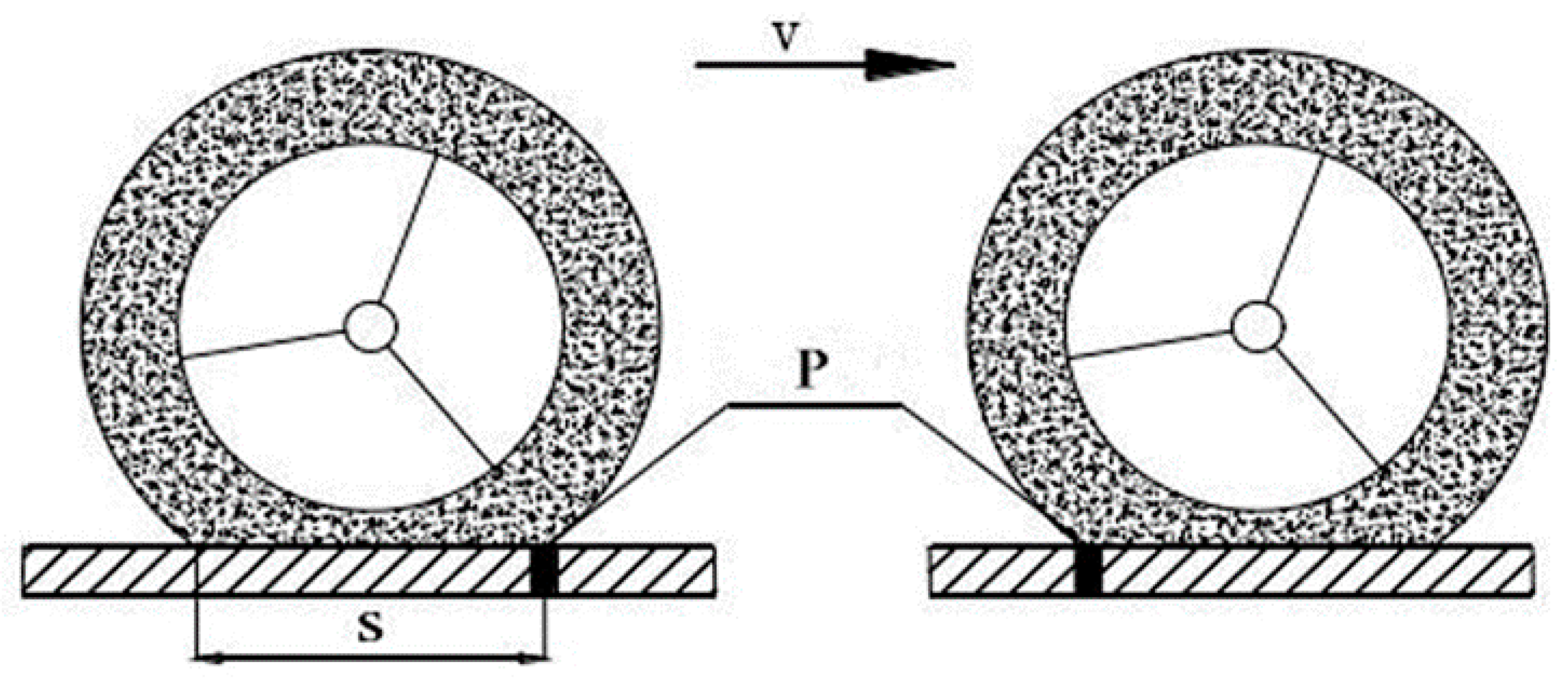
3. Measurement Method Design

3.1. Measurement Method Summary

The main method of the pore water pressure measurement is to directly embed the sensor in the pavement structure. There are two main methods of embedding sensor. Method 1: Post-construction embedding method. Holes are drilled on the already-passed road surface, and the sensors are embedded in holes. This method has good flexibility and can be freely chosen to measure the position. At the same time, it is the most convenient and the easiest to conduct the measurement, but it has the greatest disturbance to the road surface. Method 2: Pre-construction embedding method. In the process of road construction, the sensor is embedded in a predetermined structural layer. The measurement results of this method are closest to the actual situation, and the method has the least disturbance to the pavement structure, but it is the most difficult to achieve. During the roller compaction process, it is difficult to ensure that the sensor is not damaged, but in fact the sensor can be damaged in the process. In addition, during the roller compaction process, the position of the sensor can be changed due to non-uniform force. As a result, the measurement result has a large error.

Therefore, the measurement methods currently used have great problems. Optimizing the measurement method, minimizing the disturbance to the road surface, and preventing the sensor from being damaged are the key problem to be considered in the field measurement of pore water pressure.

3.2. Design of Pore Water Pressure Measurement Method

The measurement location is located on G12 highway in Songyuan City, Jilin Province. The surface structure of G12 highway consists of the lower layer, the middle surface layer and the upper layer. The gradation and thickness of the upper layer are AC-13 and 8 cm, the gradation and thickness of the middle surface layer are AC-20 and 12 cm, the gradation and thickness of the lower layer are AC-25 and 16 cm. According to the structure and the thickness of each layer, a 360 × 360 × 360 mm cube model is prepared and embedded in the pavement to measure the pore water pressure. In the paper, a method for measuring pore water pressure is proposed to solve the above problems.

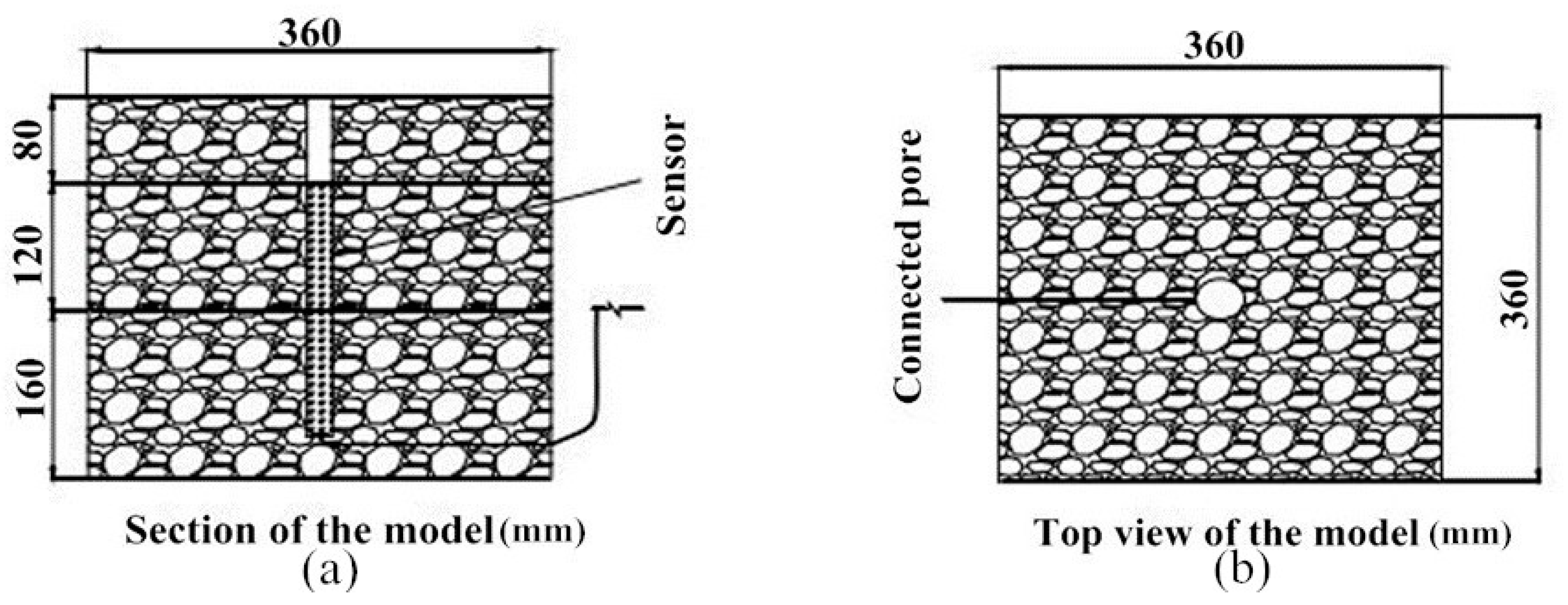
3.2.1. Material Preparation

• According to the gradation and thickness of G12 highway, the plate specimen of the upper layer, the middle surface layer and the lower layer are respectively prepared.
• A connected pore with a diameter of 4 mm that extends vertically through the upper layer are formed at the center of the upper layer by electric drill.
• A vertical hole is drilled in the center of the middle surface layer according to the size of the sensor, so that the sensor can be fixed in the middle surface layer.
• Since the diameter of the data line of the sensor is 8 mm, a vertical hole with a diameter of 10 mm is drilled in the center of the lower layer to ensure the data line can pass through.
• The basic asphalt used in this study is 70# asphalt, which is called “Pan Jin” base asphalt. The basic indicators of the basic asphalt used in this study are summarized in

  Table 1. Basic asphalt of technical indicators.

  Penetration (0.1 mm)	25 °C Ductility (cm)	Softening Point (°C)	Flash Point (°C)	Density (g·cm−3)
  15 °C 25 °C 30 °C
  24.7 61.9 106.9	>100	48.7	260	1.003
  GB/T0606- 2011	GB/T0605- 2011	GB/T0606- 2011	GB/T0611- 2011	GB/T0603- 2011

  .
• The road performance of the asphalt mixture used in this study is shown in

  Table 2. Asphalt mixture road performance.

  High Temperature Performance		Low Temperature Performance		Water Stable Performance
  Marshall stability (KN)	Dynamic stability (times/mm)	Splitting strength (MPa)	Flexural tensile strength (MPa)	Residual stability of immersed Marshall (%)	Residual Marshall stability after 10 days of freezing and thawing (%)
  8.53	3261	3.79	7.51	78.7	81.3

  .

3.2.2. Model Assembly

• The sensor is placed in the hole of the middle surface layer, and the upper surface of the sensor is kept on the same level as the upper surface of the middle surface layer. The upper surface of the sensor is sealed with tape and 150 °C asphalt binder is poured into the gap between the sensor and the hole until the gap is filled. Then the middle surface layer and the sensor are cooled to the normal temperature so that the sensor can be firmly fixed in the middle surface layer.
• A high-strength fine mesh should be covered on the surface of the sensor to prevent the fine particles from clogging the sensor and affecting the measurement result during the measurement process. Considering that the fine mesh should not only prevent the particles from blocking the sensor, but also not affect the pore water pressure, the pore diameter of fine mesh is selected to be 0.2 mm. Remove the adhesive tape stuck on the sensor surface, and carefully clean the upper surface of the sensor, then cover the surface of the sensor with a fine mesh of appropriate size and press the surrounding of the fine mesh into the asphalt binder into the asphalt binder for fixation.
• After the asphalt binder in the middle surface layer is cooled, the data line is passed through the hole in the lower layer. Here, asphalt binder with 150 °C is evenly applied to the lower surface of the middle surface layer and the upper surface of the lower layer, then the middle surface layer and lower layer are glued together to ensure the central axis of the two is in a straight line. After the asphalt binder is cooled and the two are integrated, the gap between the data line and the hole of the lower layer is filled with asphalt binder according to the above steps.
• After 150 °C asphalt binder is evenly applied to the upper surface of the middle surface layer and the lower surface of the upper layer, then the middle surface layer and upper layer are glued together to ensure the central axis of the connected pore in upper layer and the force diaphragm of the sensor in the middle surface layer are on a straight line. Moreover, the connected pore of the upper layer is covered with a fine mesh to prevent fine particles from blocking the connected pore. The model is prepared after it is kept at 15 °C for 3 days.

3.2.3. Model Embedment

• Communicate with the relevant departments and block the single traffic on the road section.
• The rectangular hole with the same size of the model was dug out on the pavement with asphalt concrete cutting machine, and enough gaps are left for the data line to lead out.
• The sidewalls and the bottom of the hole and the sidewall of the model are heated using a blast burner, then the model is hung into the hole and the data line is drawn along the bottom of the model to the road surface. Then, 150 °C asphalt binder is poured into the gap between the side wall of the model and the side wall of the hole until the gap is filled.
• Lead the data line to the workstation on the roadside, and cut out a slot with width and depth of 1 mm through which the data line passes. Put the data line into the slot and fix the data line in the slot with tape to ensure the vehicle will not damage the data line when it passes by. The model embedding work has been completed, as is shown in Figure 3 and Figure 4.

4. Results and Analysis

The measurement is conducted in rainy weather. When the thickness of the water film on the surface of the model is maintained at 5~10 mm, the model is kept under the condition for 1 h. First connect the sensor with the laptop, and then open the software smart sensor 4.10 to verify that the connection is unblocked and set the initial parameters. The weight of the test vehicle is 1600 kg and the pore water pressure is recorded when the vehicle passes through the measurement point at the speed of 20 km/h, 40 km/h, 60 km/h and 80 km/h, respectively. In order to eliminate the influence of errors, parallel experiments were used, repeatedly collecting multiple sets of data, and using the coefficient of variation to eliminate unreasonable data to ensure that the errors in this study are within a reasonable range. The variation of pore water pressure with time at different speeds is shown in Figure 5.

As can be seen from the Figure 5, the pore water pressure increases with the increase of speed, and the pore water pressure decays periodically over time, this phenomenon can be explained by Hydrodynamic water hammer theory [21].

As is shown in Figure 6, when the vehicle load acts on the pores, part of the pore water obtains the initial velocity v, and the flow hits the bottom of the pore and the velocity of the flow at the bottom becomes zero instantaneously, the water pressure at the bottom of the pore increases from ρgh to ρgh + Δp, and a compression wave is formed at the liquid interface between ρgh and ρgh + Δp. This article assumes that the compression wave moves Δs within Δt.

After the compression wave reaches the bottom, the momentum equation of the water flow is described by the Equations (1) and (2).

$$\rho \Delta sA\left(0-v\right)=\left[P-\left(P+\Delta P\right)\right]\Delta t$$

(1)

$$\Delta P=\rho v\frac{\Delta s}{\Delta t}=\rho vc$$

(2)

where c is the speed of the compression wave, v is the initial velocity of the flow under the vehicle load, $\rho$ is the density of water, and A is the cross-sectional area of the pore. When the water pressure at the bottom of the pore increases from ρgh to ρgh + Δp, the density of water and the cross-sectional area of the pores will change. The density of water increases by Δρ, and the cross-sectional area of the pores increase by ΔA. The mass of flow in the ΔS section increases due to the effect of cross-section expansion and water compression, and the added mass is the mass of free water which is replenished from the upper part. According to the law of conservation of mass, Equation (3) can be acquired.

$$\rho vA\Delta t=\left(\rho +\Delta \rho \right)\left(A+\Delta A\right)\left(c\Delta t\right)-\rho A\left(c\Delta t\right)$$

(3)

Simplify and omit higher order infinitesimals to get the following Equation (4).

$$\rho vA=c\left(\rho \Delta A+A\Delta \rho \right)$$

(4)

Then, Equation (5) can be acquired.

$$v=c\left(\frac{\rho \Delta A+A\Delta \rho }{\rho A}\right)=c\left(\frac{\Delta A}{\rho A}+\frac{\Delta \rho }{\rho }\right)$$

(5)

Let $\left(\frac{\Delta A}{\rho A}+\frac{\Delta \rho }{\rho }\right)$ be $\Delta P$. The K bulk modulus of water is equal to the ratio of stress to strain. The Equation (6) can be acquired.

$$K=\frac{\Delta P}{\frac{\Delta v}{v}}=\frac{\Delta P}{\frac{\Delta \rho }{\rho }}$$

(6)

Then, Equation (7) can be acquired.

$$\frac{\Delta \rho }{\rho }=\frac{\Delta P}{K}$$

(7)

Since the diameter of the cylindrical pore is 2 r, Equation (8) can be obtained.

$$\Delta A=\pi \left[{\left(r+\Delta r\right)}^2-r^2\right]=2\pi r\Delta r+\pi \Delta r^2$$

(8)

Omit higher order infinitesimals, Equation (9) can be obtained.

$$\frac{\Delta A}{A}=\frac{2\Delta r}{r}$$

(9)

The E elastic modulus of solids is equal to the ratio of stress to strain. Equation (10) can be acquired.

$$E=\frac{\Delta \sigma }{\frac{\Delta r}{r}}$$

(10)

Then, Equation (11) can be obtained.

$$\frac{\Delta r}{r}=\frac{\Delta \sigma }{E}$$

(11)

According to fluid mechanics, when the balance fluid acts on the pipe wall, the stress generated by the pipe wall is $\Delta \mathsf{\sigma }=\frac{\Delta Pr}{\xi }$. Then, Equation (12) can be obtained.

$$\frac{\Delta r}{r}=\frac{\Delta Pr}{E\xi }$$

(12)

Then, Equation (13) can be obtained.

$$\frac{\Delta A}{A}=\frac{\Delta Pr}{E\xi }$$

(13)

Substituting Equations (13) and (7) into Equation (5), Equation (14) can be obtained.

$$v=c\left(\frac{\Delta P2r}{E\xi }+\frac{\Delta P}{K}\right)=\frac{c\Delta P}{K}\left(1+\frac{2Kr}{E\xi }\right)$$

(14)

Added the static water pressure at the bottom of the pore, the total pore water pressure under vehicle load is shown in Equation (15).

$$P=\frac{Kv}{c\left(1+\frac{2Kr}{E\xi }\right)}+\rho gh$$

(15)

where K is the bulk modulus of water, E is the elastic model of the asphalt mixture, $\rho$ is the density of the water, r is the radius of the cylindrical pore and $\xi$ refers to the range of water pressure on the side wall after the water pressure increases in the pores.

According to the above calculation, when $0<t<h/c$, the compression wave propagates upward from the bottom of the pore. In an ideal situation, the velocity of the water flow at the point where the compression wave is reduced to zero, and the water pressure increases by $\Delta P$. When $t=h/c$, the compression wave reaches the upper surface of the pore, the velocity of the whole water in the pore is reduced to zero and the water pressure at the bottom of the pore becomes maximum at $P=\frac{Kv}{c\left(1+\frac{2Kr}{E\xi }\right)}+\rho gh$. However, there is a pressure difference between the upper and lower ends of the wave at the upper surface of the pore, and the pressurized water in the pore moves upward at the velocity v. At the time, an expansion wave is formed in the pore. When $h/c<t<2h/c$, the expansion wave propagates from top to bottom, the pressure of the water flow at the point where the expansion wave is reduced by Δp, and the water flow moves upward at the velocity v. When $t=2h/c$, the compression wave reaches the bottom of the pore, the whole free water in the pore finish the state of compression and the water pressure at the bottom of pore recovers to $\rho gh$. At this time, the water flow is like a spring under pressure. After the external force is removed, the spring will not only return to its original length, but will also stretch because of inertia. Similarly, the water flow will continue to move upwards at the speed v due to inertia. Therefore, after the compression state is over, the water flow will not be stabilized in the static pressure state, but will be over-expanded and the pressure of water flow will continue to decrease. Until the pressure of water flow drops to $-\Delta P$, the water at the bottom of the pore is stable, which in turn produces a new expansion wave. When $2h/c<t<3h/c$, the new expansion wave propagates from bottom to top, the pressure of the water flow at the point where the new expansion wave reaches is reduced by Δp, and the water flow at the point where the new expansion wave not reaches still moves upward at velocity v. When $t=3h/c$, the new expansion wave reaches the upper surface of the pore. At this time, the water pressure at the bottom of the pore becomes $-\left(\frac{Kv}{c\left(1+\frac{2Kr}{E\xi }\right)}-\rho gh\right)$, and the pressure difference between the upper and lower ends of the wave is $\Delta P-\rho gh$, thus a new compression wave is generated in the pore. When $3h/c<t<4h/c$, the new compression wave propagates from top to bottom, the pressure of the water flow at the point where the compression wave reaches recovers to P, the water flow moves down at the velocity v. When $t=4h/c$, the new compression wave reaches the upper surface of the pore, and the water flow still moves towards the bottom of the pore at the velocity v. Then, the pore water pressure circulates periodically, and the pore water pressure cycle is $t=4h/c$.

The above analysis is based on the assumption that the energy of the water flow in the pores is conserved, the pores are not connected with other pores, the permeability of the asphalt concrete material is zero, and there is no energy loss in the process. However, the actual situation is not the case. The asphalt concrete has permeability, and it will contract and deform under load, and the pores in the pavement structure are not regular shapes. Therefore, the pore water pressure in the pavement decays periodically over time. In addition, the reversal from positive to negative pore water pressure should be an important inducement for the loss of adhesion between asphalt and aggregate.

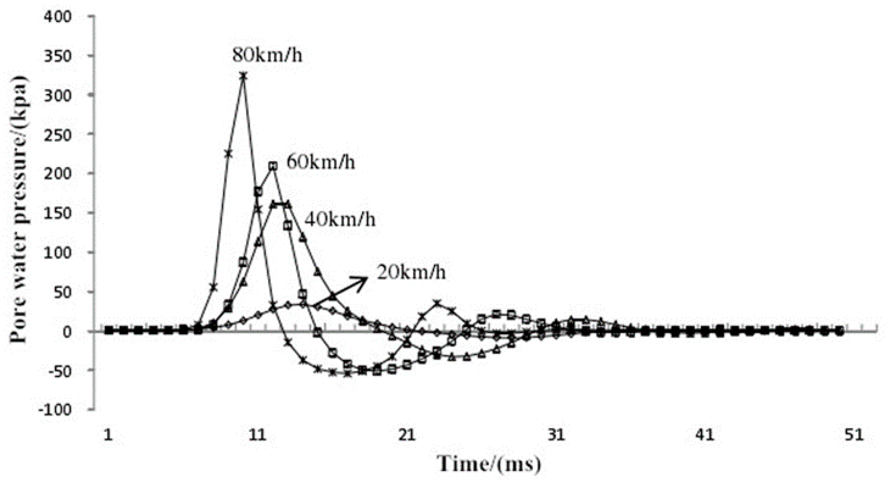
4.1. Analysis of Relationship between Pore Water Pressure and Vehicle Speed

The peak pore water pressure at different speed is shown in

Table 3. The peak pore water pressure at different speed.

Vehicle Speed (km/h)	Maximum Positive Pressure (kpa)	Maximum Negative Pressure (kpa)
20	34.003	−8.589
40	161.351	−32.747
60	209.692	−51.094
80	324.245	−53.714

.

It can be seen from the table that the maximum negative pressure is only 1/4 to 1/6 of the maximum positive pressure, which means that the damage effect of pumping on the asphalt pavement is weak during the whole process of dynamic water scouring damage. The maximum positive pressure increases with the increase of vehicle speed, and the empirical formula of maximum positive pressure with speed is calculated by Equation (16).

$$\mathrm{y}=0.2472x^{1.6671}$$

(16)

where y is the maximum positive pressure, and x is the vehicle speed, and the correlation coefficient of the regression equation is 0.9826.

As can be seen from Figure 5, there are two obvious cycles in the pore water pressure response curve at different vehicle speeds. Take the pore water pressure response curve at 20 km/h speed as an example, the start time of the first cycle is 4 ms, the end time is 35 ms, and the cycle is 31 ms; the start time of the second cycle is 35 ms, the end time is 53 ms, and the cycle is 18 ms. After two cycles, the pore water pressure is maintained at a static water pressure of between 0.7 and 1 kpa. The peaks and troughs of pore water pressure response curve in two cycles are listed in the

Table 4. The peaks and troughs of pore water pressure response curve in two cycles at 20 km/h.

Cycle	The First Cycle		The Second Cycle
Response time (ms)	10	24	33	40
Peaks and troughs (kpa)	34.00	−8.59	1.94	−0.04

.

The absolute values of peak and trough of pore water pressure response curve (Abp) at different time are plotted in the Figure 7.

Furthermore, the regression equation of Abp at different speed is calculated in

Table 5. The regression equation of Abp at different speed.

Vehicle Speed (km/h)	The Regression Equation of Abp	The Correlation Coefficient
20	$Abp=537.31e^{-0.206T}$	0.8378
40	$Abp=519.47e^{-0.135T}$	0.9772
60	$Abp=1242.5e^{-0.205T}$	0.9535
80	$Abp=1548.1e^{-0.245T}$	0.8994

.

As can be summarized from table, the Abp and time are exponential distributed. The empirical formula of Abp at different speed is described by Equation (17), the coefficients k and b are determined by the speed.

$$Abp=k{e}^{-bT}$$

(17)

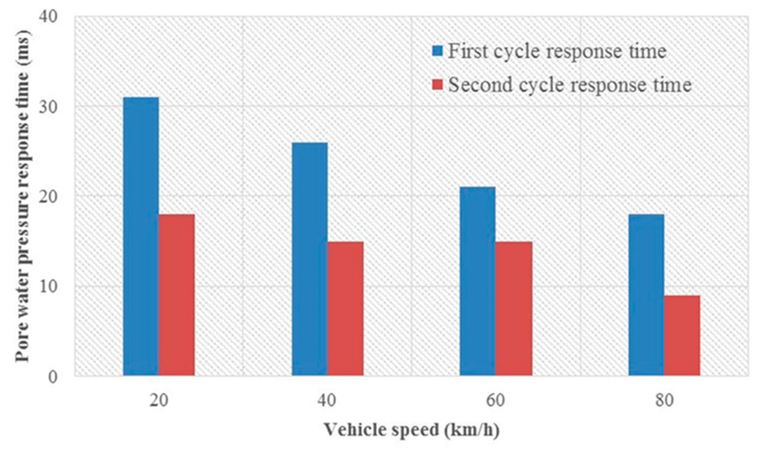
4.2. Analysis of Relationship between Pore water Pressure Response Time and Vehicle Speed

As can be seen from Figure 6, there are two obvious cycles in the pore water pressure response curve at different vehicle speeds. The pore water pressure response time at different speeds are listed in

Table 6. The relationship between pore water pressure response time and vehicle speed.

Vehicle Speed (km/h)	First Cycle Response Time	Second Cycle Response Time	Pore Water Pressure Response Time (ms)	Vehicle Loading Time (ms)
20	31	18	49	36.5
40	26	15	41	15.8
60	21	15	36	10.5
80	18	9	27	7.9

.

Table 6 shows that the pore water pressure response time is longer than vehicle loading time, indicating that even if the vehicle has passed through the pore, the scouring action and pumping action of the free water in the pore on the pore sidewall does not end immediately, but continues for a while. The higher the speed, the greater the ratio of the pore water pressure response time and vehicle loading time. For example, when the speed of the vehicle is 20 km/h, the pore water pressure response time is 1.34 times that of vehicle loading time, and the corresponding data at the speed of 80 km/h is 3.4 times. The time of two cycles at different speed is drawn in the Figure 8.

At a certain speed, the first cycle response time is longer than the second cycle response time, and the first cycle response time is generally 1.5 to 2 times that of the second cycle response time. At different speeds, the first cycle response time and the second cycle response time gradually decreases as the vehicle speed increases. Therefore, as the vehicle speed increases, the scouring time for the pavement structure decreases.

5. Conclusions

This study designed a test method for the true pore water pressure of pavement structures. Then, based on the measured data, the following can be concluded:

(1)

A practical pore water pressure test method for saturated asphalt pavement is designed. The advantage is mainly that the structure of the asphalt pavement is less disturbed and the measured data is closer to the actual value.

(2)

Based on the analysis of hydrodynamic water hammer theory, it is concluded that the pore water pressure shows a periodic decay phenomenon with time, and the decay phenomenon is analyzed. Finally, the empirical formula of maximum positive pressure with speed and the empirical formula of Abp at different speeds are obtained.

(3)

Measurement data show that the pore water pressure gradually increases with increasing vehicle speed, and the pore water pressure response time becomes shorter.

To date, dynamic water erosion damage remains the main form of pavement damage, so the research results of this article can provide data support for subsequent research and provide guidance for pavement structural forms in actual construction. Of course, there are many factors that cause road water damage, which will be the focus of future research.

References

1. Apeagyei, A.K.; Grenfell, J.R.A.; Airey, G.D. Evaluation of moisture sorption and diffusion characteristics of asphalt mastics using manual and automated gravimetric sorption techniques. J. Mater. Civ. Eng. 2014, 26, 839–844. [Google Scholar] [CrossRef]
2. Tarefder, R.A.; Ahmad, M. Evaluating the relationship between permeability and moisture damage of asphalt concrete pavements. J. Mater. Civ. Eng. 2015, 27, 41–72. [Google Scholar] [CrossRef]
3. Jahromi, S.G. Investigation of damage and deterioration hazard in asphalt mixtures due to moisture. Proc. Inst. Civ. Eng. Transp. 2018, 171, 98–105. [Google Scholar] [CrossRef]
4. Min, H.G.; Zhang, W.P.; Gu, X.L. Effects of load damage on moisture transport and relative humidity response in concrete. Constr. Build. Mater. 2018, 169, 59–68. [Google Scholar] [CrossRef]
5. Kim, S.-H.; Kim, N.; Jeong, J.-H. Use of Surface Free Energy Properties to Predict Moisture Damage Potential of Asphalt Concrete Mixture in Cyclic Loading Condition. KSCE J. Civ. Eng. 2003, 7, 381–387. [Google Scholar] [CrossRef]
6. Bozorgzad, A.; Kazemi, S.F.; Nejad, F.M. Evaporation-induced moisture damage of asphalt mixtures: Microscale model and laboratory validation. Constr. Build. Mater. 2018, 171, 697–707. [Google Scholar] [CrossRef]
7. Abuawad, I.M.A.; Al-Qadi, I.L.; Trepanier, J.S. Mitigation of moisture damage in asphalt concrete: Testing techniques and additives/modifiers effectiveness. Constr. Build. Mater. 2015, 84, 437–443. [Google Scholar] [CrossRef]
8. Kringos, N.; Scarpas, A.; Bondt, A.D. Determination of moisture susceptibility of mastic stone bond strength and comparison to thermodynamical properties. Tech. Sess. Assoc. Asph. Paving Technol. 2008, 77, 435–478. [Google Scholar]
9. Weldegiorgis, M.T.; Tarefder, R.A. Towards a Mechanistic Understanding of Moisture Damage in Asphalt Concrete. J. Mater. Civ. Eng. 2015, 27, 0899–1561. [Google Scholar] [CrossRef]
10. Arambula, E.; Caro, S.; Masad, E. Experimental measurement and numerical simulation of water vapor diffusion through asphalt pavement materials. J. Mater. Civ. Eng. 2010, 22, 588–598. [Google Scholar] [CrossRef]
11. Khalili, N.; Selvadurai, A.P.S. On the constitutive modeling of thermo-hydro-mechanical coupling in elastic media with double porosity. In Elsevier Geo-Engineering Book Series; Elsevier: Amsterdam, The Netherlands, 2004; Volume 2, pp. 559–564. [Google Scholar] [CrossRef]
12. Kettil, P.; Engstrom, G.; Wiberg, N.E. Coupled hydro-mechanical wave propagation in road structures. Comput. Struct. 2005, 83, 1719–1729. [Google Scholar] [CrossRef]
13. Cai, Y.Q.; Cao, Z.G.; Sun, H.L. Dynamic response of pavements on poroelastic half-space soil medium to a moving traffic load. Comput. Geotech. 2009, 36, 52–60. [Google Scholar] [CrossRef]
14. Gao, J.; Guo, C.; Liu, Y. Measurement of pore water pressure in asphalt pavement and its effects on permeability. Measurement 2015, 62, 81–87. [Google Scholar] [CrossRef]
15. Cui, X.; Zhang, J.; Huang, D. Analysis of Vehicle-Force-Induced Dynamic Pore Pressure in Saturated Pavement with LSPM Drainage Base. J. Test. Eval. 2017, 45, 294–302. [Google Scholar] [CrossRef]
16. Novak, M.E.; Birgisson, B.; Mcvay, M. Effects of vehicle speed and permeability on pore pressures in hot- mix asphalt pavement. In Proceedings of the 2nd MIT Conference on Computational Fluid and Solid Mechanics, Cambridge, MA, USA, 17–20 June 2003; pp. 532–536. [Google Scholar]
17. Guo, X.D.; Sun, M.Z.; Dai, W.T. Analysis of effective pore pressure in asphalt pavement based on computational fluid dynamics calculation. Adv. Mech. Eng. 2017, 9, 1–14. [Google Scholar] [CrossRef]
18. Luo, Z.G.; Ling, J.M.; Zhou, Z.G.; Zheng, J.L. Calculation of interbedded pore water pressure of asphalt concrete pavement. Highway 2005, 50, 86–89. [Google Scholar]
19. Luo, S.P.; Dan, H.C.; Li, L. Coupled hydro-mechanical analysis of saturated asphalt pavement under moving traffic loads. J. South China Univ. Technol. 2012, 40, 104–111. [Google Scholar]
20. Dong, Z.J.; Tan, Y.Q.; Cao, L.P. Research on pore pressure within asphalt pavement under the coupled moisture-loading action. J. Harbin Inst. Technol. 2007, 39, 1614–1617. [Google Scholar]
21. Wang, S.R.; Liu, T.W.; Peng, T.G. Water Hammer Theory and Water Hammer Calculation; Tsinghua University Press: Beijing, China, 1980; Volume 62, pp. 57–98. [Google Scholar]
Figure 1. Schematic diagram of a tire passing through a road section p.
Applsci 10 01416 g001
Figure 2. Shape of sensor.
Applsci 10 01416 g002
Figure 3. (a) Section of the model, (b) Top view of the model.
Applsci 10 01416 g003
Figure 4. The photo of field measurement.
Applsci 10 01416 g004
Figure 5. The variation of pore water pressure with time at different speeds.
Applsci 10 01416 g005
Figure 6. Pore pressure propagation diagram.
Applsci 10 01416 g006
Figure 7. The relationship between Abp and time at the speed of 20 km/h.
Applsci 10 01416 g007
Figure 8. The time of two cycles at different speed.
Applsci 10 01416 g008