Frequency Domain Full Waveform Inversion Method of Acquiring Rock Wave Velocity in Front of Tunnels

Abstract

Ahead geological prospecting, which can estimate adverse geology ahead of the tunnel face, is necessary in the process of tunnel construction. Due to its long detection range and good recognition effect on the interface, the seismic method is widely used in tunnel ahead prospecting. However, the observation space in tunnels is quite narrow compared to ground seismic prospecting, which leads to some problems in the acquisition of wave velocity, including: the velocity of the direct wave is used to replace the wave velocity of the forward rock approximately; the arrival time information of seismic waves is the main factor in time-travel inversion or the tomography method, which is sufficient to provide a simple model rather than deal with complex geological conditions. In view of the above problems, the frequency domain full waveform inversion method in ground prospecting is introduced to tunnel seismic prospecting. In addition, the optimized difference format is given according to the particularity of the tunnel environment. In this method, the kinematics and dynamics of the seismic wavefield are fully used to obtain more accurate wave velocity results. Simultaneously, forward modeling and inversion simulations on tunnel samples with typical adverse geological bodies are given here, which verified the validity and reliability of the proposed method.

1. Introduction

With the expanding Chinese economy, many tunnels are being designed and constructed. However, when tunneling in hazardous geologic terrain, with faults, fractures, water-bearing openings, and other adverse geological conditions, construction safety is seriously endangered [1]. The ahead geophysical prospecting method is the main good method to ensure the safety of tunnel construction. The commonly used methods include the seismic ahead prospecting method [2,3], electromagnetic ahead prospecting method, etc. The main electromagnetic ahead prospecting methods include GPR (Ground-penetrating radar) [4,5], transient electromagnetic method [6,7], NMR (nuclear magnetic resonance) [8], etc.

Among the above methods, the seismic ahead prospecting method has the advantages of long prospecting distance, good structure recognition effect, and sensitivity to the interface of undesirable geological bodies [9]. Therefore, it is often used for medium- and long-distance prospecting in tunnel ahead prospecting. Since the 1990s, various seismic methods have been popularized and applied in engineering. Initially, the tunnel seismic wave method was mainly used and referred to surface seismic methods such as Vertical Seismic Profiling (VSP) and the multi-wave train exploration method. Based on VSP, some scholars have proposed and developed Horizon Sound Profiling (HSP) [10]. In this method, the reflected wave signal is analyzed in the time domain and frequency domain, and the geological conditions in front of the tunnel are inferred by combining with geological survey. The Seismic Ahead Prospecting (SAP) system, which has the advantages of flexible layout and convenient operation, is suitable for deployment in the narrow space of a tunnel. At present, the most commonly used seismic wave detection method in tunnel construction is the Tunnel Seismic Prediction (TSP) method developed by Swiss Amberg Measurement Technology Co. Ltd (Switzerland, Regensdorf-Watt). By disposing the collected seismic data with the methods of band-pass filtering, first arrival picking, energy balance, reflection wave extraction, wavefield separation, velocity analysis, and depth migration, the distribution of the front adverse geological body and the mechanical parameters of the rock can be obtained. Although the above methods can detect the undesirable geological body in front of the tunnel more accurately, the wave velocity distribution of the geological body cannot be obtained.

The Full Wave Inversion (FWI) method, which has the characteristics of high precision and high resolution, makes full use of the dynamic and kinematic information of seismic waves. It can accurately characterize the complex underground structures and invert the physical parameters of the earth’s medium. In the 1980s, Lailly and Tarantola proposed generalized least squares FWI in the time domain [11,12,13,14,15,16,17], drawing on Claerbout’s idea of reverse-time offset [18]. In this paper, the gradient of the objective function is obtained via cross-correlation of the forward wavefield and the back-propagated wavefield with the data residual as the seismic source, which avoids the direct calculation of the Frechet derivative. In the 1990s, Pratt et al. [19,20,21,22,23] developed FWI from the time domain to the frequency domain and realized multi-scale inversion from low frequency to high frequency, which lays the foundation for FWI in the frequency domain. Hu [24] combined time domain forward simulation and frequency domain inversion reconstruction algorithms. Modrak and Tromp [25] applied the Limited memory Broyden Fletcher Goldfarb Shanno (LBFGS) algorithm to FWI and proved that its convergence speed is fast and easy to achieve. Luan and Tamara [26] studied a method of using elastic FWI to locate and characterize the disturbance zone in front of the tunnel. However, there is a lack of frequency domain research.

The traditional velocity analysis in tunnels and travel-time tomography methods can only obtain the macroscopic velocity distribution and it is difficult to obtain high-resolution velocity models. FWI method is introduced into the tunnel seismic ahead prospecting method in this study. The frequency domain FWI method was used to study the wave velocity acquisition method of the rock mass in front of the tunnel face. The difference scheme is optimized to make it suitable for the complex environment of the tunnel. The forward data is used to verify the velocity results obtained by the FWI, and a more reliable wave velocity distribution is obtained.

2. Method

According to the realizing domain, FWI can be divided into time domain, frequency domain, and Laplace domain. Time domain FWI is relatively easy to implement, but it cannot effectively achieve multi-scale inversion from long wavelength to short wavelength, and the inversion tends to fall into local small values [27]. The laplace domain FWI method [28] reduces the possibility of inversion problems falling into local minima. In contrast, the frequency domain FWI has a natural multi-scale. With low-frequency inversion to obtain the initial model and mid- to high-frequency inversion of medium wave-number and short wavelength information, it can obtain more accurate physical properties of the underground medium. Therefore, this article mainly introduces the frequency domain FWI method into the field of tunnel ahead prospecting. Combined with the special environment of the tunnel, more accurate wave velocity information of the rock in front of the tunnel face is obtained.

2.1. Frequency Domain Finite Difference Scheme and Boundary Conditions

In wave equation forward modeling, at least three forward simulations are required in each iteration to obtain the gradient operator. Therefore, the correctness of the forward numerical simulation plays an important role in the final inversion result. In the two-dimensional Cartesian coordinate system, the frequency domain acoustic wave equation of a homogeneous isotropic medium is shown as follows [29]:

$${\nabla }^{2}P\left(x,z,w\right)+\frac{w^2}{v^2}p\left(x,z,w\right)=-S\left(w\right),$$

(1)

where ${\nabla }^{2}P\left(x,z,w\right)$ is the Laplace operator, $p$ is the wavefield value of each point in the medium, $w$ is the angular frequency, $v$ is the medium velocity, $S\left(w\right)$ is the source term.

Due to the small range and scale of detection in tunnel space, the optimized nine-point difference scheme proposed by Jo et al. [30] can meet the requirements of difference accuracy. The difference form of the acoustic wave equation is shown in Equation (2) and the diagram of the difference scheme is shown in Figure 1.

$$\begin{array}{c}\Delta \mathrm{x}=\Delta \mathrm{z}=\Delta \\ a\times \left(\frac{P_{m+1,n}+P_{m,n-1}-4P_{m,n}+P_{m,n+1}+P_{m-1,n}}{{\Delta }^2}\right)+\left(1-a\right)\left(\frac{P_{m+1,n+1}+P_{m-1,n+1}-4P_{m,n}+P_{m+1,n-1}+P_{m-1,n-1}}{{\left(\sqrt{2}\Delta \right)}^2}\right)+\\ \frac{w^2}{v^2}\left(\begin{array}{c}c{P}_{m,n}+d\left(P_{m+1,n}+P_{m,n-1}+P_{m,n+1}+P_{m,n-1}\right)+\\ e\left(P_{m+1,n+1}+P_{m-1,n+1}+P_{m+1,n-1}+P_{m-1,n-1}\right)\end{array}\right)=-S\left(w\right)\end{array}$$

(2)

Compared with ground seismic exploration, the scale of research in the tunnel environment is relatively small; at the same time, the wavelength of low frequency information is longer. Thus, it is necessary to increase the boundary thickness to reduce the boundary reflection, which greatly increases the calculation amount. For the above problems, the Complex Frequency-Shifted Perfectly Matched Layer (CFS-PML) is used to enhance the absorption of boundary reflection [31,32]. Its basic form is as follows:

$$S_x\left(x\right)={\beta }_x\left(x\right)+\frac{d_x}{{\partial }_x\left(x\right)+iw},$$

(3)

$${\partial }_x\left(x\right)={\partial }_0\left(1-\left(\frac{x}{L}\right)\right),$$

(4)

$${\beta }_x\left(x\right)=1+\left({\beta }_0-1\right){(\frac{x}{L})}^2,$$

(5)

$$d_x\left(x\right)=d_0{(\frac{x}{L})}^2,$$

(6)

where d directly acts on the matching layer and enables the medium to decay in the form of exponential so that PML can obtain a better absorption effect. $\partial$’s function is to suppress the converted wave generated at the boundary of the medium perfectly matched layer by the generated light wave. β indirectly increases the absorption capacity of PML by increasing the incident angle of the light wave.

2.2. Frequency Domain FWI

Inversion is the process of obtaining geophysical parameters by inverting the wavefield based on the actually observed seismic data. Actually, inversion is a process of local optimization. By continuously updating the initial model, the real model can be approximated to the maximum to obtain the global optimal solution.

2.2.1. Build Objective Function

The objective function is obtained by minimizing the difference between the forward data and the observation data, thereby obtaining the best model data. Brossier [33] compared four minimization functions. Experimental tests show that the L2 norm is a relatively stable objective function when dealing with noisy data with the best inversion effect. Therefore, this paper adopts the objective function based on the L2 norm for inversion.

When the wavefield residuals of field observation seismic records and forward seismic records obey Gaussian distribution, the objective function based on the L2 norm is [33]:

$$E\left(v\right)=\frac{1}{2}{\Vert d_{obs}-d_{mod}\Vert }^2=\frac{1}{2}\Delta d^T\Delta d^{*},$$

(7)

where d_obs is the field observation seismic data, d_mod is the full wavefield seismic record obtained from forward modeling, d_mod is the function of the speed model v, $\Delta d$ is the wavefield residual between the observation data and the calculated data, T is the transpose operator, and * represents conjugate.

2.2.2. Gradient Operator and Step Size

The adjoint state method is the common gradient operator computing method in FWI, which can avoid extra calculation consumption. We apply the second-order Taylor-Lagrange expansion to the objective junction E(v) at v₀. Then, we take the first-order derivative with respect to v at both sides of the approximation. The adjoint state is defined by $\frac{\partial E\left(v\right)}{\partial v}=0.$ [34]:

$$\left[\mathrm{Re}(H\right)+\lambda {\rm I}]\delta v=-\mathrm{Re}(G^T\Delta d^{*}),$$

(8)

where $H\approx G^T{G}^{*}$ is an approximate Hessian matrix, G is a Jacobian matrix, I is a unit matrix, and $\lambda$ is a regularization parameter. There is one adjoint system per shot and per angular frequency. The matrix A propagates the shot into the earth and u_s is the incident field originating at s. ${\lambda }_s$ is the backpropagation of the residual field. The gradient operator in the frequency domain is [35]:

$$\nabla E=-\mathrm{Re}({{\displaystyle \sum }}_{\omega }{{\displaystyle \sum }}_s{\lambda }_s,\frac{\partial A}{\partial v}{u}_s{}_x).$$

(9)

The iterative step length is obtained using the method of line search. There are two main line search methods: imprecise search method and parabolic search method. This article adopts the two-point parabolic search method, and the process is as follows.

First, a forward wavefield simulation is required. We give a global trial step size ${\alpha }_0$ (usually 1% of the background speed). A pseudo-update velocity field $v_p=v_0-{\partial }_{0}g$ is obtained at the update rate, and a finite difference forward numerical simulation is performed on the pseudo-update velocity field. Calculate the forward and back propagation wavefield and obtain the pseudo-velocity field objective function $E\left(v_p\right)$, and do a second-order Taylor expansion around it:

$$E\left(v_p\right)=E\left(v\right)-{\alpha }_0\left(g\left(v\right),g\left(v\right)\right)+\frac{{\alpha }^2{}_0}{2}\tau =E\left(v\right)-{\alpha }_{0}g{\left(v\right)}^2+\frac{{\alpha }^2{}_0}{2}\tau ,$$

(10)

where $\tau$ is a value related to the second derivative of the error norm with respect to velocity. In the case of the current error function $E\left(v\right)$, the error function based on the pseudo-velocity field $E\left(v_p\right)$, and the test step known, the $\tau$ can be calculated:

$$\tau =2\frac{E\left(v_p\right)-E\left(v\right)+{\alpha }_{0}g{\left(v\right)}^2}{{\alpha }_0{}^2}.$$

(11)

If there is an optimal step size $\alpha$, it must meet $\nabla E\left(\alpha \right)=0$. The second-order Taylor expansion of the error function of the optimal step is expanded in the same form as speed, at which point the optimal step size is:

$$\alpha =\frac{g{\left(v\right)}^2}{\tau }.$$

(12)

2.2.3. LBFGS Algorithm

This paper adopts an improved quasi-newton algorithm LBFGS to optimize the algorithm, which occupies less computing memory and does not need to store Hessian matrices. It has second-order convergence and low computational complexity. The algorithm is constructed in the following steps:

• First, give a simple positive definite matrix $H_k^{\left(0\right)}$, generally using Equation (13) given by Nocedal [36]:

  $$H_k^{\left(0\right)}=\frac{s_k^T{y}_k}{|\left|y_k\right|{|}^2}I.$$

  (13)
• The construction form of the pseudo-Hessian operator with limited memory in the LBFGS algorithm is shown below:

  $$H_k^{\left(j+1\right)}=\left(I-\frac{sk{y}_k^T}{s_k^{T}yk}\right)H_k^j\left(I-\frac{yk{s}_k^T}{s_k^{T}yk}\right)+\frac{sk{s}_k^T}{s_k^{T}yk},j=0,1,\dots ,m,$$

  (14)

  where $s_k$ is the update amount of the speed model v, $y_k$ is the update amount of the gradient, $H_k^j$ is the Hessian operator with limited memory obtained for the kth time, and m is the dimension of the speed update amount and the gradient update amount. The larger the m, the larger the amount of calculation and memory storage, and the higher the inversion accuracy. Generally, the value range of m is [5, 30].
• Let ${\rho }_k=\frac{1}{s_k^T{y}_k}$, $V_k=\left(I-{\rho }_k{y}_k{s}_k^T\right)$; substituting into Equation (14) can get the pseudo-Hessian operator expression. After recurrence, we can know the relationship between the pseudo-Hessian operator of the (k + 1)th iteration and the positive definite Equation (12) given at the beginning.

  $$\begin{array}{c}{H}_{k+1}=H_k^{\left(m+1\right)}=\left(m_k^T\dots m_{k-m}^T\right)H_k^{\left(0\right)}\left(m_{k-m}\dots m_k\right)+\\ {{\displaystyle \sum }}_{j=0}^m\rho k-m+j\left({{\displaystyle \prod }}_{l=0}^{m-j-1}{m}_{k-l}^T\right)sk-m+j{s}_{k-m+j}^T\left({{\displaystyle \prod }}_{l=0}^{m-j-1}{m}_{k-l}^T\right).\end{array}$$

  (15)

According to Equation (15), it can be seen that the LBFGS algorithm only needs to store $m+1$ times of speed update amount, $sk$, and gradient update amount, $yk$. In this way the pseudo-Hessian matrix $H_{k+1}$ required for the construction of the descent direction can be calculated. It only uses the information of the first-order partial derivative in the process of constructing the Hessian matrix and reduces the complexity of the calculation. The inversion accuracy of the LBFGS method is higher than the gradient method.

2.3. Frequency Selection Strategy

It is very important to select the appropriate frequency components for frequency domain FWI. Too few frequency components will lead to instability of the inversion and it will be easy to fall into local minima. However, too many frequency components can not only increase the accuracy of inversion but also increase redundant computation and waste memory space and calculation time.

Sirgue [37] and Pratt [38] discussed several factors that affect frequency selection in waveform inversion such as wave-number, offset, and the frequency selection strategy. In order to maintain the continuity of wave-number, the frequency selection formula should be as shown below:

$$f_{k+1}=\frac{f_k}{{\alpha }_{\min }},$$

(16)

$$\Delta f_{k+1}=f_{k+1}-f_k=\frac{1-{\alpha }_{\min }}{{\alpha }_{\min }}{f}_k.$$

(17)

Equations (16) and (17) show that the optimal frequency increment is not a constant but increases with the frequency increases. This section assumes that the optimal frequency selection method is obtained under the condition that the medium is in a geological model with uniform velocity in one dimension. In ahead geological prospecting in a tunnel, the selected frequency is increased appropriately according to the tunnel observation mode and the detection distance, which is beneficial to improve the detection resolution due to the limited observation method.

The flow chart of the adjusted frequency domain FWI method, which can realize accurate detection of adverse geological bodies in front of the tunnel, is shown as Figure 2.

3. Numerical Simulation

Due to the complexity of the underground geological conditions, various undesirable geological bodies will be encountered during tunnel construction, which will do harm to the construction. The undesirable geological structures often encountered in tunnel construction mainly include lithological interfaces, fault fracture zones, karst geological bodies, composite strata, etc. [39]. They are further explained in

Table 1. The explanations of undesirable geological structures in tunnels.

Geological Structures	Further Explanations
Lithologic interface	The rock interface of two different lithology.
Fault fracture zone	In the process of fault formation, fracture of surrounding rock is often caused by the dislocation of upper and lower plates, forming a fault fracture zone.
Karst geological body	Karst systems such as caverns and crevices often exist in karst areas. Cavities created by the long-term dissolution of groundwater are called caverns.
Composite strata	For instance, Wedge bad geological bodies, a group of caverns consisting of multiple caverns, etc.

.

The tunnel cavity will interfere with ahead prospecting of seismic waves. Therefore, forward simulation of seismic ahead prospecting should be carried out firstly without anomalous objects in front of the tunnel face, and the influence of the tunnel cavity on the forward simulation results should be studied. This is also conducive to the identification of the seismic wavefield response characteristics of typical undesirable geological bodies in the next part. The observation system is shown in Figure 3.

3.1. Geological Interface Model

The lithologic interface models with a 90° and 45° dip angle are established respectively (Figure 4a,b). The size of the forward model is 160 m × 80 m and grid spacing is $\Delta x=\Delta y=1m$. The CFS-PML absorption boundary around the model is set. Referring to the tunnel size in the actual project, the tunnel size in the forward model is set to length 50 m × width 12 m and the tunnel cavity is filled with air. The rock wave velocity on one side of the tunnel is set to 4000 m/s and the rock wave velocity in front of the lithological interface is set to 2000 m/s. The seismic source adopts Ricker wavelet, and the main frequency is 200 Hz. The sampling interval of the detector is 0.005 ms.

Figure 5a,b shows the Common Source Point (CSP) gather seismic records of the common shot gather of all the lower side wall geophones selected as the seismic source at a distance of 5 m from the tunnel face of the lower side wall. In order to make the reflected waves in the seismic records clearer, the interference of the tunnel cavity and the tunnel surface scattered wave are removed. In other words, here the original seismic records of no anomalous bodies in front of the tunnel are subtracted from the 90° and 45° dip angle lithology interface model CSP gather seismic records. In Figure 5a, it can be seen that the seismic wave detection response characteristic of 90° lithologic interface is a continuous homogeneous axis of inclined straight line. The weaker homogeneous axes at the back is caused by multiple reflections of the reflected wave between the 90° lithologic interface and the tunnel face.

The frequency domain FWI is carried out via the observation mode shown in Figure 3 and the results are shown in Figure 6a,b. The actual engineering pays more attention to the geological conditions of the unexcavated section; consequently, only the wave velocity in front of the tunnel face is updated here. There is an obvious wave velocity interface in the figure, and its position corresponds well to the position of the real lithological interface (white dotted line). It can be seen that the inversion result can basically reflect the position and shape of the lithological interface. In terms of the accuracy of the inverted wave velocity value, there is a wave velocity transition zone near the interface, and the inverted wave velocity at other locations is slightly higher than the actual situation. On the whole, the inversion wave speed is close to the real wave speed, and it reflects the changing trend of wave speed from high to low, which has a good guiding role for construction.

3.2. Fault Model

A fault model with a thickness of 30 m is established (Figure 7a). The size of the forward model is 160 m × 80 m, and grid spacing is $\Delta x=\Delta y=1m$. The CFS-PML absorption boundary around the model is set. Referring to the tunnel size in the actual project, the tunnel size in the forward model is set to length 50 m × width 12 m and the tunnel cavity is filled with air. The inclination angle of the fault is 75° and the distance from the tunnel face is 30 m. The rock wave velocity on one side of the tunnel is set to 4000 m/s and the rock wave velocity inside the fault is set to 2000 m/s. Another fault model with a thickness of 110 m is established (Figure 7b). The size of the forward model is 175 m × 80 m, and the inclination angle of the fault is 60°.

Figure 8 shows the CSP seismic records of the common shot gather of all the lower wall geophones with the lower wall 5 m away from the tunnel face selected as the seismic source in the 30 m thick fault model. The original seismic records of no anomalous body in front of the tunnel face are also subtracted in order to remove the interference of scattered waves from the tunnel cavity and the tunnel face. From Figure 8, it can be seen that the response characteristic of the fault is a strong event axis and a set of weaker event axes. The strongest event axis corresponds to the front interface of the fault. There are multiple weaker event axes. After analysis, it is believed that it is caused by the mixing of the reflected wave at the back interface of the fault and the secondary reflected wave at the front interface.

The frequency domain FWI is carried out via the observation mode shown in Figure 3. The results are shown in Figure 9a,b. In addition, only the wave velocity of the front of the tunnel face is updated. The white dashed line in the figure represents the position and shape of the real lithologic interface. The front and back interfaces of the fault are retrieved and the position and inclination of the interface are more accurate. The wave velocity inside the fault is close to the real wave velocity except for the low wave velocity in some regions.

3.3. Karst Geological Model

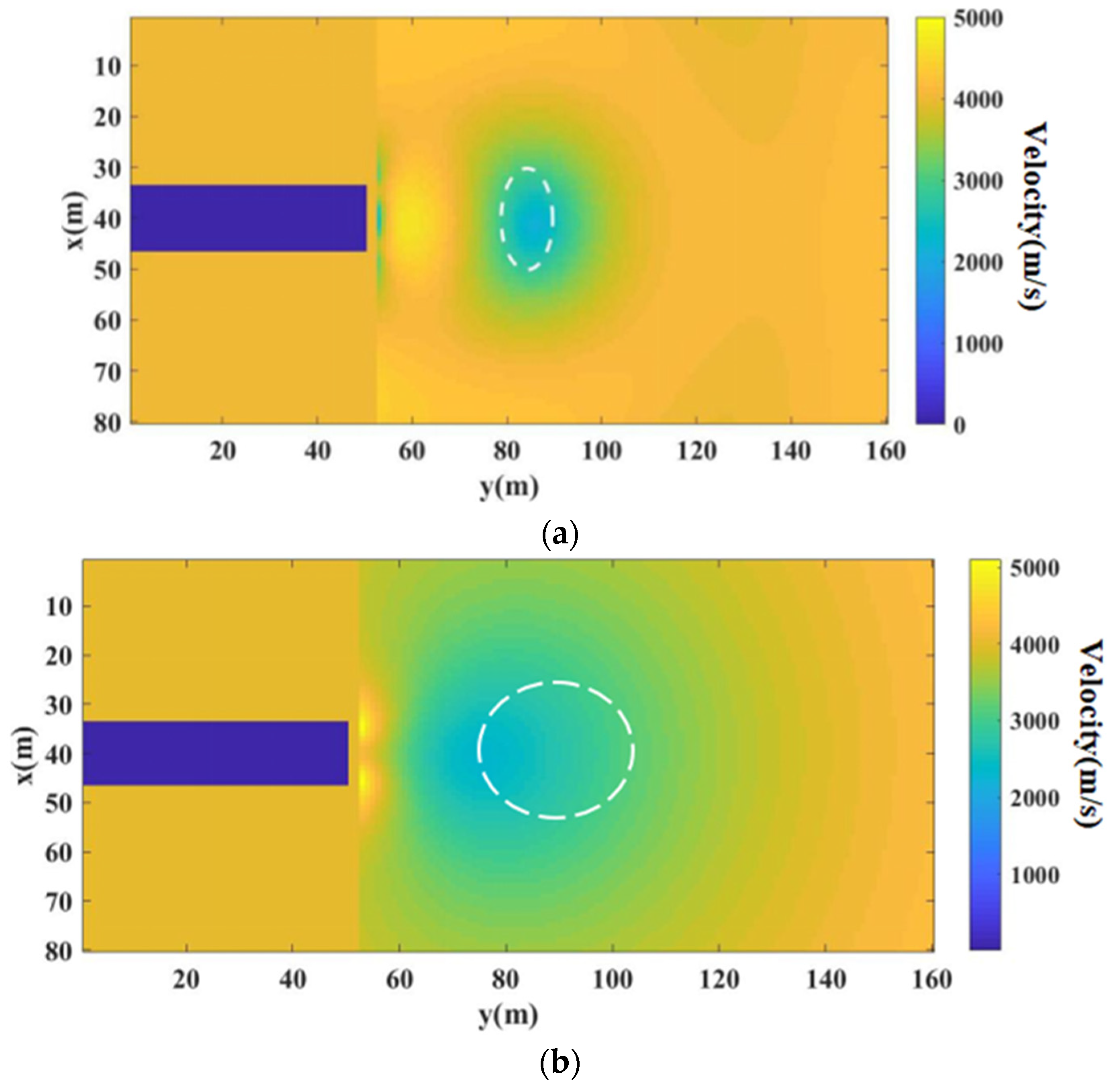
The karst geological models with a thickness of 10 m and 30 m are established respectively (Figure 10a,b). The size of the forward model is 160 m × 80 m, and the grid spacing is $\Delta x=\Delta y=1m$. The CFS-PML absorption boundary around the model is set referring to the tunnel size in the actual project. The tunnel size in the forward model is set to length 50 m × width 12 m and the tunnel cavity is filled with air. The cavern is elliptical with a width of 20 m up and down, a thickness of 10 m left and right, and the nearest point of the front interface is 30 m away from the tunnel face. The wave velocity of the surrounding rock of the tunnel is set to 4000 m/s. The cave is filled with broken rock mass, and the wave velocity is 2000 m/s.

Figure 11a,b show the CSP seismic records of the common shot gathers of all the lower wall geophones with the lower wall 5 m away from the tunnel face selected as the seismic source in the karst cave model with a diameter of 10 m and 30 m. The original seismic records of no anomalous body in front of the tunnel face are also subtracted. It can be seen that the three sets of strong event axes all show the characteristics of weaker energy as the distance between the geophone and the cavern increases. The first strong event axis corresponds to the front interface of the cave. The second group of events consists of two phase axes, corresponding to the back interface of the cave. The third phase axis and the following multiple weak phase axes are considered to be multiple reflection waves and diffracted waves after analysis.

The frequency domain FWI is carried out via the observation mode shown in Figure 3, and the results are shown in Figure 12a,b. In addition, only the wave velocity of the front of tunnel face is updated. A white dotted line represents the position and shape of the real lithologic interface. It can be seen that the inversion results of the cave with a diameter of 20 m are ideal, the position and shape of the cave inversion are more accurate, and the wave velocity inside the cave is very close to the real wave velocity. In the inversion result, there is a wave velocity interface between the cave and the surrounding rock, which makes the cave slightly larger. Overall, the location of the cavern is accurate and easy to identify, which can provide good guidance for construction.

4. Discussion

This paper mainly discusses the forward and inverse problems in the frequency domain FWI. First, the nine-point difference scheme is used in frequency domain wave equation forward modeling. Compared to the large-grid forward simulation on the ground, the nine-point difference scheme not only meets the accuracy requirements, but also greatly reduces the calculation amount and improves calculation efficiency. The tunnel ahead prospecting has a smaller scale than the seismic exploration on the surface, so the boundary condition needs to be more detailed. The CFS-PML boundary condition is adopted to effectively suppress the boundary false reflection and ensures the accuracy of the forward modeling. In the inversion process, the objective function is initially established. The FWI gradient formula is obtained using the adjoint state method, which greatly reduced the calculation amount compared with the Jacobian matrix derivation. The parabola method is used to obtain the optimized step length, thereby speeding up the convergence speed. In the optimization algorithm, the LBFGS algorithm is used to perform local optimization solutions, which greatly reduces the amount of calculation and storage while ensuring high accuracy. Finally, the theoretical framework of FWI is established.

In the research of several typical undesirable geological numerical examples, we have explored some rules. For the lithological interface, if the dip angle is large (90°), the FWI method can give the accurate position and shape of the lithological interface. The inversion value of the rock and wave velocity behind the interface is also accurate. For a small inclination interface (45°), the FWI method cannot give the accurate position and shape of the interface. The rock wave velocity inversion behind the interface also has a certain error. However, it can still give an accurate wave velocity change trend, which can provide guidance for construction. For faults, the position of the interface before and after the fault and the approximate wave velocity of the internal rock mass can be accurately given. When the thickness of the fault is small, the upper part of the fault has a certain distortion and the inversion result will be further deteriorated when the thickness of the fault is further reduced. For karst caves, the location, shape, and approximate wave speed of the internal rock mass can be inverted accurately. However, when the cave is small, the FWI method can only invert the presence of low-velocity anomalies in front of the cave, and the specific position and shape cannot be obtained. As the size of the cave is further reduced, the effect will be further deteriorated.

This paper only studies the two-dimensional FWI method in tunnels. Actually, ahead prospecting of tunnel engineering is a three-dimensional full-space problem. Thus, the three-dimensional FWI method in tunnels needs to be studied further. However, the FWI method has a large amount of calculation and long calculation time, which does not meet the requirement of rapid construction in the project. Therefore, more effective parallel methods should be studied continuously to improve the computing efficiency and increase the practicality of the three-dimensional FWI method in tunnels in future work.

5. Conclusions

Aiming at the problem of insufficient wave velocity calculation accuracy of the commonly used inversion method for complex geological models, this paper introduces the frequency domain FWI method into seismic ahead prospecting in tunnels and carries out the corresponding method. The adjustment and optimization make it suitable for the complex environment in a tunnel and can calculate more accurate wave velocity results, which lays the foundation for the subsequent acquisition of imaging results and compressive strength distribution results.

Due to the complexity of the underground geological conditions, various undesirable geological conditions will be encountered during tunnel construction, which will do harm to the construction. This paper chooses several types of typical undesirable geological bodies commonly encountered in tunnel construction and establishes models of lithological interfaces, faults, and karst caves. In terms of the imaging effect of the frequency domain FWI, the analysis of its advantages and shortcomings is given. The forward simulation and FWI study of tunnel seismic wave ahead prospecting were carried out, which verified the validity and reliability of the method in this paper. It provided a basis for the detection and geological interpretation of typical undesirable geological bodies in actual engineering.