Spectral-Element Simulation of the Turbulent Flow in an Urban Environment

Abstract

The mean flow and turbulence statistics of the flow through a simplified urban environment, which is an active research area in order to improve the knowledge of turbulent flow in cities, is investigated. This is useful for civil engineering, pedestrian comfort and for health concerns caused by pollutant spreading. In this work, we provide analysis of the turbulence statistics obtained from well-resolved large-eddy simulations (LES). A detailed analysis of this database reveals the impact of the geometry of the urban array on the flow characteristics and provides for a good description of the turbulent features of the flow within a simplified urban environment. The most prominent features of this complex flow include coherent vortical structures such as the so-called arch vortex, the horseshoe vortex and the roof vortex. These structures of flow have been identified by an analysis of the turbulence statistics. The influence of the geometry of urban environment (and particularly the street width and the building height) on the overall flow behavior has also been studied. Finally, the well-resolved LES results were compared with an available experimental database to discuss differences and similarities between the respective urban configurations.

1. Introduction to Urban Flows

The study of complex turbulent flow in an urban environment is of particular interest in various domains and has been an active research area over the past years. Indeed, the presence of buildings affects the flow field and results in complex patterns for the dispersion of scalar quantities, such as contaminants. Thus, the spread of pollution in urban areas is of concern for public health. However, developing predictive models is challenging due to the wide range of factors which can affect the flow field, such as moving cars, population density, trees, buildings or street canyons. Describing the structure of flow through an idealized urban area and the operation of parameterizing it are therefore necessary to have a better understanding of pollutant spreading and to determine predictive models of the evolution in air quality within the city [1]. Although using an idealized urban environment simplifies the real urban flow, it is necessary to focus on the physical mechanisms governing the flow structure and the turbulence characteristics.

The structure of flow through an urban environment has been described by Britter and Hanna [2] both at a local scale and at a larger scale. The wind turbulence in street canyons can affect pedestrian mobility and comfort as studied by Stathopoulos [3], whereas the same wind flow at a larger scale represents the wind environment of the city and is a major factor for the design and implementation of new buildings. It thus affects the removal of exhaust gas and pollution from the urban canopy and is therefore of great interest in order to improve the quality of air within the urban area. Garbero et al. [4] performed wind-tunnel tests to investigate pollutant dispersion as a passive scalar within a street network. The mass transfer between the streets was measured as well as the mean velocity profile of the flow above the urban canopy upon various geometrical conditions in order to emphasize the dependence of these processes on the geometrical properties of the street network. Pollutant dispersion is controlled by turbulent mixing and the mean-flow transport within the street network. The turbulence and the mixing characteristics within such an environment have been investigated by Belcher [5] using direct numerical simulation (DNS). It has been shown that the wind blowing within the urban canopy is slower than the flow above the buildings because of the canopy drag. However, the wind blowing within the streets creates a mixing circulation which favored exchanges of scalar quantities within the urban environment.

Numerous numerical studies have been conducted in order to describe the flow and scalar dispersion within the urban area. Baik and Kim [6] investigated the flow characteristics within urban streets canyons using a two-dimensional numerical model build with the turbulent closure scheme. They described the flow field by the number and intensity of vortices within the street canyons. On the other hand, DNS was performed by Vinuesa et al. [7] for the flow around a wall-mounted square cylinder under various inflow conditions. They highlighted the turbulence features for a laminar-inflow case and for a turbulent-inflow simulation are different; they also studied the horseshoe vortex forming around the square cylinder as it had been observed by Nagib and Corke [8] using smoke-wire visualizations. These phenomena have also been studied experimentally by Monnier et al. [9] in a simplified urban area. Indeed, it is possible to assess the flow characteristics by performing wind-tunnel tests because these experiments enable a good control of the input parameters. They highlighted the multi-scale characteristics of the flow field through a simplified urban environment and identified different features of the flow within this urban array such as the wake, the shear layers and the horseshoe vortex mentioned above. They mainly focused on the structural components of the flow and the impact of factors such as the angle of incidence of the wind in order to describe the flow through an urban array. The turbulence dissipation within the street canyons and the deceleration of the mean flow were emphasized, as well as the features of the flow near the wall.

In this study we perform high-fidelity numerical simulations of the flow through a simplified urban environment and compared them with the experimental results from Monnier et al. [9]. Well-resolved large-eddy simulations (LES) have been performed using the spectral-element code Nek5000 developed by Fischer et al. [10] and post-processed with the statistics toolbox developed by Vinuesa et al. [11]. The result is a complete description of the flow through an array of $3\times 4$ blocks. Next, we will discuss the characteristics of urban flows.

1.1. Structure of the Flow above the Urban Canopy

Urban obstacles such as buildings create a relatively large drag force on the atmospheric boundary layer (ABL). Britter and Hannah [2], as well as Kastner-Klein and Rotach [12], described the structure of the ABL above urban areas with three major sublayers: the urban canopy sublayer, the roughness sublayer and the inertial sublayer. In the so-called inertial sublayer, the turbulent fluxes are almost constant because the boundary layer has adapted to the effect of the urban obstacles. Therefore, it is treated by standard atmospheric boundary layer formulas and, thus, the mean velocity profile can be approximated fairly well by the following logarithmic law:

$${\displaystyle U\left(z\right)=\frac{u_{*}}{\kappa }ln\left(\frac{z-d_0}{z_0}\right),}$$

(1)

where $d_0$ is the displacement height, $z_0$ is the roughness length, $u_{*}$ is the friction velocity and $\kappa =0.4$ is the Von Kármán constant. Note that U is the mean velocity in the streamwise direction and z is the wall-normal coordinate; similarly, V and W are the mean velocity components in the spanwise and the vertical directions, respectively.

Reynolds and Castro [13] used particle-image-velocimetry (PIV) measurements to investigate the flow through an urban environment. They observed that in the outer region the roughness does not significantly affect the mean velocity profiles and the Reynolds-stress profiles. The logarithmic law can adequately model the mean velocity profile in the inertial sublayer. The inflection point identified by Finnigan [14] and later by Belcher et al. [15] using LES in the context of forest canopies was also observed by Reynolds and Castro [13] in the case of urban canopies. This inflection point is at the top of the roughness layer and marks the transition between the roughness layer (where the mean profiles are still disturbed by the roughness elements) and the inertial sublayer (where the mean profiles follow the logarithmic law).

On the other hand, within the urban canopy layer, the flow is directly affected by the urban obstacles and, in the roughness sublayer, the flow is still adjusting to the effects of many obstacles (Kastner-Klein and Rotach [12], Britter and Hannah [2] and Stull [16]). Therefore, within both sublayers, the flow has a rather complex structure. In the vertical direction, the roughness sublayer extends from the ground to a level at which the flow can be taken horizontally homogeneous, as it has been investigated by Finnigan [14], Belcher et al. [15] and Dupont and Brunet [17] using LES in the case of the flow above a forest canopy and by Britter and Hannah [2] and Reynolds and Castro [13] in the urban context. This can occur from 2 times to 5 times the average height of the urban obstacles. Therefore, in areas with high buildings such as most of large American cities, the roughness sublayer represents a significant part of the urban boundary layer. As most of pollution problems occur in this sublayer, predictive models for the spread of pollution require information of the flow structure within the roughness sublayer [4].

1.2. Influence of an Urban Obstacle

The buildings for the urban environment investigated here are represented by wall-mounted cylinders with a square cross-section. A wide range of computational-fluid-dynamics (CFD) and experimental studies have been conducted around such an obstacle in order to describe the flow topology. The flow around a cubical obstacle under a laminar inflow condition was simulated by Liakos and Malamataris [18]. Vinuesa et al. [7] investigated the influence of the inflow conditions by performing DNS and several experimental results report on this, such as the one from Nagib and Corke [8].

The vortical structures of the flow have been investigated experimentally in the following works: Sousa [19], by using digital particle image velocimetry (DPIV) and Hussein and Martinuzzi [20] by using laser Doppler anenometry (LDA). Becker et al. [21] studied the influence of the angle of incidence of the wind on the structure of the flow around a wall-mounted square cylinder. Similarly, Monnier et al. [22] studied the influence of a small angle of incidence and later the influence of a larger angle of incidence [9] on the flow through a simplified urban environment. The urban environment creates a relatively large drag force: The flow is significantly slowed down by the obstacle. Hwang and Yang [23] performed numerical studies with low-to-moderate Reynolds number to describe the vortical structures of the flow around a wall-mounted square cylinder. They highlighted a stagnation point in the flow.

The region very close to the cylinder is significantly disturbed, with large areas of reversed flow: A low velocity region upstream the obstacle and an acceleration region at both side of the obstacle. Within the low-velocity region upstream the obstacle, the flow stagnates and raises to get over the obstacle. This was also discussed in the context of climate models by Schenk and Vinuesa [24]. A wide horseshoe vortex is formed around the cylinder due to the rollup of the incoming boundary layers spanwise vorticity and its interaction with the obstacle. This has been described by several studies and observed experimentally by Nagib and Corke [8] and numerically by Vinuesa et al. [7]. Reynolds and Castro [13] identified a separation saddle point upstream the obstacle. This point marks the upstream limit of this horseshoe vortex, which then curls around the cube. Inside the region downstream of the obstacle, the streamwise velocity slows down because of the drag force created by the obstacle. The adverse pressure gradient formed at the obstacle because the regions of different velocities are responsible for a recirculation bubble downstream of the obstacle near the wall.

High turbulent kinetic energy (TKE) regions are also noticeable on both sides of the obstacle (Vinuesa et al. [7] and Becker et al. [21]) because of the interactions at the wake layer with the shear layer on both sides of the urban obstacle. This increased TKE, mostly due to the streamwise velocity fluctuations, is responsible for the emergence of coherent vortical structures. Many experimental studies investigate the flow around a wall-mounted obstacle characterized by a small aspect ratio: Becker et al. [21], Sousa [19] or Hussein and Martinuzzi [20] used laser Doppler anenometry (LDA) to focus on the energy balance within the turbulent flow.

Many studies proposed a description of the flow topology around the obstacle based on experimental measurements or computational data. They highlighted the two large vortices that are formed on both sides of the obstacle and a roof vortex is formed at the top of the cube. Due to a large recirculation region downstream the obstacle, these three separated coherent vortical structures move closer and form the so-called arch vortex behind the back side of the obstacle. These vortical structures are increasing momentum exchanges between the urban canopy layer and the outer flow and are therefore of great interest for the study of pollutant dispersion in a street network.

It is interesting to note how the flow is disturbed by a single obstacle and to compare with an urban array for highlighting the influence of an upstream obstacle on a downstream obstacle. Thus, the flow between two cubical obstacles interfering has been investigated by Martinuzzi and Havel [25] and the flow through a simplified urban environment has been studied under various conditions (Oke [26], Monnier et al. [9,22] and Coceal et al. [27]). Reynolds and Castro [13] have shown that although the flow upstream of each obstacle is quite similar to the flow around a single cube, the flow downstream of each obstacle is quite different compared to that for an isolated cube. Other critical regions in an urban array are the street canyons, where the flow is accelerated both because of the horseshoe vortex presented above and a Venturi effect due to the geometry of the urban environment. Xing et al. [28] recently performed experiments aimed at assessing the effect of building geometry on the flow field and pressure distribution. Furthermore, Fernando et al. [29] conducted a number of experiments designed to study the flow in an idealized neighbourhood environment.

1.3. Description of the Flow Inside the Urban Roughness Sublayer

According to Stull [16], the urban roughness sublayer can be decomposed into two distinct regions. The region just above the top of the buildings is denoted as the wake layer and the region beneath it is named the urban canopy. Within the urban canopy, the flow is slightly disturbed by the urban obstacles. Monnier et al. [9] highlighted that the flow between blocks can be separated into two different regions. The low-speed region, which is close to the leeward side of the upstream obstacle, shows low TKE whereas a higher speed area, close to the windward side of the downstream block exhibits higher turbulence. The experimental results from Monnier et al. [9] are consistent with DNS from Coceal et al. [27]. By analyzing the mean velocity vectors between two cubes in a similar array of obstacles, they highlighted the recirculation bubble shown by Coceal et al. [27]. The regions of low velocity fluctuations and low TKE downstream of the first obstacle and of high velocity fluctuations and high TKE upstream of the second obstacle (observed by Monnier et al. [9]) have also been identified by Coceal et al. [27]. Particle-image-velocimetry data from Reynolds and Castro [13] and DNS from Coceal et al. [27] also established that the mean velocity profiles strongly depend on the spatial location within the urban canopy (which is not the case in the inertial sublayer where the mean flow follows a logarithmic law). Near the wall and within the urban canopy, the variations in shear–stress follow those in mean velocity, whereas near the canopy top, the shear–stress exhibits prominent peaks.

Monnier et al. [9] also investigated the TKE distribution and highlighted the decrease in turbulence within the urban canopy due to the drag force produced by the obstacles. In this region, the velocity and vorticity profiles are determined by a balance between the vertical divergence of the turbulent flux and the sources and sinks of momentum and scalar diffusion. In the wake layer, which is a transition region between the urban-canopy and the inertial sublayers (where the velocity profile is logarithmic), the roughness effects due to the canopy edge are not negligible. In this region, the turbulence is dominated by large and coherent eddies which enhance mixing.

The flow within the street canyons has been widely studied, both experimentally (Pol and Brown [30] and Monnier et al. [22]) and computationally (Hamlyn and Britter [31] and Assimakopoulos et al. [32]). Pol and Brown [30] conducted an experimental study of the flow within a real street in Oklahoma City in order to understand the relationship between the upper-level wind conditions and the presence of horizontal vortices they noticed at the end of the street canyons. These vortices were also observed by Hamlyn and Britter [31] and they established that these end vortices result in air exchange between the air above the edge of the urban canopy and the flow within the street canyons. On the other hand, Assimakopoulos et al. [32] found, using the standard $k-ϵ$ Reynolds-averaged Navier–Stokes (RANS) model [33], that the strength of these vortices decreased with the height of the buildings. The presence of such horizontal vortical structures (usually less studied than the vertical structures) is of greater interest for pollutant dispersion within the streets. Indeed, it has been established by several studies, including those by Yamartino and Wiegand [34] and Boddy et al. [35], that the presence of the street-canyon end vortices can significantly affect the air ventilation and thus the local pollutant dispersion. Similarly, Louka et al. [36] worked on understanding the ventilation patterns towards the streets and the impact of the shape of the urban obstacles roofs on pollutant dispersion.

Oke [26] described in 2D the structure of the flow between two urban obstacles. Two regimes of the flow were found and later described in three dimensions (3D) by Martinuzzi and Havel [25]. Monnier et al. [22] experimentally observed these regimes denoted as the wake-interference regime and the skimming-flow regime. The wake-interference regime occurs when the canyon space between two urban obstacles is wide enough to allow the flow above the urban canopy to interact with the flow within it. On the other hand, the skimming-flow regime occurs when the space between two urban obstacles is relatively small. In this case, the bulk of the flow does not enter the street canyons and then the flow within the urban canopy does not interact with the flow from above. Experimentally, in the wake-interference regime, two recirculation regions are observed between two obstacles widely separated. The wake created by the upstream block interacts with the secondary recirculation region formed upstream relative to the downstream block and reinforced by the flow from above the urban canopy. On the other hand, when the space between two urban obstacles is smaller, only a single recirculation region is formed close to the downstream region of the upstream block. The greater part of the flow from above the urban canopy does not enter the street.

After providing this presentation of urban flows and their characteristics, the numerical methods used for the well-resolved LES are presented in Section 2. Then, in Section 3, an analysis of the main results from the simulation is provided, especially the characteristics of the mean flow in Section 3.1 and the turbulent fluctuations in Section 3.2. In particular, the influence of the urban canopy on the turbulent features of the flow (by comparison with the turbulence characteristics of the inflow condition) has been emphasized, as well as the regime of the flow. In Section 4 we compare our results with those of the experiment conducted by Monnier et al. [9] by highlighting similarities and differences. Finally, in Section 5 we present a summary of the work and and the main conclusions.

2. Governing Equations and Numerical Simulations

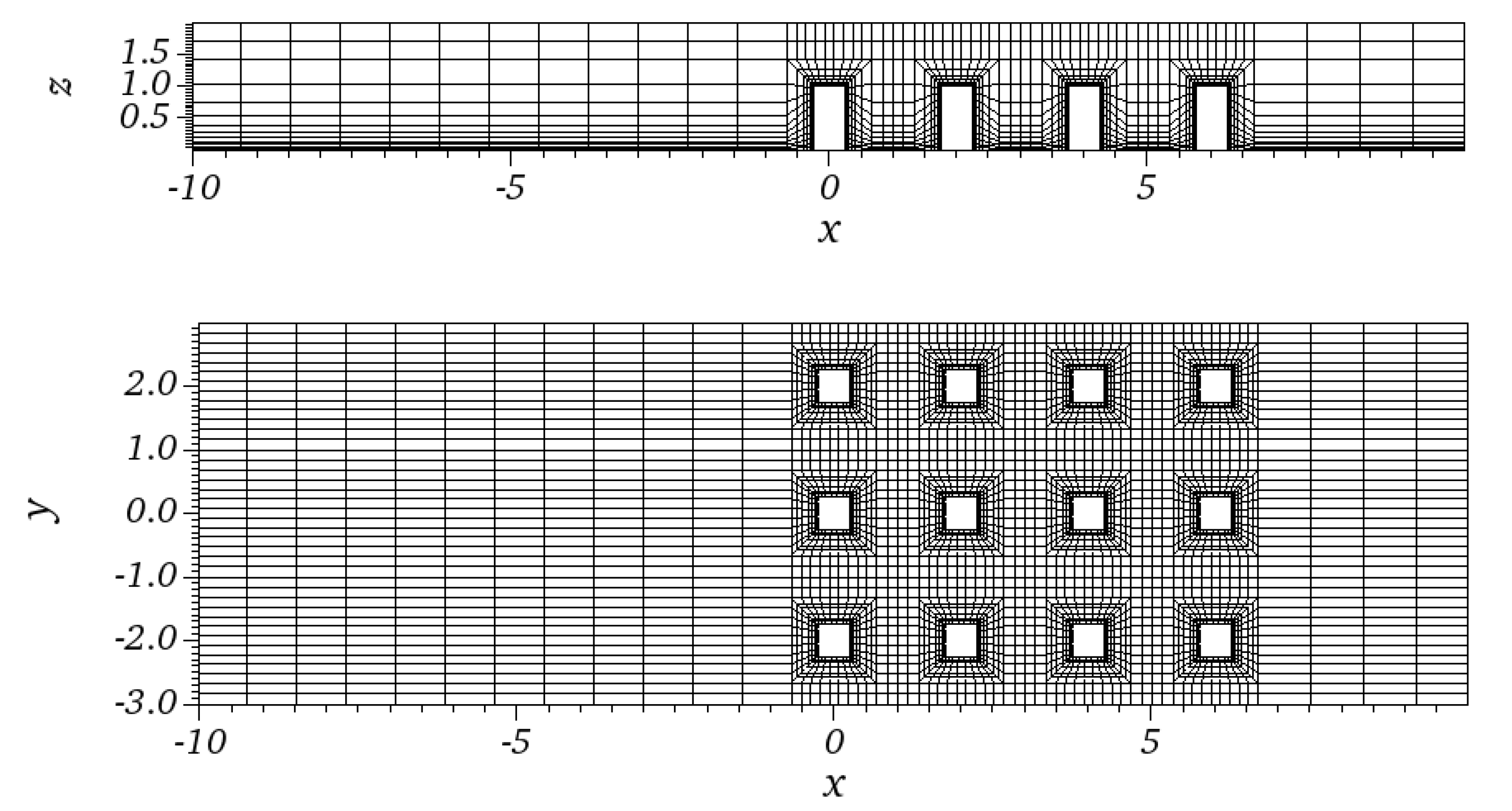
In the flow through an urban environment, disregarding the thermal and buoyancy effects, the compressible effects are expected to be small due to the relatively low velocities. A requirement for accurate simulations is the use of a numerical discretization which allows for an adequate representation of the complete range of scales of turbulence. The incompressible Navier–Stokes equations are described in the following, where $\mathbf{u}$ is the velocity vector, p the pressure, t the time and $\nu$ the kinematic viscosity.

$$\begin{array}{c}{\displaystyle \frac{\partial \mathbf{u}}{\partial t}+(\mathbf{u}·\nabla )\mathbf{u}=-\nabla p+\nu {\nabla }^2\mathbf{u}.}\hfill \\ \nabla ·\mathbf{u}=0.\hfill \end{array}$$

(2)

The well-resolved LES was performed using the open-source numerical code Nek5000 developed by Fischer et al. [10] at the Argonne National Laboratory and based on the spectral-element method (SEM) that is proposed by Patera [37]. In this code, the Galerkin approximation is used for the spatial discretization and third-order discretization in time is used with explicit extrapolation and implicit backward differentiation for the nonlinear and viscous terms, respectively. The SEM combines the geometrical flexibility required to discretize the urban geometry with the high-order accuracy of spectral methods. As discussed below, the geometry of the buildings and streets is discretized using hexahedral elements and the scale disparity of the turbulent flows is resolved using the Gauss–Lobatto–Legendre (GLL) quadrature within each element. The turbulent flow through the simplified urban environment simulated here is shown in Figure 1, where the level of detail in the instantaneous flow structures can be observed. Note that the length and velocity scales are the building height H and the freestream velocity $U_{\infty }$, respectively. The computational domain spans from $x=-10$ to 10 in the streamwise direction. In the wall-normal and spanwise directions, the computational domain spans from $y=0$ to 2 and from $z=-3$ to 3, respectively. The inflow is a laminar boundary layer at $R{e}_{{\delta }^{*}}=450$ (which is the Reynolds number based on displacement thickness) and a volume-force tripping is used to trigger the transition to turbulence as in Ref. [38]. We use the outflow condition developed by Dong et al. [39] and the top boundary has a zero-stress condition in the y direction together with a prescribed freestream velocity in x and zero velocity in z. Finally, periodic boundary conditions are imposed in the spanwise direction.

The well-resolved LES approach relies on a relaxation-term (RT) filter, which accounts for the contribution of the smallest unresolved turbulent scales through a dissipative force [41]. This force is given by $-\chi H_f\left(u\right)$, then it is added to the right-hand side of the momentum equation in (2) and it is defined by a high-pass spectral filter $H_f$ and a model parameter $\chi$. In these simulations, $H_f$ affects the two last modes and $\chi$ is set to 200 based on H and $U_{\infty }$. This technique was employed by Vinuesa et al. [42] to simulate the turbulent flow around a NACA4412 wing section up to a Reynolds number based on freestream velocity and chord length of $R{e}_c$ = 1,000,000. Note that this method was thoroughly validated in the context of the spectral-element method by Negi et al. [43] by comparing a fully-resolved direct numerical simulation of a turbulent wing at $R{e}_c$ = 400,000 with a well-resolved LES of the same flow case, achieving excellent statistical agreement. Around 90% of the turbulent kinetic energy is resolved by the LES and the subgrid-scale (SGS) model accounts for the remaining 10%. This is similar to what was documented by Bobke et al. [44] in the context of Fourier–Chebyshev methods and this will be the simulation approach adopted in this study. We would like to note that the role of this type of high-fidelity numerical simulation and of data-driven methods is becoming progressively more critical to tackle sustainability challenges, such as the development of more sustainable urban environments as explored in this work [45,46].

Mesh Design

The mesh design plays a critical role in the performance of a flow simulation. As discussed above, Nek5000 is based on the spectral-element method developed by Patera [37] and the considered mesh comprises a set of elements along with an eight-point GLL quadrature inserted in each of the elements. The elements are distributed uniformly in the domain with exception of the near-obstacle regions (where the element distribution is refined to provide additional resolution). Refinement is applied progressively in the wall-normal direction of the obstacles and depends upon an expansion rate that determines the level of refinement as well as the extent of the refined region. Figure 2 shows slices of the spectral-element mesh used for the flow simulation. The refinement ensures that the resolution is sufficient in the most relevant areas, i.e., the spaces between the obstacles. Note that this representation only shows the limits of the elements. Recall that within the elements, we have a GLL quadrature and thus the actual number of points is greater than what can be observed by inspecting Figure 2. We employed 70,000 elements to discretize the domain and a polynomial order $N=7$, which yields a total number of grid points of around 36 million. The criteria for mesh design approximately followed the guidelines by Negi et al. [43], who thoroughly validated them in the context of Nek5000 simulations of turbulent wings. In particular, these guidelines dictate that the inner-scaled mesh spacing in the turbulent boundary layer should satisfy $\Delta x^{+}<20$, $\Delta z^{+}<9$ and $\Delta y_w^{+}<1$. In the wakes of the obstacles, the guideline for mesh design is $h/\eta <9$, where h is the local cubic root of cell volume and $\eta$ is the Kolmogorov scale.

The meshing process relies on a meshing tool developed in the context of this project, which is based on a Swift parallel-computing scripting language as well as the Parsl parallel scripting library [47]. This tool allows the meshing process to be significantly more efficient, since the meshes can be created by defining a set of geometrical and resolution parameters. Furthermore, these tools make use of parallel-computing resources such that the mesh-building process is carried out efficiently.

3. Analysis of the Well-Resolved LES

The flow through an urban array is a multi-scale problem: one can describe different scales characterizing turbulent production and dissipation such as the wake layer above the obstacles and the urban canopy beneath it, with the shear layer and the different coherent vortical structures. The wake layer is the region of large-scale turbulence that is just above the mean height of the urban obstacles and is mostly the result of flow separation that occurs at the leading edge of the upstream blocks, whereas the shear layer is the region within the canopy level and on both sides of each urban obstacle. In the following, the mean streamwise component of the velocity at the building height is denoted by $U_H$ and $W_b$ denotes the building width. The Reynolds number of the flow, based on H and $U_{\infty }$, is 10,000. The numerical simulation exhibits an aspect ratio of the urban array of $0.67$, which implies that we do not expect the skimming-flow regime described by Oke [26] to be completely reached.

We first focus on the mean flow as well as its downstream evolution and then we will focus on the turbulent kinetic energy and the Reynolds stresses. The evolution of the turbulent characteristics of the flow as it goes through the urban array will also be investigated. Note that the turbulence statistics were calculated over an interval of 130 convective time units and we started collecting them 54 time units after the beginning of the simulation. This is conducted to ensure that the initial transients do not have an impact on the presented results. The criteria for convergence of turbulence statistics and the identification of initial transients have been defined based on the guidelines by Vinuesa et al. [48].

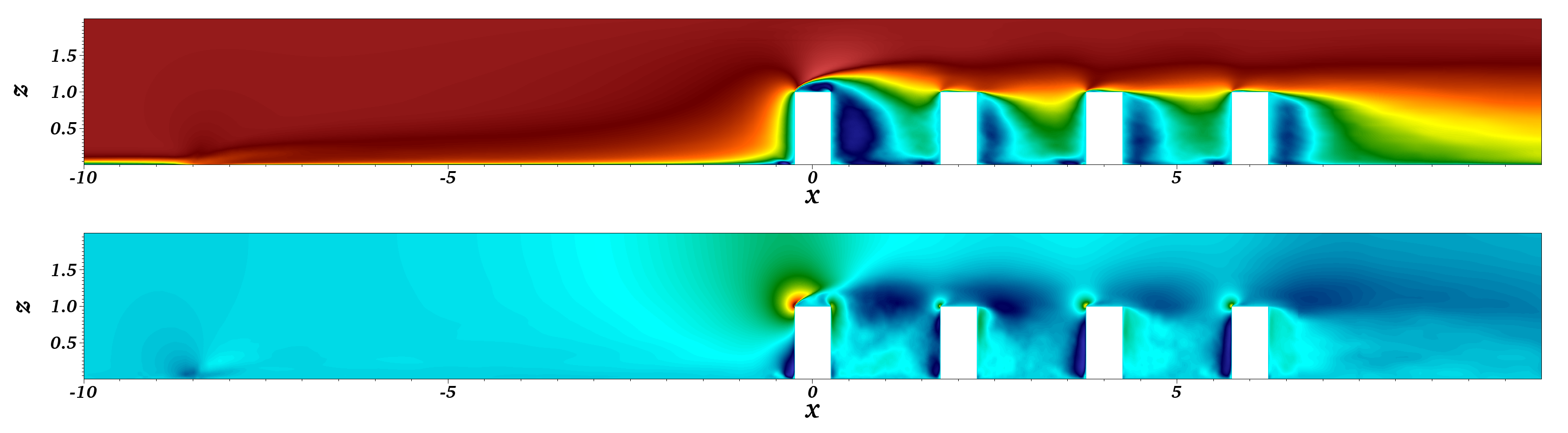
3.1. Analysis of the Mean Flow

The mean velocity components have been scaled by $U_{\infty }$. Figure 3 shows both the streamwise and the wall-normal mean velocity component of the flow in an $xz$-plane at the centerplane for the four streets. The non-dimensional streamwise component of the mean flow highlights three regions. Above the building height, at $z/H\simeq 1.4$, one can identify a high-speed region ($U/U_{\infty }\approx 1.1$). In this region, the influence of the urban obstacle is not visible at a local scale which is contrary to the region of the flow beneath the upper-roof level. Two regions can be identified for $z/H<1.3$: first, a thin shear layer ($0.8<z/H<1.2$) interacts with a strong wall-normal velocity gradient $\partial U/\partial z$. The canopy drag significantly slows down the flow as it enters the streets and it leads to regions of close-to-zero mean streamwise velocity, with a region of reversed flow close to the downstream side of each building. Close to the wall and the windward side of each building, there is a very small region of reversed flow which confirms the patterns described by Hwang and Yang [23]: A separation point in front of each cubical obstacle results in a small recirculation bubble. This pattern observed for a single obstacle is present in front of each building of the urban array. Despite the strong canopy drag force, the structure of the flow around each cubical obstacle of the array is very similar to that found around a single block, such as the reversed flow region that one can identify downstream of each building. On the other hand, some features of the flow around a cubical obstacle can only be identified in the first building. For example, one can observe a small area of reversed flow above the roof of the first obstacle, which confirms the presence of the roof vortex identified by Sousa [19]. This roof vortex is a direct consequence of the detachment of the boundary layer on the roof of the first obstacle and it leads to a wake-layer region in which the flow is separated and where turbulence is dominated by large and coherent eddies. These results provide an interesting parallelism with the behavior in wind farms, where beyond the third row of wind turbines the wake profiles become independent of the row and the lost energy is provided to the flow through vertical exchange.

The wall-normal mean velocity component, shown in Figure 3 (bottom), exhibits two regions for the four streets: an area of downward flow close to the downstream building and an area of upward flow near the upstream building. However, by analyzing the magnitude of the wall-normal velocity component, it can inferred that only a small fraction of the flow is going back down towards the street. There is also a small region of upward flow at the upstream corner of each obstacle (even if its intensity decreases considerably as one moves downstream). This region, along with the region of downward flow above each street ($1.2>z/H>0.8$), explains how the flow bypasses each urban obstacle. The fact that the region of downward flow mentioned above does not reach the near-wall region within the street is a direct consequence of the (approximate) skimming-flow regime presented here: The bulk of the flow from above the urban canopy does not enter the street canyons and therefore the flow from above the urban canopy does not interact with the flow from within the urban canopy. Globally, the urban-canopy drag decelerates the wind so that there is a mass flux upwards and away from the top of the canopy. Downwind the urban environment, there is an exit region similar to the one observed by Belcher et al. [15] in the case of forest canopies. This exit region, located between $6<x/H<8$, extends to a distance of order $2H$ downwind the urban environment where the mean flow suddenly increases because of the removal of the canopy drag.

Figure 4 exhibits the evolution of the mean streamwise velocity fields at two horizontal planes located at $z/H=0.85$ and $z/H=0.25$. As the angle of incidence of the flow is $0^{\circ }$, symmetric flow is observed as may be expected, with higher velocity within the street canyons. Streamwise velocity values are higher on both sides of the first urban obstacle and then decrease as one moves downstream. The freestream flow impacts the first urban obstacle with high streamwise velocity. Then, the flow around the cubical obstacle creates a wake in which the flow separates because of the detachment of the boundary layer from the surface of the obstacle. This results in an increased pressure-drag force. Regions of reversed flow ($U\approx -0.4$) on both sides of the first cubical obstacle indicate flow separation and they indicate the presence of the side vortices described by Sousa [19]. The flow impacting the other obstacles is, therefore, disturbed and turbulence is dominated by large and coherent eddies. However, a wake with separated flow downstream of each obstacle can be observed, which is also under the influence the previous obstacle wake. Closer to the wall, as shown in Figure 4 (bottom), the influence of the wall with lower streamwise velocity values can be observed. In the spanwise direction, a strong velocity gradient $\partial U/\partial y$ results in a non-dimensional streamwise velocity close to zero downstream each obstacle within the streets, with a large region of reversed flow. This region, together with the positive streamwise velocity on both sides, are indications of the presence and the location of the legs of the arch vortex.

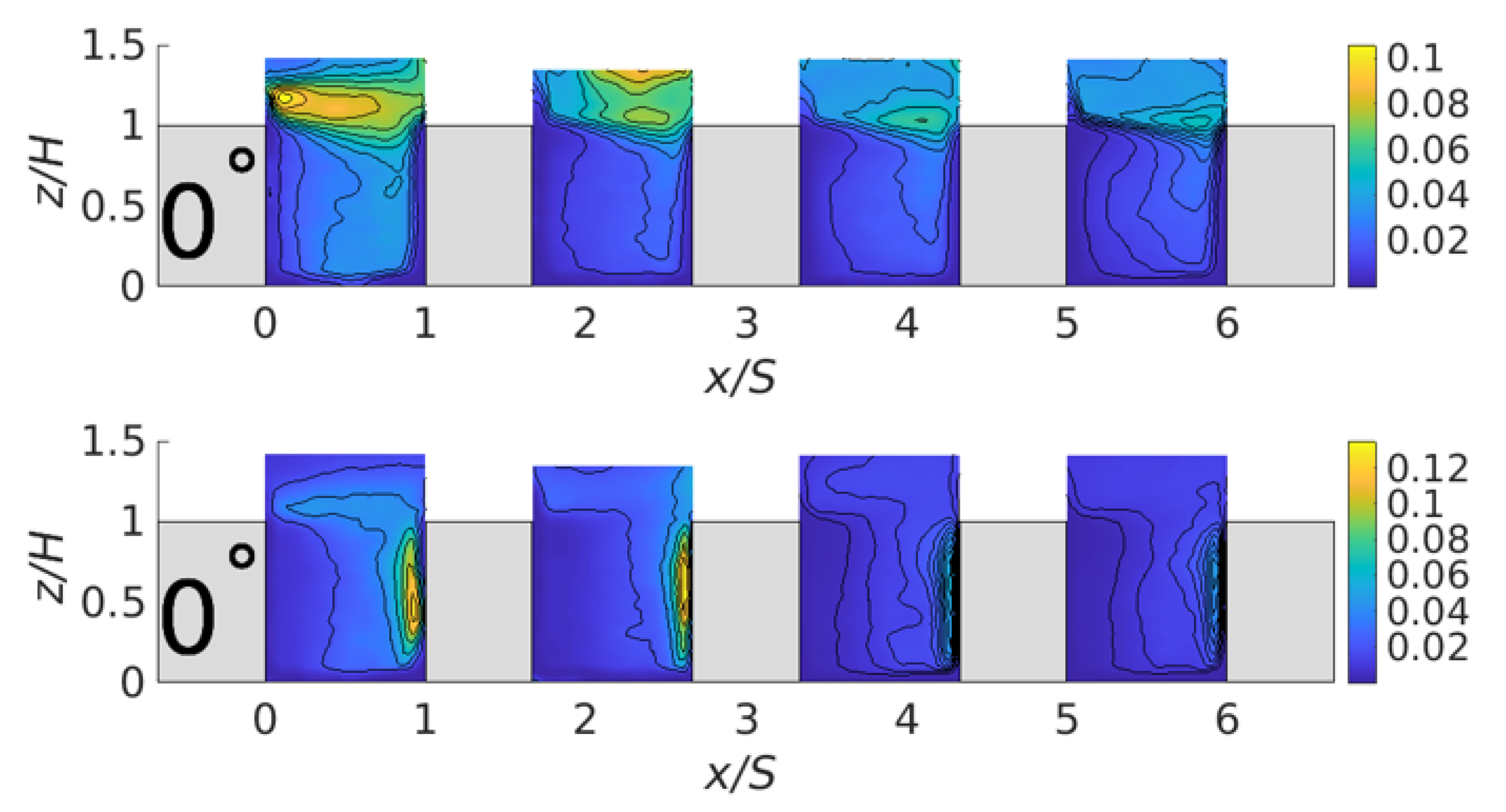
3.2. Analysis of the Turbulent Fluctuations

The root-mean squares (rms) of the turbulent fluctuations denoted by $u_{\mathrm{rms}}$ and $v_{\mathrm{rms}}$ in the streamwise and spanwise directions, respectively, are studied next. Note that $U_{inf}^2$ has been used to non-dimensionalize the turbulent fluctuations. Figure 5 exhibits the streamwise and the spanwise components of the turbulent fluctuations in a vertical plane at the urban array centerplane.

Figure 5 shows high levels of turbulence at the roof level in the first street and within the street at the upstream side of the downstream building. These high levels of turbulence suggest strong exchanges of fluid and scalar quantities between the streets and the mean flow above the urban array. Figure 5 also shows that the region of high turbulence at the upper-roof level is mainly due to the streamwise component of the velocity fluctuations, whereas, within the street, the turbulence is driven by the spanwise component. This notable energy exchange is related to the energy lost in overcoming the buildings, which is associated to the pressure drop between the windward and leeward sides of the obstacles. Note that this is in excellent agreement with the experimental results by Monnier et al. [9]. The wall-normal component (not shown) is not zero in those regions but is considerably weaker than the two other components. The strength of the separating shear layer near the upper-roof level decreases significantly from the first street to the following street as one moves downstream. Therefore, the exchanges of scalar quantities and fluid are considerably weaker between the urban canopy and the freestream above it. The presence of a canopy introduces new processes and, as described by Belcher et al. [15] in the case of forest canopies, turbulence is dissipated by a number of mechanisms. First, eddies of all scales work against the form drag of canopy elements. Turbulence is then transferred from larger eddies to the smallest scales and therefore quickly dissipated. Secondly, viscous dissipation is the second main process that dissipates turbulence. Figure 5 shows that, within the region where the flow adapts to the urban canopy, there are regions of high turbulence intensity, but as one moves downstream this turbulence is strongly damped through the canopy. In particular, the damping of $u_{\mathrm{rms}}^2$ is augmented by the return to isotropy and the turbulence hence evolves into an equilibrium form. The shear layer mentioned above develops at the canopy top where the coherent eddies also form and the exchanges of scalar quantities significantly dampen in the most downstream regions since the flow from above the canopy does not enter the streets. Note that the great wealth of data produced with high-fidelity simulations can help to develop robust data-driven tools to model certain aspects of the flow and to perform predictions of the complex flow behavior observed in urban areas [49,50].

4. Comparison with Experimental Data

Despite the difference of geometry between our urban array and the one used by Monnier et al. [9] for their experiments, as well as the differences in inflow conditions, it is possible perform some comparisons between the well-resolved LES and the stereoscopic PIV measurements. The aspect ratio of the urban array used by Monnier et al. [9] is over $0.67$, which mimics an urban environment with relatively high buildings compared with the street width. Therefore, contrary to what we expected from the numerical data, Monnier et al. [9] expected a skimming-flow regime to be reached. In Figure 6, we show mean streamwise velocity $U/U_H$ and the mean-wall normal velocity $W/U_H$ at $y/W_b=0$, where the data is extracted from the experimental campaign by Monnier et al. [9].

It is possible to observe very similar flow patterns in the experimental and the numerical databases. However, in the experimental data, the bulk of the flow from above the urban canopy does not enter the streets as is shown by the very low magnitude of the reversed flow observed in the streets, compared with the well-resolved LES. In particular, the region of negative wall-normal velocity on the windward side of the downstream building is of higher intensity in the LES. Therefore, a higher flow rate from above the urban canopy enters the streets when the streets are wider. The streamwise and spanwise velocity fluctuations, shown in Figure 7, confirm that a skimming flow is reached almost immediately, with high level of turbulence at the roof level but not in the streets. The main difference between the two databases can be observed in the first street: In the well-resolved LES, Figure 5 exhibits moderate levels of turbulence in the street, which is not the case in the experiments shown in Figure 7 (experiments). This synergistic use of simulations and experiments can help to address the limitations from both research, eventually resulting in more accurate flow data, for instance, through the development of pertinent corrections [51,52].

5. Summary and Conclusions

In this work we provide thorough analysis of the turbulent statistics of the flow through an urban array. A summary of the most relevant features is given below.

First of all, the effects of the urban canopy on the freestream high-speed incoming flow have been highlighted. Above the urban canopy and within the streets parallel to the flow, it is possible to identify regions of high-speed freestream flow. However, at the roof level and on each side of the urban obstacle, there are strong velocity gradients which mark the separating shear layer and results in regions of lower velocity. Regions of reversed flow have been highlighted and the well-resolved LES show the presence of coherent vortical structures such as the legs of the arch vortex.

Within the streets, the flow between two obstacles can be separated into two distinct regions: A region of reversed flow close to the leeward side of the upstream block and a region of higher velocity towards the windward side of the downstream block. The region of reversed flow exhibits low TKE whereas the other region shows higher levels of turbulence. The streamwise and the spanwise components of the velocity fluctuations are the main contributors to the TKE distribution and they clearly show how the flow bypasses each obstacle. High levels of turbulence have also been observed on each side of each cubical obstacle and at the upper-roof level, which are the result of the interaction between the freestream high-speed flow from above the urban canopy and the shear layers. This increased TKE, mainly due to the streamwise velocity fluctuations, is responsible for the formation of the arch vortex. Globally, the flow field exhibits a coherent structure of the flow within the urban canopy, reflected in the recirculation bubbles and regions of reversed flow. As one moves downstream, the flow reaches an equilibrium and the bulk of the flow from above does not interact with the flow from the streets. This is the case for the first street in the experiments where the streets are narrower: After a region in which the flow adapts to the canopy, a skimming-flow regime is reached and the exchange of scalar quantities and fluid between the urban canopy and the region above are not favored.

The mixing characteristics of the flow through an urban environment are significantly affected by its geometry. In an environment with narrow streets and relatively high buildings, as encountered in many American cities, the bulk of the flow from above the urban canopy does not interact with the flow within the streets. The skimming-flow regime is observed and consequently all the scalar quantities are trapped within the urban canopy and this can be an issue for pollutant dispersion. When the street width becomes wider, a larger fraction of the flow from above the canopy interacts with the flow from within it. Therefore, this is a more favorable situation when it comes to reducing pollutant concentration.

To conclude, a coherent picture of the flow field can be identified and the correlation between the geometry and the regime of the flow has been investigated. The influences of the geometry of the urban array on the turbulence statistics and therefore on the mixing characteristics of the flow have been studied. This directly impacts the transport of scalar quantities such as pollutants and the temperature. Additional extensions of this work could follow the work by Monnier et al. [9], who investigated the influence of the angle of incidence on the turbulence statistics and the vortical structures. Moreover, it would be relevant to investigate the flow through a complex urban environment, especially taking into account the geometry of the terrain where the city is built, as conducted by Belcher et al. [15] for the flow through a forest canopy.

References

1. Torres, P.; Le Clainche, S.; Vinuesa, R. On the experimental, numerical and data-driven methods to study urban flows. Energies 2021, 14, 1310. [Google Scholar] [CrossRef]
2. Britter, R.; Hanna, S. Flow and dispersion in urban areas. Annu. Rev. Fluid Mech. 2003, 35, 469–496. [Google Scholar] [CrossRef]
3. Stathopoulos, T. Pedestrian level winds and outdoor human comfort. J. Wind Eng. Ind. Aerodyn. 2006, 94, 769–780. [Google Scholar] [CrossRef]
4. Garbero, V.; Salizzoni, P.; Soulhac, L. Experimental study of pollutant dispersion within a network of streets. Bound.-Layer Meteorol. 2010, 136, 457–487. [Google Scholar] [CrossRef]
5. Belcher, S. Mixing and transport in urban areas. Philos. Trans. R. Soc. A Math. Phys. Eng. Sci. 2005, 363, 2947–2968. [Google Scholar] [CrossRef]
6. Baik, J.; Kim, J. A numerical study of flow and pollutant dispersion characteristics in urban street canyons. J. Appl. Meteorol. 1999, 38, 1576–1589. [Google Scholar] [CrossRef]
7. Vinuesa, R.; Schlatter, P.; Malm, J.; Mavriplis, C.; Henningson, D. Direct numerical simulation of the flow around a wall-mounted square cylinder under various inflow conditions. J. Turbul. 2015, 16, 555–587. [Google Scholar] [CrossRef]
8. Nagib, H.; Corke, T. Wind microclimate around buildings: Characteristics and control. J. Wind Eng. Ind. Aerodyn. 1984, 16, 1–15. [Google Scholar] [CrossRef]
9. Monnier, B.; Goudarzi, S.; Vinuesa, R.; Wark, C. Turbulent structure of a simplified urban fluid flow studied through stereoscopic particle image velocimetry. Bound.-Layer Meteorol. 2018, 166, 239–268. [Google Scholar] [CrossRef]
10. Fischer, P.F.; Lottes, J.W.; Kerkemeier, S.G. Nek5000: Open Source Spectral Element CFD Solver. 2008. Available online: https://nek5000.mcs.anl.gov (accessed on 12 July 2021).
11. Vinuesa, R.; Fick, L.; Negi, P.; Marin, O.; Merzari, E.; Schlatter, P. Turbulence Statistics in a Spectral Element Code: A Toolbox for High-Fidelity Simulations; Technical Report; Argonne National Lab (ANL): Argonne, IL, USA, 2017. [Google Scholar]
12. Kastner-Klein, P.; Rotach, M. Mean flow and turbulence characteristics in an urban roughness sublayer. Bound.-Layer Meteorol. 2004, 111, 55–84. [Google Scholar] [CrossRef]
13. Reynolds, R.; Castro, I. Measurements in an urban-type boundary layer. Exp. Fluids 2008, 45, 141–156. [Google Scholar] [CrossRef] [Green Version]
14. Finnigan, J. Turbulence in plant canopies. Annu. Rev. Fluid Mech. 2000, 32, 519–571. [Google Scholar] [CrossRef]
15. Belcher, S.; Harman, I.; Finnigan, J. The wind in the willows: Flows in forest canopies in complex terrain. Annu. Rev. Fluid Mech. 2012, 44, 479–504. [Google Scholar] [CrossRef]
16. Stull, R. Mean boundary layer characteristics. In An Introduction to Boundary Layer Meteorology; Springer: Berlin/Heidelberg, Germany, 1988; pp. 1–27. [Google Scholar]
17. Dupont, S.; Brunet, Y. Edge flow and canopy structure: A large-eddy simulation study. Bound.-Layer Meteorol. 2008, 126, 51–71. [Google Scholar] [CrossRef]
18. Liakos, A.; Malamataris, N. Direct numerical simulation of steady state, three dimensional, laminar flow around a wall mounted cube. Phys. Fluids 2014, 26, 053603. [Google Scholar] [CrossRef]
19. Sousa, J. Turbulent flow around a surface-mounted obstacle using 2D-3C DPIV. Exp. Fluids 2002, 33, 854–862. [Google Scholar] [CrossRef]
20. Hussein, H.; Martinuzzi, R. Energy balance for turbulent flow around a surface mounted cube placed in a channel. Phys. Fluids 1996, 8, 764–780. [Google Scholar] [CrossRef]
21. Becker, S.; Lienhart, H.; Durst, F. Flow around three-dimensional obstacles in boundary layers. J. Wind Eng. Ind. Aerodyn. 2002, 90, 265–279. [Google Scholar] [CrossRef]
22. Monnier, B.; Neiswander, B.; Wark, C. Stereoscopic particle image velocimetry measurements in an urban-type boundary layer: Insight into flow regimes and incidence angle effect. Bound.-Layer Meteorol. 2010, 135, 243–268. [Google Scholar] [CrossRef]
23. Hwang, J.; Yang, K. Numerical study of vortical structures around a wall-mounted cubic obstacle in channel flow. Phys. Fluids 2004, 16, 2382–2394. [Google Scholar] [CrossRef] [Green Version]
24. Schenk, F.; Vinuesa, R. Enhanced large-scale atmospheric flow interaction with ice sheets at high model resolution. Results Eng. 2019, 3, 100030. [Google Scholar] [CrossRef]
25. Martinuzzi, R.; Havel, B. Turbulent flow around two interfering surface-mounted cubic obstacles in tandem arrangement. J. Fluids Eng. 2000, 122, 24–31. [Google Scholar] [CrossRef]
26. Oke, T. Street design and urban canopy layer climate. Energy Build. 1988, 11, 103–113. [Google Scholar] [CrossRef]
27. Coceal, O.; Thomas, T.; Castro, I.; Belcher, S. Mean flow and turbulence statistics over groups of urban-like cubical obstacles. Bound.-Layer Meteorol. 2006, 121, 491–519. [Google Scholar] [CrossRef]
28. Xing, F.; Mohotti, D.; Chauhan, K.A. Experimental and numerical study on mean pressure distributions around an isolated gable roof building with and without openings. Build. Environ. 2018, 132, 30–44. [Google Scholar] [CrossRef]
29. Fernando, H.; Zajic, D.; Di Sabatino, S.; Dimitrova, R.; Hedquist, B.; Dallman, A. Flow, turbulence, and pollutant dispersion in urban environments. Phys. Fluid 2010, 22, 051301. [Google Scholar] [CrossRef]
30. Pol, S.; Brown, M. Flow patterns at the ends of a street canyon: Measurements from the Joint Urban 2003 field experiment. J. Appl. Meteorol. Climatol. 2008, 47, 1413–1426. [Google Scholar] [CrossRef] [Green Version]
31. Hamlyn, D.; Britter, R. A numerical study of the flow field and exchange processes within a canopy of urban-type roughness. Atmos. Environ. 2005, 39, 3243–3254. [Google Scholar] [CrossRef]
32. Assimakopoulos, V.; Georgakis, C.; Santamouris, M. Experimental validation of a computational fluid dynamics code to predict the wind speed in street canyons for passive cooling purposes. Sol. Energy 2006, 80, 423–434. [Google Scholar] [CrossRef]
33. Jones, W.; Launder, B.E. The prediction of laminarization with a two-equation model of turbulence. Int. J. Heat Mass Transf. 1972, 15, 301–314. [Google Scholar] [CrossRef]
34. Yamartino, R.; Wiegand, G. Development and evaluation of simple models for the flow, turbulence and pollutant concentration fields within an urban street canyon. Atmos. Environ. (1967) 1986, 20, 2137–2156. [Google Scholar] [CrossRef]
35. Boddy, J.; Smalley, R.; Dixon, N.; Tate, J.; Tomlin, A. The spatial variability in concentrations of a traffic-related pollutant in two street canyons in York, UK—Part I: The influence of background winds. Atmos. Environ. 2005, 39, 3147–3161. [Google Scholar] [CrossRef]
36. Louka, P.; Belcher, S.; Harrison, R. Modified street canyon flow. J. Wind Eng. Ind. Aerodyn. 1998, 74, 485–493. [Google Scholar] [CrossRef]
37. Patera, A. A spectral element method for fluid dynamics: Laminar flow in a channel expansion. J. Comput. Phys. 1984, 54, 468–488. [Google Scholar] [CrossRef]
38. Vinuesa, R.; Hosseini, S.; Hanifi, A.; Henningson, D.; Schlatter, P. Pressure-gradient turbulent boundary layers developing around a wing section. Flow Turbul. Combust. 2017, 99, 613–641. [Google Scholar] [CrossRef] [Green Version]
39. Dong, S.; Karniadakis, G.; Chryssostomidis, C. A robust and accurate outflow boundary condition for incompressible flow simulations on severely-truncated unbounded domains. J. Comput. Phys. 2014, 261, 83–105. [Google Scholar] [CrossRef]
40. Jeong, J.; Hussain, F. On the identification of a vortex. J. Fluid Mech. 1995, 285, 69–94. [Google Scholar] [CrossRef]
41. Schlatter, P.; Stolz, S.; Kleiser, L. LES of transitional flows using the approximate deconvolution model. Int. J. Heat Fluid Flow 2004, 25, 549–558. [Google Scholar]
42. Vinuesa, R.; Negi, P.S.; Atzori, M.; Hanifi, A.; Henningson, D.S.; Schlatter, P. Turbulent boundary layers around wing sections up to Rec = 1,000,000. Int. J. Heat Fluid Flow 2018, 72, 86–99. [Google Scholar] [CrossRef] [Green Version]
43. Negi, P.S.; Vinuesa, R.; Hanifi, A.; Schlatter, P.; Henningson, D.S. Unsteady aerodynamic effects in small-amplitude pitch oscillations of an airfoil. Int. J. Heat Fluid Flow 2018, 71, 378–391. [Google Scholar] [CrossRef] [Green Version]
44. Bobke, A.; Vinuesa, R.; Örlü, R.; Schlatter, P. History effects and near-equilibrium in adverse-pressure-gradient turbulent boundary layers. J. Fluid Mech. 2017, 820, 667–692. [Google Scholar] [CrossRef]
45. Vinuesa, R.; Azizpour, H.; Leite, I.; Balaam, M.; Dignum, V.; Domisch, S.; Felländer, A.; Langhans, S.D.; Tegmark, M.; Fuso Nerini, F. The role of artificial intelligence in achieving the Sustainable Development Goals. Nat. Commun. 2020, 11, 233. [Google Scholar] [CrossRef] [PubMed] [Green Version]
46. Gupta, S.; Langhans, S.D.; Domisch, S.; Fuso-Nerini, F.; Felländer, A.; Battaglini, M.; Tegmark, M.; Vinuesa, R. Assessing whether artificial intelligence is an enabler or an inhibitor of sustainability at indicator level. Transp. Eng. 2021, 4, 100064. [Google Scholar] [CrossRef]
47. Torres, P. High-Order Spectral Simulations of the Flow in a Simplified Urban Environment. Bachelor’s Thesis, Polytechnic University of Valencia, Valencia, Spain, 2020. [Google Scholar]
48. Vinuesa, R.; Prus, C.; Schlatter, P.; Nagib, H. Convergence of numerical simulations of turbulent wall-bounded flows and mean cross-flow structure of rectangular ducts. Meccanica 2016, 51, 3025–3042. [Google Scholar] [CrossRef] [Green Version]
49. Srinivasan, P.A.; Guastoni, L.; Azizpour, H.; Schlatter, P.; Vinuesa, R. Predictions of turbulent shear flows using deep neural networks. Phys. Rev. Fluids 2019, 4, 054603. [Google Scholar] [CrossRef] [Green Version]
50. Guastoni, L.; Güemes, A.; Ianiro, A.; Discetti, S.; Schlatter, P.; Azizpour, H.; Vinuesa, R. Convolutional-network models to predict wall-bounded turbulence from wall quantities. arXiv 2020, arXiv:2006.12483. [Google Scholar]
51. Vinuesa, R.; Schlatter, P.; Nagib, H.M. Role of data uncertainties in identifying the logarithmic region of turbulent boundary layers. Exp. Fluids 2014, 55, 1751. [Google Scholar] [CrossRef]
52. Vinuesa, R.; Nagib, H.M. Enhancing the accuracy of measurement techniques in high Reynolds number turbulent boundary layers for more representative comparison to their canonical representations. Eur. J. Mech.-B/Fluids 2016, 55, 300–312. [Google Scholar] [CrossRef]
Figure 1. Instantaneous visualization of the flow under study showing vortical structures identified with the λ 2 method [40]. The shown isosurface is 50 (scaled with the freestream velocity and the obstacle height) and the structures are colored in terms of the streamwise velocity from (dark blue) 1 to (dark red) 1.8.
Applsci 11 06472 g001
Figure 2. Slices of the spectral-element mesh: (top) slice at z = 0 and (bottom) slice at y = 0.1 (where the lengths are scaled with the building height). Note that the GLL points within elements are not shown.
Applsci 11 06472 g002
Figure 3. (Top) Mean streamwise velocity U, where colors range from (dark blue) 0.4 to (dark red) 1.1. (Bottom) Mean wall-normal velocity W, with colors ranging from (dark blue) 0.35 to (dark red) 1. The y = 0 plane is shown.
Applsci 11 06472 g003
Figure 4. Mean streamwise velocity U on the (top) z = 0.85 and (bottom) z = 0.25 planes, where colors range from (dark blue) 0.4 to (dark red) 1.1.
Applsci 11 06472 g004
Figure 5. (Top) Streamwise normal Reynolds stress u rms 2 , where colors range from (dark blue) 0 to (dark red) 0.2. (Bottom) Square of the rms spanwise velocity fluctuations v rms 2 , where colors range from (dark blue) 0 to (dark red) 0.25. The y = 0 plane is shown.
Applsci 11 06472 g005
Figure 6. (Top) Non-dimensional mean streamwise velocity U / U H and (bottom) mean wall-normal velocity W / U H at y / W b = 0 . Data extracted from the experiments by Monnier et al. [9]. Note that S denotes street separation.
Applsci 11 06472 g006
Figure 7. (Top) Square of the root-mean-squared velocity fluctuations (top) u rms 2 / U H 2 and (bottom) v rms 2 / U H 2 at y / W b = 0 . Data extracted from the experiments by Monnier et al. [9]. Note that S denotes street separation.
Applsci 11 06472 g007
Publisher’s Note: MDPI stays neutral with regard to jurisdictional claims in published maps and institutional affiliations.