Abstract
The objective of this study was to determine the influence of vehicular traffic on the environmental noise levels of the Santa Marta City tourist route on the Colombian coast. An analysis of vehicle types and frequencies at various times of the day over nearly a year helped to track the main sources of environmental noise pollution. Five sampling points were selected, which were distributed over 12 km, with three classified as peripheral urban and two as suburban. The average traffic flow was 966 vehicles/h and was mainly composed of automobiles, with higher values in the peripheral urban area. The noise level was 103.3 dBA, with background and peak levels of 87.2 and 107.3 dBA, respectively. The noise level was higher during the day; however, there were no differences between weekdays and weekends. The results from the analysis of variance showed that the number of vehicles and the noise levels varied greatly according to the time of day and sampling point location. The peak and mean noise levels were correlated with the number of automobiles, buses and heavy vehicles. The mean noise levels were similar at all sample points despite the traffic flow varying, and the background noise was only correlated for automobiles (which varied much more than the heavy vehicles between day and night).
1. Introduction
Among the different anthropogenic activities associated with noise sources, emissions from vehicular traffic greatly exceed the background noise levels of cities. Therefore, traffic is the main source of acoustic pollution, contributing to approximately 80% of total environmental noise [1,2]. In recent years, noise pollution associated with road traffic has become one of the main environmental problems in urban spaces. Studies conducted in the US, Europe, China, and Latin America observed high levels of noise, with values ranging between 50 and 88 dBA [3,4,5,6,7,8]. These levels have been increasing due to the growth of personal vehicles as a consequence of urban expansion and issues related to public transportation [9,10,11]. The current situation is worsening due to inappropriate driver behavior, such as the overuse of horns or powerful sound equipment [12,13].
It is estimated that, globally, around 60 million people are exposed to high levels of noise [14], which has led to great concern as noise is a stressor with repercussions to physiological and psychological health. Physiological effects include respiratory alterations [15], digestive disorders [16,17], and cardiovascular disorders [15,18,19], while psychological effects include fatigue, irritability, anxiety, lack of confidence, and burnout syndrome [20], which increase the likelihood of committing mistakes and exposing workers to the risk of accidents, reducing their productivity and increasing the economic costs invested in medical services and treatment [21,22].
Recent studies on the harmful effect of noise on health observed the impact on sleep quality. The immediate effects on sleep stages such as waking and wakefulness resulted in drowsiness, impaired cognitive function, low daytime performance, and long-term, chronic sleep disorders [20]. Children and elderly adults are the most vulnerable to this [23,24,25,26]. In general, we can establish the effects of noise on sleep from 30 dBA, interference of oral communication from 35 dBA, cardiovascular effects between 65 and 70 dBA, and the gradual loss of hearing with continuous exposure to noise levels over 85 dBA [27], and a brief exposure to sound levels exceeding 120 dBA without hearing protection may even cause physical pain [28].
Aside from the impact on public health, noise also results in negative economic impacts, where properties exposed to high noise levels lose an equivalent of between 0.23% and 1.6% of their price with every increase of 1 dBA of noise over 55 dBA [29,30]. In addition, a direct relationship between devaluation and increasing road traffic has been demonstrated [31]. Noise has also affected the hotel industry, as people prefer to stay in hotels with low exposure to noise, even if staying in such hotels is more expensive [21].
The high levels of noise (above 75 dBA) reported in Colombian cities (Bogotá, Medellín, Cali, Bucaramanga, and San Juan de Pasto) were attributed to road traffic [32], specifically from taxis, cars, and buses. The noise levels also exceed the national Colombian limit (for more detail about the Colombian noise limit, see Table S1 in Supplementary Materials) [33,34,35,36].
Each road vehicle generates a particular amount of noise, which can be grouped into two generic types: (1) noise caused by mechanics, called engine noise, whis is associated with the movement of pistons, combustion processes, the cooling system, valves, gearbox transmissions, the exhaust pipe, and vibrations of the bodywork [37], and (2) noise generated by displacement, which can be divided into rolling noise, which is the product of friction between the tires and the pavement, and aerodynamic noise, which results from interactions between the bodywork and the air [38]. Therefore, road traffic noise depends on the volume and composition of traffic flow, as well as vehicle velocities and the type of road surface, among other factors [39].
Santa Marta is a coastal city in the Colombian Caribbean whose main activity is tourism, as indicated by the extensive development of the hotel sector close to the “Ruta del Sol” tourist route, which received 517,917 people in 2012 [40]. The “Ruta del Sol” is an important highway, enabling fluid transport of supplies for Santa Marta. For that reason, in 2010, the road upgraded its infrastructure to become a highway that could deal with high traffic flow, but unfortunately, this subsequently led to an increase in environmental noise. Hence, this study seeks to determine the levels of environmental noise and its relationship with vehicular flow as a source of noise, in addition to establishing whether the noise caused by traffic depends on the number of vehicles or rather on the composition of the vehicular flow.
Five sampling points were selected, distributed over 12 km: three classified as peripheral urban and two as suburban. The number and type of vehicles were recorded in addition to measuring the average, minimum, maximum, background, and peak noise twice daily (day and night) during the week and on weekends. The results were analyzed using analysis of variance (ANOVA), and the influence of road traffic and noise was performed using Pearson’s correlation. The acoustic sampling was carried out at a height of 4 m, thus integrating the propagation of the noise in the field (with five different orientations of the microphone).
2. Materials and Methods
2.1. Study Area
The study area was located in one of the most important hotel sectors of the city of Santa Marta, which is located to the south of the city and contains an important section of the Ruta del Sol (Transversal del Caribe) or Route 90 of the national road network. A 12-km section of the highway from just after the “Ye de Gaira” heavy traffic diversion road until the border of the urban area of the city was chosen as the study area. The highway has two lanes in each direction separated by a median strip (Figure 1) allowing a vehicle running speed between 80 and 100 km/h [41].
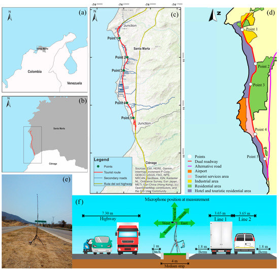
Figure 1.
General global position of the study area (a), zoomed-in image of the study area (b), map of the main road studied and major junctions (c), map of the road and surrounding land use (d), photograph of the monitoring campaign at point 5 (e), and diagram of a transverse section at a sampling point (f).
A total of 5 sampling points were distributed equidistantly approximately every 2 km (Figure 1). The first 3 sampling points were in the peri-urban area (1–3), with a medium population density and a high number of hotels. The last two in the suburban area (4 and 5) had low population densities and fewer hotels, but the hotels were of a higher category (offering better comfort and services). It is important to mention that in this section of the road, there are fewer heavy vehicles; however, sampling point 5 was close to the junction with the alternative heavy goods route.
2.2. Traffic Flow Characterization
The vehicle flow count was performed manually for a period of 70 min, starting 5 min before the 1-h noise sampling period and ending 5 min after it (Figure 2). The vehicles were classified into 4 categories: automobiles, buses, trucks, and motorcycles. Vehicle counts were carried out during two periods of the day, daytime (from 7:01 a.m. to 9:00 p.m.) and night-time (from 9:01 p.m. to 7:00+1 a.m.), classified according to two different types of days of the week; weekdays (Monday–Friday) and weekends (Saturday, Sunday and holidays). In total, six samples were taken during the day and two at night during each day of the sampling period. The monitoring was carried out between 17 July 2014 and 27 March 2015 according to the availability of staff and equipment.

Figure 2.
Time scale of noise and traffic flow measurement along with the orientation and state of the microphones.
2.3. Environmental Noise Measurement
The noise measurement was carried out in accordance with the Colombian standard (Annex 3 Chapter II, resolution 627/2006) that is consistent with ISO 1996 [42]. A 7-min sample was taken in each of the directions of the microphone (north (N), south (S), east €, west (W), and vertical (V)). Each position was sampled for 7 min in such a way that the 5 samples were uniformly distributed during 1 h of sampling (Figure 2). The hourly value was calculated using Equation (1), where is the acoustic parameter and N, S, W, E, and V are for each of the five microphone positions during the 1 h of sampling:
The sampling was carried out in the median strip central vial separator at a height of 4 m using a type 1 sonometer (Casella model CEL-633-C1K1). The equipment configuration was run in fast mode (sampling data every 100 ms) with an A weighting filter. The selected acoustic parameters were as follows: equivalent continuous level (LAeq, to establish the noise level), maximum (LAmax) and minimum (LAmin), the percentiles as indicators of the peak noise level (LA5 and LA10) of the road traffic, the mean value (LA50) to contrast with LAeq, and the background noise level (LA90 and LA95). The hourly value per parameter was calculated using Equation (1).
2.4. Data Analysis and Statistical Processing
Analysis of variance (ANOVA) with a significance level of 95% (a = 0.05) was carried out to determine the influence of the experimental parameters (time of day and day of the week) on the variation of traffic flow and noise levels at the sampling points [43]. Likewise, hierarchical ANOVA was performed (a = 0.05) in order to determine which experimental factors (position, time of day, and day of the week) better explained the possible variation of the noise results [44,45,46]. Finally, a Pearson test was developed to determine the possible correlation between the vehicle types and acoustic parameters.
3. Results
3.1. Traffic Flow Characterization
The results showed an abundance of automobiles (57%), followed by motorcycles (24%), buses (14%), and trucks (5%), with cars and motorcycles showing a considerable variation across the sampling points. The largest numbers of vehicles were observed at sampling point 2, but also at sampling point 5 during the night on weekends (Figure 3). In general, there was more traffic in the daytime than at night, but at night, greater variation was observed between the sampling points. There were more cars during the day (66%) compared with at night, as was also noted for the other types of vehicles, but with less variation between day and night (Figure 3). Furthermore, a higher number of trucks and fewer buses were observed on weekdays. In general, weekday traffic exceeded that of weekends by 50%, except for buses.
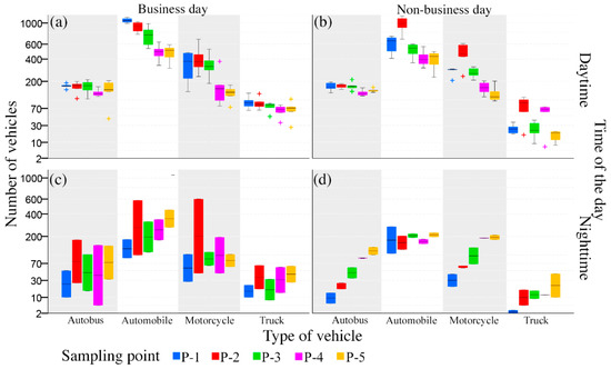
Figure 3.
Quantity of vehicle types recorded per day of the week, time of day, and sampling point (P: point). (a) Weekday, daytime. (b) Weekend, daytime. (c) Weekday, night-time. (d) Weekend, night-time.
3.2. Environmental Noise
Figure 4 shows the results of the equivalent, maximum, and minimum noise levels. The equivalent noise (LAeq) values were similar at all sampling points; during the daytime, the difference between the points was around 2 dBA on both weekdays and weekends, while night-time showed a greater variation of 7 dBA on weekdays and 5 dBA on weekends. The sampling locations were similar throughout the week, except for point 1 in the daytime and point 5 at night (see Supplementary Materials). In addition, the noise levels were higher during the day than at night, especially at sampling points 1, 2, and 3, while less variation was observed at sampling points 4 and 5 (Table S2, Supplementary Materials).
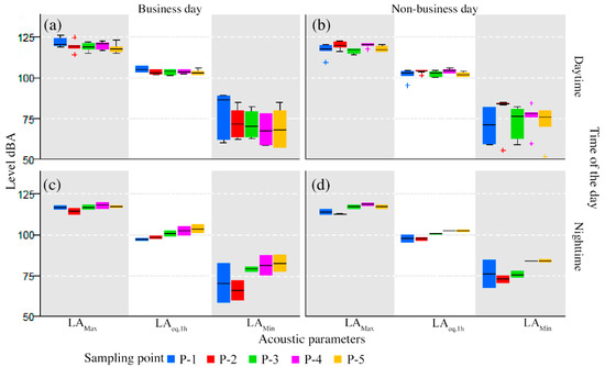
Figure 4.
Equivalent, maximum, and minimum noise levels on each day of the week, time of day, and sampling point. (a) Weekday, daytime. (b) Weekend, daytime. (c) Weekday, night-time. (d) Weekend, night-time.
The LAmax values exhibited similar behavior to those of LAeq, but with a slightly greater amplitude between the maximum and minimum values (Figure 4), where the daytime values reached 3.6 dBA on both weekdays and weekends, and the night-time values reached 3.8 dBA on weekdays and 6.0 dBA at weekends (Table S2, Supplementary Materials). Similarly, slightly higher values with greater variability were reported during the day than at night, with very little difference to be noted between day and night. Hence, the behavior of LAmax was more similar to that of LAeq, despite its increased variability (Figure 4). The LAmin values exhibited greater variability. Therefore, there was a greater difference in the values measured at the different sampling points of up to 7 dBA between the maximum and minimum (Table S2, Supplementary Materials). Hence, the behavior of the time of day and day of the week was opposite to that seen for the previous parameters, showing high values at night (sampling points 2, 3, and 4) and on weekends (sampling points 3, 4, and 5).
LA50 exhibited similar results to those of LAeq but with a slight increase (Figure 5). The same behavior was exhibited for the time of day and day of the week but with even greater variation. The background noise exhibited substantial variation between the different times of the day, with higher values recorded during the day than at night, especially at sampling points 1 and 2. This was similar to the day of the week variable, with higher values recorded on weekdays than on weekends and sampling points 1 and 5 exhibiting a greater difference (Figure 5). Finally, the peak values exhibited the least variation between the experimental design variables (time of the day and day of the week). However, the behavior was similar to that of LAeq or LA50, excluding the records taken at sampling point 5 during the night and sampling points 2 and 4 on weekends (Figure 5). More detail about the data is available in Table S3 in Supplementary Materials.
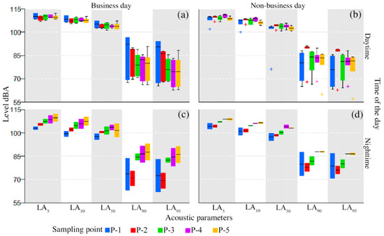
Figure 5.
Acoustic indicators (percentiles) for each day of the week, time of day and sampling point. (a) Weekday, daytime. (b) Weekend, daytime. (c) Weekday, night-time. (d) Weekend, night-time.
3.3. Statistical Analysis
3.3.1. Analysis of Variance
The variation in the number of vehicles was influenced by the time of day (ANOVA p-value 0.000) and the sampling points (p-value 0.003). Additionally, when discriminating by vehicle type, the day of the week also influenced the variation of the quantity of vehicles (p-value 0.000 in all types). If the results were tested by the sampling points, a significant influence was observed for automobiles (p-value 0.000) and motorcycles (p-value 0.000). In addition, the test considering the day of the week produced significant results for trucks (p-value 0.000) and automobiles (p-value 0.042). More details are in Supplementary Materials Table S4.
The environmental noise ANOVA test showed that there was no significant difference between noise levels (Figure 6), presenting one homogeneous group (p-value 0.410), with sampling point 1 exhibiting the greatest variation in noise values and sampling points 4 and 5 exhibiting the lowest.
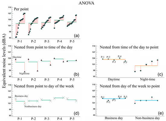
Figure 6.
ANOVA graphs for the equivalent noise level with different nested sampling factors (P. sampling point). (a) The environmental noise ANOVA test. (b) ANOVA nested from sampling points to time of the day for noise level values. (c) ANOVA nested from the time of day to sampling points for noise level values. (d) ANOVA nested from sampling points to the day of the week for noise level values. (e) ANOVA nested from the day of the week to sampling points for noise level values. The hourly mean of LAeq is represented by ■, ▲ represents the mean of LAeq per time of the day, ● represents the mean of LAeq per sampling point, and ✕ represents the mean of LAeq per type of day of the week. The green line is the mean of LAeq. The orange line is the mean of five sampling points for day or night. The blue line is the mean of five sampling points for each type of day.
The time of day showed a statistically significant influence on the noise values reported at the sampling points (Figure 6). The average level was greater during the day, except at sampling point 5, but there was higher variability above the average level at night. Consequently, Figure 6c shows that during the day, the noise level showed a less significant difference between the sampling points, while the night-time measurements showed a more significant difference, corroborating that there was high variability in the nocturnal data. Finally, there was also no significant difference in the noise levels between the sampling points, depending on the day of the week; however, they were slightly higher on weekdays in some cases (Figure 6). The nested ANOVA shows that the days of the week had no influence on the variability of the noise levels; however, at sampling point 2 on weekdays and sampling points 1 and 4 on weekends, a non-significant difference was observed (Figure 6).
3.3.2. Pearson Correlation Test
According to the ANOVA results, there was a correlation between the hours of the day (which impacted the noise level) and the type of vehicle. The selected acoustic parameters were the mean, maximum, minimum, peak, and background values. In the daytime hours, there was a relationship between the peak, LAmax, and equivalent noise levels for trucks and between the peak, LAeq, and background values for automobiles. In the night-time, buses influenced the peak, maximum, and LAeq noise levels, while automobiles and trucks only influenced the peak and LAeq (Figure 7). In all cases, the correlation was positive, showing the direct correlation between the number of vehicles and increasing environmental noise levels. In general, automobiles and trucks showed the greater number of correlations with the acoustic parameters during the daytime, while buses showed greater correlation at night, followed by automobiles and trucks. Finally, the peak, maximum, and continuous equivalent noise were the parameters most influenced by the quantity of vehicles, while the minimum and background levels were not influenced, except in one case where automobiles and LA90 appeared to be linked. More details are in Supplementary Materials Table S5.
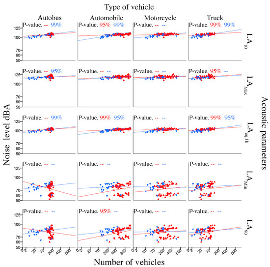
Figure 7.
Pearson correlation coefficient between acoustic parameters and vehicle type (Sig.: significance grade,
▲: day, and
▼: night).
4. Discussion
The results show that the peri-urban area (sampling points 1, 2, and 3) had different behavior from the suburban sampling points (sampling points 4 and 5). This may be because there were more commercial and tourist activities in the peri-urban area. This is consistent with a study of high traffic in the urban area of Motilla de Palancar (Spain), which decreased with the distance from the urban limit [47]. Likewise, the vehicular flow was similar to other studies with road infrastructures similar to that of this study, reporting international scale flows between 700 and 1145 vehicles/h [48] and a range of 725–973 vehicles/h on a national scale [49]. The latter is very similar to this study, with a predominance of cars (70%), followed by buses (16%), motorcycles (13%), and trucks (1%). The results show a similarity in the predominant type of vehicle that is consistent with both international studies [48] as well as national studies [34]. The latter reference is very similar to this work, where there was a predominance of cars (70%), followed by buses (16%), motorcycles (13%), and trucks (1%).
The results also show that the traffic flow increased from the night to the day (61.9%). Automobiles constituted the largest proportion of traffic (65.9%), followed by trucks (62.3%). These values were greater than those observed in Belgrade (Serbia), with general values of 52.3%, 58.3% for automobiles, and 51.9% for trucks [50]. The differences in traffic flow at different times of the day may be due to the working period of the day (mainly daytime), increasing the numbers of automobiles and buses due to their high demand. The variation between weekdays and weekends exhibited a decrease in all categories on weekends, except at sampling point 5 for trucks. This result is in accordance with a study in New York (US), where the number of trucks significantly decreased on weekends while the number of automobiles and buses increased [3].
The reported noise levels were 10 and 20 dBA greater than those observed in previous studies [3,51,52,53,54]. Here, LAmin reached the average LAeq of previous studies [33,55,56,57,58,59]. Therefore, the results show that the environmental noise level was very high in the sampling area. The other studies were conducted in urban areas with different flow patterns and mainly considered speed circulation, observing low truck flow and driving rhythms affected by traffic signaling. These flow pattern properties did not occur along the Ruta del Sol route, which exhibited continuous flow (without congestion) and a higher speed limit (80–100 km/h). The results for Mexico confirmed the results of this analysis, which exhibited a high noise level in the suburban area of a city, where the speed limit is greater [60]. Similarly, a study on noise level and speed circulation observed an exponential relationship between these two factors, where an increase in speed resulted in a higher increase in the noise level [61,62].
However, the noise values can also be influenced by the monitoring protocol. The first difference is the location of the sound level meter in relation to the road (central road separator). Normally, there is a meter located on one side of the road. The second is the height of the microphone from the ground, which is usually 1.5 m, but Colombian law requires a height of 4 m, which affects the acoustic properties [63]. Finally, Harris [64] stated that the continuous noise equivalent (LAeq) is an adequate indicator of road traffic noise. It is also sensitive to isolated events with high noise levels, such as low traffic flow with high speed, which could have caused the increment in the noise levels observed in the present results.
Although the results of studies in Ireland [65] and Medellín [57] disagree with the present results, their noise levels and vehicle flows exhibited a decreasing trend from the day to the night, as observed here. The ANOVA test showed similar results, with a significant difference between the median noise level and vehicle flows during the day and night. The day/night ratio of 2.6 dBA obtained here is similar to the results observed in New York and Nagpur (India), with day/night ratios of 2.4 and 1.9 dBA, respectively. These studies also observed a decrease in vehicle flows from the day to the night [3,13]. Therefore, it can be inferred that vehicle flow is the main source of environmental noise, because an increase in the number of vehicles also increased the noise level.
The great difference between the day and night noise levels at the first three sampling points (close to the urban area) can be explained by much less public and personal transport from the surrounding areas at night, while the minor differences observed at sampling points 4 and 5 could be due to the continuous flow, especially of trucks, throughout the day and night.
The total traffic flow, number of motorcycles and buses, and the equivalent noise level did not differ between weekdays and weekends. This is similar to the results observed in New York [3], where the reported noise levels did not vary between the days of the week.
The ANOVA test confirmed that the mean noise level was similar at all sample points; however, the traffic flow was not. Therefore, the sampling points and reported noise levels did not show a relationship with the traffic flow. However, the ANOVA test exhibited homogeneity between buses and trucks, thereby confirming a relationship between these vehicle categories and the equivalent continuous noise. This was confirmed by the Pearson test, with a direct relationship between LAeq and the buses or trucks. The present results are similar to those of other national studies in Bogota and Tunja, Colombia, which observed a correlation between LAeq and automobiles, buses, and trucks [34,52], and international studies conducted in Belgium, which observed a relationship between trucks and the noise level [58].
The results of the Pearson test also show that LA10 was correlated with the trucks, buses, and automobiles, which may be because trucks release six times the amount of sound energy produced by automobiles [66]. Therefore, trucks tend to exhibit a greater influence on the maximum recorded levels. This can also be observed for buses but not for automobiles. However, a high quantity of vehicles can produce a comparable amount of noise to one truck, as the ratios of noise produced by vehicles are 10 automobiles per 1 truck and 4 automobiles per 1 bus [67]. These ratios were established according to the noise emission levels of each type of vehicle measured in Santiago de Chile, with trucks producing mean noise emissions of 101.4 dBA under 30 km/h, which could increase to 106.5 dBA at speeds above 60 km/h [68].
Finally, the correlation test showed that the background noise was only correlated for automobiles, which can be explained by the high variability in traffic flow along with the cessation of urban and suburban activities at night. This again indicates that the flow of vehicles in the study area significantly influenced the environmental noise levels observed in this study, which decreased during the night when there was a low flow of vehicles. Another reason for the lack of correlation of vehicles with LAmin and LA90 could be due to the kind of noise created at high speeds, where aerodynamic noise is prevalent. This type the noise is associated with high frequencies [69], so their air field propagation capacity is low and can be influenced more by the Doppler effect. Hence, establishing a speed limit could be a solution. However, studies have shown that the impact of speed on reducing environmental noise is not significant [70,71].
The high flow of automobiles (the most common type) observed with fewer buses and trucks influenced the environmental noise in the study area, leading to high values despite the deviation of heavy traffic from this route. However, it is necessary to carry out complementary noise measurements in areas close to the hotels to confirm that the level of noise emission from the road is impacting the buildings before proposing physical noise mitigation measures such as acoustic barriers.
Supplementary Materials
The following are available online at https://www.mdpi.com/article/10.3390/app11167196/s1, Table S1: Maximum permissible standards of environmental noise levels, expressed in decibels dBA, Table S2: Mean of Equivalent continuous noise level (LAeq), maximum (LAmax) and minimum LAmin) on each time of day, day of the week and sampling point in the Santa Marta tourist route, Table S3: Mean of noise level percentiles for each time of day, day of the week and sampling point in the Santa Marta tourist route, Table S4: P-values of ANOVA test of the traffic flow characterisation, Table S4. Coefficient of correlation between type of vehicle and acoustic parameter, Table S5: Coefficient of correlation between type of vehicle and acoustic parameter
Author Contributions
Conceptualization, D.A.J.-U., D.D. and A.M.V.-P.; methodology, D.A.J.-U., D.D. and A.M.V.-P.; validation, D.A.J.-U., D.D. and A.M.V.-P.; formal analysis, D.A.J.-U., D.D., Z.L.F. and A.M.V.-P.; data curation, D.A.J.-U., D.D. and A.M.V.-P.; writing—original draft preparation, D.A.J.-U. and A.M.V.-P.; writing—review and editing, D.A.J.-U., D.D., Z.L.F. and A.M.V.-P. All authors have read and agreed to the published version of the manuscript.
Funding
This research received no external funding. The article processing charges were funded by Centro de Investigación en Ecosistemas de la Patagonia (CIEP).
Institutional Review Board Statement
Not applicable.
Informed Consent Statement
Not applicable.
Data Availability Statement
Data available on request.
Acknowledgments
Thanks to Universidad del Magdalena for the support received.
Conflicts of Interest
The authors declare no conflict of interest.
References
- Branbilla, G. Physical assessment and rating of urban noise. In Environmental Urban Noise; WIT Press: Southampton, UK, 2001; pp. 15–61. [Google Scholar]
- Lebiedowska, B. Acoustic Background and Transport Noise in Urbanised Areas: A Note on the Relative Classification of the City Soundscape. Transp. Res. Part D Transp. Environ. 2005, 10, 341–345. [Google Scholar] [CrossRef]
- Ross, Z.; Kheirbek, I.; Clougherty, J.E.; Ito, K.; Matte, T.; Markowitz, S.; Eisl, H. Noise, Air Pollutants and Traffic: Continuous Measurement and Correlation at a High-Traffic Location in New York City. Environ. Res. 2011, 111, 1054–1063. [Google Scholar] [CrossRef]
- Nugent, C.; Blanes, N.; Fons, J.; Sáinz de la Maza, M.; Ramos, M.; Domingues, F.; van Beek, A.; Houthuijs, D. Noise in Europe 2014; EEA Report; European Environment Agency: Luxembourg, 2014; p. 2014. [Google Scholar]
- Mavrin, V.; Makarova, I.; Prikhodko, A. Assessment of the Influence of the Noise Level of Road Transport on the State of the Environment. Transp. Res. Procedia 2018, 36, 514–519. [Google Scholar] [CrossRef]
- Bravo-Moncayo, L.; Chávez, M.; Puyana, V.; Lucio-Naranjo, J.; Garzón, C.; Pavón-García, I. A Cost-Effective Approach to the Evaluation of Traffic Noise Exposure in the City of Quito, Ecuador. Case Stud. Transp. Policy 2019, 7, 128–137. [Google Scholar] [CrossRef]
- Wallas, A.E.; Eriksson, C.; Bonamy, A.-K.E.; Gruzieva, O.; Kull, I.; Ögren, M.; Pyko, A.; Sjöström, M.; Pershagen, G. Traffic Noise and Other Determinants of Blood Pressure in Adolescence. Int. J. Hyg. Environ. Health 2019, 222, 824–830. [Google Scholar] [CrossRef]
- Wen, X.; Lu, G.; Lv, K.; Jin, M.; Shi, X.; Lu, F.; Zhao, D. Impacts of Traffic Noise on Roadside Secondary Schools in a Prototype Large Chinese City. Appl. Acoust. 2019, 151, 153–163. [Google Scholar] [CrossRef]
- Vogiatzis, K. Strategic Environmental Noise Mapping & Action Plans in Athens Ring Road (Atiiki Odos)—Greece. WSEAS Trans. Environ. Dev. 2011, 7, 315–324. [Google Scholar]
- Ögren, M.; Molnár, P.; Barregard, L. Road Traffic Noise Abatement Scenarios in Gothenburg 2015—2035. Environ. Res. 2018, 164, 516–521. [Google Scholar] [CrossRef]
- Hou, Q.; Leng, J.; Ma, G.; Liu, W.; Cheng, Y. An Adaptive Hybrid Model for Short-Term Urban Traffic Flow Prediction. Phys. A Stat. Mech. Its Appl. 2019, 527, 121065. [Google Scholar] [CrossRef]
- Calvo, J.A.; Álvarez-Caldas, C.; San Román, J.L.; Cobo, P. Influence of Vehicle Driving Parameters on the Noise Caused by Passenger Cars in Urban Traffic. Transp. Res. Part D Transp. Environ. 2012, 17, 509–513. [Google Scholar] [CrossRef]
- Vijay, R.; Sharma, A.; Chakrabarti, T.; Gupta, R. Assessment of Honking Impact on Traffic Noise in Urban Traffic Environment of Nagpur, India. J. Environ. Health Sci. Eng. 2015, 13, 1–10. [Google Scholar] [CrossRef]
- Murphy, E.; King, E. Environmental Noise Pollution: Noise Mapping, Public Health, and Policy; Elsevier: Amsterdam, The Netherlands, 2014; ISBN 978-0-12-411614-6. [Google Scholar]
- Recio, A.; Linares, C.; Banegas, J.R.; Díaz, J. The Short-Term Association of Road Traffic Noise with Cardiovascular, Respiratory, and Diabetes-Related Mortality. Environ. Res. 2016, 150, 383–390. [Google Scholar] [CrossRef] [PubMed]
- Zhang, L.; Gong, J.T.; Zhang, H.Q.; Song, Q.H.; Xu, G.H.; Cai, L.; Tang, X.D.; Zhang, H.F.; Liu, F.-E.; Jia, Z.S.; et al. Melatonin Attenuates Noise Stress-Induced Gastrointestinal Motility Disorder and Gastric Stress Ulcer: Role of Gastrointestinal Hormones and Oxidative Stress in Rats. J. Neurogastroenterol. Motil. 2015, 21, 189–199. [Google Scholar] [CrossRef]
- Wang, F.; Song, X.; Li, F.; Bai, Y.; Han, L.; Zhang, H.; Zhang, F.; Luo, X.; Shen, H.; Zhu, B. Occupational Noise Exposure and Hypertension: A Case-Control Study. J. Public Health Emerg. 2018, 2, 1–7. [Google Scholar] [CrossRef]
- Héritier, H.; Vienneau, D.; Foraster, M.; Eze, I.C.; Schaffner, E.; Thiesse, L.; Ruzdik, F.; Habermacher, M.; Köpfli, M.; Pieren, R.; et al. Diurnal Variability of Transportation Noise Exposure and Cardiovascular Mortality: A Nationwide Cohort Study from Switzerland. Int. J. Hyg. Environ. Health 2018, 221, 556–563. [Google Scholar] [CrossRef]
- Recio, A.; Linares, C.; Díaz, J. System Dynamics for Predicting the Impact of Traffic Noise on Cardiovascular Mortality in Madrid. Environ. Res. 2018, 167, 499–505. [Google Scholar] [CrossRef]
- WHO—World Health Organization. Environmental Noise Guidelines for the European Region; WHO Regional Office for Europe: Copenhagen, Denmark, 2018; ISBN 978-92-890-5356-3. [Google Scholar]
- Del Solar, L.M.; Gallegos, W.L.A.; Salinas, M.A.M. Síndrome de burnout en conductores de transporte público de la ciudad de Arequipa. Rev. Peru. Psicol. Trab. Soc. 2017, 2, 111–122. [Google Scholar]
- Garrido-Galindo, A.P.; Camargo Caicedo, Y.; Vélez-Pereira, A.M. Nivel Continuo Equivalente de Ruido En La Unidad de Cuidado Intensivo Neonatal Asociado al Síndrome de Burnout. Enferm. Intensiva 2015, 26, 92–100. [Google Scholar] [CrossRef]
- Öhrström, E.; Hadzibajramovic, E.; Holmes, M.; Svensson, H. Effects of Road Traffic Noise on Sleep: Studies on Children and Adults. J. Environ. Psychol. 2006, 26, 116–126. [Google Scholar] [CrossRef]
- Fyhri, A.; Aasvang, G.M. Noise, Sleep and Poor Health: Modeling the Relationship between Road Traffic Noise and Cardiovascular Problems. Sci. Total Environ. 2010, 408, 4935–4942. [Google Scholar] [CrossRef] [PubMed]
- Kim, M.; Chang, S.I.; Seong, J.C.; Holt, J.B.; Park, T.H.; Ko, J.H.; Croft, J.B. Road Traffic Noise: Annoyance, Sleep Disturbance, and Public Health Implications. Am. J. Prev. Med. 2012, 43, 353–360. [Google Scholar] [CrossRef] [PubMed]
- Paiva, K.M.; Cardoso, M.R.A.; Zannin, P.H.T. Exposure to Road Traffic Noise: Annoyance, Perception and Associated Factors among Brazil’s Adult Population. Sci. Total Environ. 2019, 650, 978–986. [Google Scholar] [CrossRef] [PubMed]
- Toronto Public Health. Health Effects of Noise; City of Toronto Community and Neighbourhood Services Toronto Public Health Health Promotion and Environment Protection Office: Toronto, ON, Canada, 2000; p. 20. [Google Scholar]
- Chepesiuk, R. Decibel Hell: The Effects of Living in a Noisy World. Environ. Health Perspect. 2005, 113, A34–A41. [Google Scholar] [CrossRef]
- Rubio Alférez, J.; Vanhooreweder, B.; Segués, F.; Kärkkäinen, A.; Giannopoulou, E.; Bellucci, P.; Report Best Practice in Strategic Noise Mapping. CEDR Conference of European Directors of Roads. 2013, p. 36. Available online: http://www.carreteros.org/explotacion/cedr/1_CEDR_august_2013.pdf (accessed on 27 July 2021).
- Istamto, T.; Houthuijs, D.; Lebret, E. Willingness to Pay to Avoid Health Risks from Road-Traffic-Related Air Pollution and Noise across Five Countries. Sci. Total Environ. 2014, 497–498, 420–429. [Google Scholar] [CrossRef]
- Von Graevenitz, K. The Amenity Cost of Road Noise. J. Environ. Econ. Manag. 2018, 90, 1–22. [Google Scholar] [CrossRef]
- Ideam, S.D.E.A. Meteorología, y Estudios Ambientales Documento Soporte Ruido Norma de Ruido Ambiental; IDEAM: Bogotá, Colombia, 2006; p. 268. [Google Scholar]
- Rendón, J.G.; Gómez, J.R.M.; Pardo, A.F.V.; Monsalve, R.A.A. Índices de ruido urbano en el día sin carro en la ciudad de Medellín. Rev. Faculdad Ing. USBMED 2010, 1, 78–85. [Google Scholar] [CrossRef]
- Ramírez González, A.; Domínguez Calle, E.A.; Borrero Marulanda, I. El Ruido Vehicular Urbano y Su Relación Con Medidas de Restricción Del Flujo de Automóviles. Rev. Acad. Colomb. Cienc. Exactas Físicas Nat. 2011, 35, 143–156. [Google Scholar]
- Quintero, J.R.G. Tendencias Actuales En El Estudio y Análisis Del Ruido Producido Por El Tráfico Rodado En Las Ciudades. Intekhnia 2012, 7, 173–192. [Google Scholar]
- Quintero, J.R.G. El ruido del tráfico vehicular y sus efectos en el entorno urbano y la salud humana. Puente 2013, 7. [Google Scholar] [CrossRef]
- Parrondo, J.L.; Velarde, S.; González, J.; Ballesteros, R.; Santolaria, C. Ruido de máquinas y vehículos. In Acústica Ambiental; Universidad de Oviedo: Asturias, Spain, 2006; pp. 123–140. ISBN 978-84-8317-531-6. [Google Scholar]
- Domingo, R.B. Ruido de tráfico. In Acústica Medioambiental; Editorial Club Universitario: San Vicente, Spain, 2010; Volume 1, pp. 233–246. ISBN 978-84-9948-020-6. [Google Scholar]
- Can, A.; Aumond, P. Estimation of Road Traffic Noise Emissions: The Influence of Speed and Acceleration. Transp. Res. Part D Transp. Environ. 2018, 58, 155–171. [Google Scholar] [CrossRef]
- MCIT—Ministerio de Comercio, Industria y Turismo, Perfil Económico de Magdalena. 2013. Available online: http://portalterritorial.gov.co/apc-aa-files/7515a587f637c2c66d45f01f9c4f315c/oee__magdalena_agosto_2013.pdf (accessed on 17 August 2015).
- Secretaria de Infraestructura Víal Departamento del Magdalena Elaboración Del Análisis, Estudio de Factibilidad Para La Liquidación, Distribución y Cobro de La Contribución de Valorización de Primera Fase Del Plan Vial Del Norte Del Departamento Del Magdalena. 2007. Available online: http://www.msv.ada.co/descargas/Informe_final_Sta_Marta.pdf (accessed on 14 December 2014).
- Ministerio de Ambiente, Vivienda y Desarrollo Territorial. Resolución 627 de 2006 por la cual se establece la norma nacional de emisión de ruido y ruido ambiental; Ministerio de Ambiente, Vivienda y Desarrollo Territorial: Bogotá, Colombia, 2006; p. 29. [Google Scholar]
- Garrido-Galindo, A.P.; Camargo Caicedo, Y.; Vélez-Pereira, A.M. Nivel de Ruido En La Unidad de Cuidado Intensivo Adulto: Medición, Estándares Internacionales e Implicancias Sanitarias. Univ. Salud 2015, 17, 163–169. [Google Scholar] [CrossRef][Green Version]
- Vélez-Pereira, A.M.; Camargo, Y. Aerobacterias Staphylococcus sp. en las Unidades de Cuidados Intensivos de un hospital universitario. Rev. Trauma 2012, 23, 183–190. [Google Scholar]
- Vélez-Pereira, A.M.; Camargo, Y. Aerobacterias en las unidades de cuidado intensivo del Hospital Universitario “Fernando Troconis”, Colombia. Rev. Cuba. Salud Pública 2014, 40, 362–368. [Google Scholar]
- Vélez-Pereira, A.M.; Camargo, Y. Análisis de los factores ambientales y ocupacionales en la concentración de aerobacterias en unidades de cuidado intensivo del Hospital Universitario Fernando Troconis, 2009 Santa Marta-Colombia. Rev. Cuid. 2014, 5, 595–605. [Google Scholar] [CrossRef]
- Ramis, J.; Alba, J.; García, D.; Hernández, F. Noise Effects of Reducing Traffic Flow through a Spanish City. Appl. Acoust. 2003, 64, 343–364. [Google Scholar] [CrossRef]
- Paviotti, M.; Vogiatzis, K. On the Outdoor Annoyance from Scooter and Motorbike Noise in the Urban Environment. Sci. Total Environ. 2012, 430, 223–230. [Google Scholar] [CrossRef]
- Duque, M.A.R.; Ladino, E.V. Modelación Matemática del Ruido Producido por el Tráfico en Seis Puntos Ubicados en la Ciudad de Pereira. Bachelor’s Thesis, Universidad Nacional de Colombia, Manizales, Colombia, 2007. [Google Scholar]
- Jakovljevic, B.; Paunovic, K.; Belojevic, G. Road-Traffic Noise and Factors Influencing Noise Annoyance in an Urban Population. Environ. Int. 2009, 35, 552–556. [Google Scholar] [CrossRef]
- Echeverry, Z.; Lucía, C. Un Aporte a La Gestión Del Ruido Urbano En Colombia, Caso de Estudio Municipio de Envigado. Master’s Thesis, Universidad Nacional de Colombia, Manizales, Colombia, 2010. [Google Scholar]
- Quintero González, J.R. Caracterización del ruido producido por el tráfico vehicular en el centro de la ciudad de Tunja, Colombia. Rev. Virtual Univ. Católica Norte 2012, 1, 311–343. [Google Scholar]
- Suthanaya, P.A. Modelling Road Traffic Noise for Collector Road (Case Study of Denpasar City). Procedia Eng. 2015, 125, 467–473. [Google Scholar] [CrossRef]
- Oyedepo, S.O.; Adeyemi, G.A.; Fayomi, O.S.I.; Fagbemi, O.K.; Solomon, R.; Adekeye, T.; Babalola, O.P.; Akinyemi, M.L.; Olawole, O.C.; Joel, E.S.; et al. Dataset on Noise Level Measurement in Ota Metropolis, Nigeria. Data Brief 2019, 22, 762–770. [Google Scholar] [CrossRef] [PubMed]
- López Redondo, L.L. Análisis del Aporte al Ruido Ambiental Emitido por los Vehículos Particulares en Bogotá. Engineering’s Thesis, Universidad de San Buenaventura, Bogotá, Colombia, 2007. [Google Scholar]
- Pacheco, J.; Franco, J.F.; Behrentz, E. Caracterización de los niveles de contaminación auditiva en Bogotá: Estudio piloto. Rev. Ing. 2009, 30, 72–80. [Google Scholar] [CrossRef]
- Yepes, D.L.; Gómez, M.; Sánchez, L.; Jaramillo, A. Metodología de Elaboración de Mapas Acústicos Como Herramienta de Gestión Del Ruido Urbano-Caso Medellín. Dyna 2009, 76, 29–40. [Google Scholar]
- Can, A.; Rademaker, M.; Van Renterghem, T.; Mishra, V.; Van Poppel, M.; Touhafi, A.; Theunis, J.; De Baets, B.; Botteldooren, D. Correlation Analysis of Noise and Ultrafine Particle Counts in a Street Canyon. Sci. Total Environ. 2011, 409, 564–572. [Google Scholar] [CrossRef]
- Casas-García, O.; Betancur-Vargas, C.M.; Montaño-Erazo, J.S. Revisión de la normatividad para el ruido acústico en Colombia y su aplicación. Entramado 2017, 11, 264–286. [Google Scholar] [CrossRef]
- Ibarra, D.; Ramírez-Mendoza, R.; López, E. Noise Emission from Alternative Fuel Vehicles: Study Case. Appl. Acoust. 2017, 118, 58–65. [Google Scholar] [CrossRef]
- Bravo, T.; Ibarra, D.; Cobo, P. Far-Field Extrapolation of Maximum Noise Levels Produced by Individual Vehicles. Appl. Acoust. 2013, 74, 1463–1472. [Google Scholar] [CrossRef]
- Winroth, J.; Kropp, W.; Hoever, C.; Beckenbauer, T.; Männel, M. Investigating Generation Mechanisms of Tyre/Road Noise by Speed Exponent Analysis. Appl. Acoust. 2017, 115, 101–108. [Google Scholar] [CrossRef]
- Jaramillo, A.; González, A.; Betancur, C.; Correa, M. Estudio Comparativo Entre Las Mediciones de Ruido Ambiental Urbano a 1,5 m y 4 m de Altura Sobre El Nivel Del Piso En La Ciudad de Medellín, Antioquia—Colombia. DYNA 2009, 76, 71–79. [Google Scholar]
- Harris, C.M. Manual de Medidas Acústicas y Control Del Ruido, 3rd ed.; McGraw-Hil: Madrid, Spain, 1995; Volume 1, ISBN 84-481-1619-4. [Google Scholar]
- O’Malley, V.; King, E.; Kenny, L.; Dilworth, C. Assessing Methodologies for Calculating Road Traffic Noise Levels in Ireland—Converting CRTN Indicators to the EU Indicators (Lden, Lnight). Appl. Acoust. 2009, 70, 284–296. [Google Scholar] [CrossRef]
- Sandoval, A.M. Ruido Por Tráfico Urbano: Conceptos, Medidas Descriptivas y Valoración Económica. Econ. Adm. 2005, 2, 1–49. [Google Scholar]
- Calixto, A.; Diniz, F.B.; Zannin, P.H.T. The Statistical Modeling of Road Traffic Noise in an Urban Setting. Cities 2003, 20, 23–29. [Google Scholar] [CrossRef]
- Platzer, U.; Iñiguez, R.; Cevo, J.; Ayala, F. Medición de Los Niveles de Ruido Ambiental En La Ciudad de Santiago de Chile. Rev. Otorrinolaringol. Cir. Cabeza Cuello 2007, 67, 122–128. [Google Scholar] [CrossRef]
- Jiménez-Uribe, D.A.; Daniels, D.; González-Álvarez, Á.; Vélez-Pereira, A.M. Influence of Vehicular Traffic on Environmental Noise Spectrum in the Tourist Route of Santa Marta City. Energy Rep. 2020, 6, 818–824. [Google Scholar] [CrossRef]
- Bohatkiewicz, J. Noise Control Plans in Cities—Selected Issues and Necessary Changes in Approach to Measures and Methods of Protection. Transp. Res. Procedia 2016, 14, 2744–2753. [Google Scholar] [CrossRef]
- Bunn, F.; Zannin, P.H.T. Urban Planning-Simulation of Noise Control Measures. Noise Control Eng. J. 2015, 63, 1–10. [Google Scholar] [CrossRef]


Publisher’s Note: MDPI stays neutral with regard to jurisdictional claims in published maps and institutional affiliations. |
© 2021 by the authors. Licensee MDPI, Basel, Switzerland. This article is an open access article distributed under the terms and conditions of the Creative Commons Attribution (CC BY) license (https://creativecommons.org/licenses/by/4.0/).