Methods for Noise Event Detection and Assessment of the Sonic Environment by the Harmonica Index

Abstract

Noise annoyance depends not only on sound energy, but also on other features, such as those in its spectrum (e.g., low frequency and/or tonal components), and, over time, amplitude fluctuations, such as those observed in road, rail, or aircraft noise passages. The larger these fluctuations, the more annoying a sound is generally perceived. Many algorithms have been implemented to quantify these fluctuations and identify noise events, either by looking at transients in the sound level time history, such as exceedances above a fixed or time adaptive threshold, or focusing on the hearing perception process of such events. In this paper, four criteria to detect sound were applied to the acoustic monitoring data collected in two urban areas, namely Andorra la Vella, Principality of Andorra, and Milan, Italy. At each site, the 1 s A-weighted short L_Aeq,1s time history, 10 min long, was available for each hour from 8:00 a.m. to 7:00 p.m. The resulting 92-time histories cover a reasonable range of urban environmental noise time patterns. The considered criteria to detect noise events are based on: (i) noise levels exceeding by +3 dB the continuous equivalent level L_AeqT referred to the measurement time (T), criteria used in the definition of the Intermittency Ratio (IR) to detect noise events; (ii) noise levels exceeding by +3 dB the running continuous equivalent noise level; (iii) noise levels exceeding by +10 dB the 50th noise level percentile; (iv) progressive positive increments of noise levels greater than 10 dB from the event start time. Algorithms (iii) and (iv) appear suitable for notice-event detection; that is, those that (for their features) are clearly perceived and potentially annoy exposed people. The noise events detected by the above four algorithms were also evaluated by the available anomalous noise event detection (ANED) procedure to classify them as produced by road traffic noise or something else. Moreover, the assessment of the sonic environment by the Harmonica index was correlated with the single event level (SEL) of each event detected by the four algorithms. The threshold value of 8 for the Harmonica index, separating the “noisy” from the “very noisy” environments, corresponds to lower SEL levels for notice-events as identified by (iii) and (iv) algorithms (about 88–89 dB(A)) against those identified by (i) and (ii) criteria (92 dB(A)).

1. Introduction

Urbanization is expected to continue in the future, causing an increase in both the number of people living in cities and the spatial densities of different noise sources. The noises in urban areas are composed of several sources (e.g., technological and anthropic sources), most of them masking natural sounds (e.g., geophonic and biophonic sounds), throughout the day. Among the abovementioned sources, road traffic noise is often predominant in urban areas, since it is widespread throughout space and time, impacting the people who are exposed to it. There is clear evidence in the literature that noise causes adverse effects on the health and well-being of citizens, e.g., sleep disturbance, annoyances, and cardiovascular diseases [1,2,3].

Because of this trend, many efforts have been implemented to mitigate noise impact and its harmful effects, as recommended by the environmental noise directive (END) 2002/49/EC) on the assessment and management of environmental noise [4]. Noise mapping of main sources (transport and industries) is one END requirement; its reporting to the European Commission is mandatory at least every five years. Noise maps represent—in a graphical way, through colored scale intervals—the spatial distributions of specific sound metrics, usually long-term averaged values such as day–evening–night level L_den in dB(A) introduced by the END [4]. They are primarily obtained by numerical models of outdoor sound propagation; many efforts were made in recent years, in Europe, to harmonize these models [5]. The role of sound measurements is, therefore, rather limited, even if it is important to tune the model to the real environmental setting. We should note that these measurements require appropriate instrumentation and trained technicians to perform them, are time consuming and expensive, and cannot be applied on a large scale, as needed in urban areas. Recently, technological progress has led to the realization of low-cost acoustic sensors suitable to be arranged into wireless acoustic sensor networks (WASNs) [6], developed under the paradigms of smart cities and the Internet of Things (IoT). Thus, large amounts of noise data have become available for the analysis of urban noise—more detailed than that based on long-term noise metrics, such as those provided by noise maps.

In 2020, a major change had occurred, due to severe restrictions on individual mobility issued by governments to tackle the COVID-19 pandemic. These restrictions have reshaped the acoustic environments in cities, and sources previously masked by road traffic noise have become audible to populations [7]. Notwithstanding the reduction of background noise levels, frequent occurrences of sound events have emerged, produced by different sources; including road vehicle passages, it is recognized that, for the same environmental conditions, human hearing is more sensitive to sound fluctuations over time rather than steady sounds (e.g., see [8]). The importance of sound’s temporal structure, its audibility, and noticeability was addressed in some articles [9,10]. The more frequent presence of sound events may increase the adverse health effects on a population, causing, for example, sleep disturbance and annoyance. Unfortunately, noise maps are not suitable tools to provide information on such critical issues because, as already mentioned, they refer to long-term average noise metrics, such as L_den. Some studies have dealt with this topic, e.g., [11]; moreover, different road classifications were obtained when considering noise events only [12] or together with sound energy [13].

Thus far, several methods and algorithms have been proposed to detect sound events in environmental noises. Many of them look at transients in the sound level time history, such as exceedances above fixed or time adaptive thresholds [14,15,16,17]; others focus on modeling the hearing perception process of such events [9]. A review of the wide range of algorithms, protocols, or criteria reported on in the literature for identifying noise events within a time series of A-weighted sound levels, usually from road, rail, or aircraft sources, is given in [15]. In particular, in [16], a small set of parameters were identified, which may prove useful in the construction of event-based indicators supplementary to energy-equivalent measures of road traffic noise. A further approach is the detection of noise “notice-events”, which, for their features, are clearly perceived and potentially affect “exposed people”. On this issue, the model proposed in [9] considers aspects of human auditory perception, such as attention strength and habituation of the time constant; it is grounded in the hypothesis that long-term perception of environmental sound is determined primarily by short notice-events. Thus, the detection of noise events is strongly required to guide noise mitigation actions; it clearly requires automatic procedures [18].

Within the above-mentioned framework, another issue that should be further developed is the recognition of the source generating the sound event. Several studies on soundscape have shown that the human response to sound events depends not only on the level, but also on the type of noise source—natural sources are seen as more acceptable than the mechanical sources. Once more, automatic procedures that are able to detect the type of the sound source, discriminating road traffic from other sources, are strongly needed. The procedure developed in [19] showed promising results and was applied in some noise monitoring networks [20].

In this paper, criteria to detect sound events were applied to the acoustic monitoring data collected in urban areas. Moreover, to automatically recognize the sound source producing the noise event, the anomalous noise event detection (ANED) procedure [19] was applied to estimate whether the source was a road traffic noise or another source. The outcomes of both detection and recognition procedures can provide useful hints to improve the efficiency of noise mitigation actions.

Noise event detection algorithms were applied to the sound monitoring data taken at three sites in Andorra la Vella, Principality of Andorra [21], and three sites in Milan, Italy [22]. At each site, the 1 s A-weighted short L_Aeq,1s time history, without any temporal weighting (e.g., fast or slow), lasting 10 min, was available for each hour, from 8 a.m. to 7 p.m. The 92 collected outdoor L_Aeq,1s time histories covered a reasonable range of urban environmental noise time patterns within the time period examined.

Another important issue was to quantify the adverse health effects on the population exposed to the noise events and the sound energy. For such a task, it was fundamental to relate the outcomes from the population with noise descriptors. Many studies and reviews deal with this important topic (e.g., see [3]). Regarding annoyance from transportation noise, a large study performed in Switzerland led to exposure–response relationships of the percentage of highly annoyed people (%HA), as functions of road traffic, railway, and aircraft noise exposure, measured a the day–evening–night level (L_den), and used to clarify the degree to which the acoustic indicator intermittency ratio (IR)—which describes the eventfulness of a noise situation [17]—predicts noise annoyance [23]. Within this framework, one interesting indicator is the Harmonica index [24], developed to provide information on environmental noise that is closer to what people perceive, making it easier for the general public and authorities to be understood. This indicator considers both the continuous and the sporadic nature of noise, by including the background noise (BGN) and the noise event (EVT) components. The indicator was computed for the 92-time histories and the threshold value of 8; separating a “noisy” environment from a “very noisy” environment was related to the sound exposure level (SEL) of the events detected by the four algorithms.

2. Materials and Methods

2.1. Noise Monitoring Sites and Data Set

The noise monitoring data at each of the six sites were formed by the time series values of 1 s A-weighted short L_Aeq,1s, without any temporal weighting (e.g., fast or slow), lasting 10 min, collected at each hour from 8:00 a.m. to 7:00 p.m. All data were taken in non-adverse meteorological conditions, as reported by the operator in the Andorra sites and by Milan’s meteorological data, provided by the Lombardy Agency for Environmental Protection. The 92 collected outdoor L_Aeq,1s time histories covered a reasonable range of urban environmental noise time patterns, considering the different time zones, in terms of the continuous equivalent level L_Aeq,10min, from 55 to 78 dB(A).

2.1.1. Andorra la Vella, Principality of Andorra

Three locations were selected; they were already under consideration by the Ministry of Environment for future urban noise interventions and noise mitigation measures (Figure 1). The locations were [21]:

• Site “Aa” (Figure 1a), connecting the three main roads of Andorra’s capital, showing the heaviest and loudest road traffic during rush hour time, especially on weekdays; it is the main noise source, with rather constant, high sound levels, and low variations over time, compared to the other areas during the rush hours.
• Site “Ab” (Figure 1b), being the intersection between the main road from the capital to the north valley and a wide pedestrian and commercial area. This is one of the most common promenade points for residents and tourists. In this area, the noise sources are “wider” than site (a) throughout the day; it recently became the largest pedestrian area in the country.
• Site “Ac” (Figure 1c), the crossing of a main road and the final part of a pedestrian and commercial street, similar to site (b), but not totally pedestrianized, since it depends on traffic lights for people to cross the road. Thus, a high variability of noise sources during the day was observed, as in site (b), but with the additional—and presumably not usual—street works occurring during the noise monitoring days.

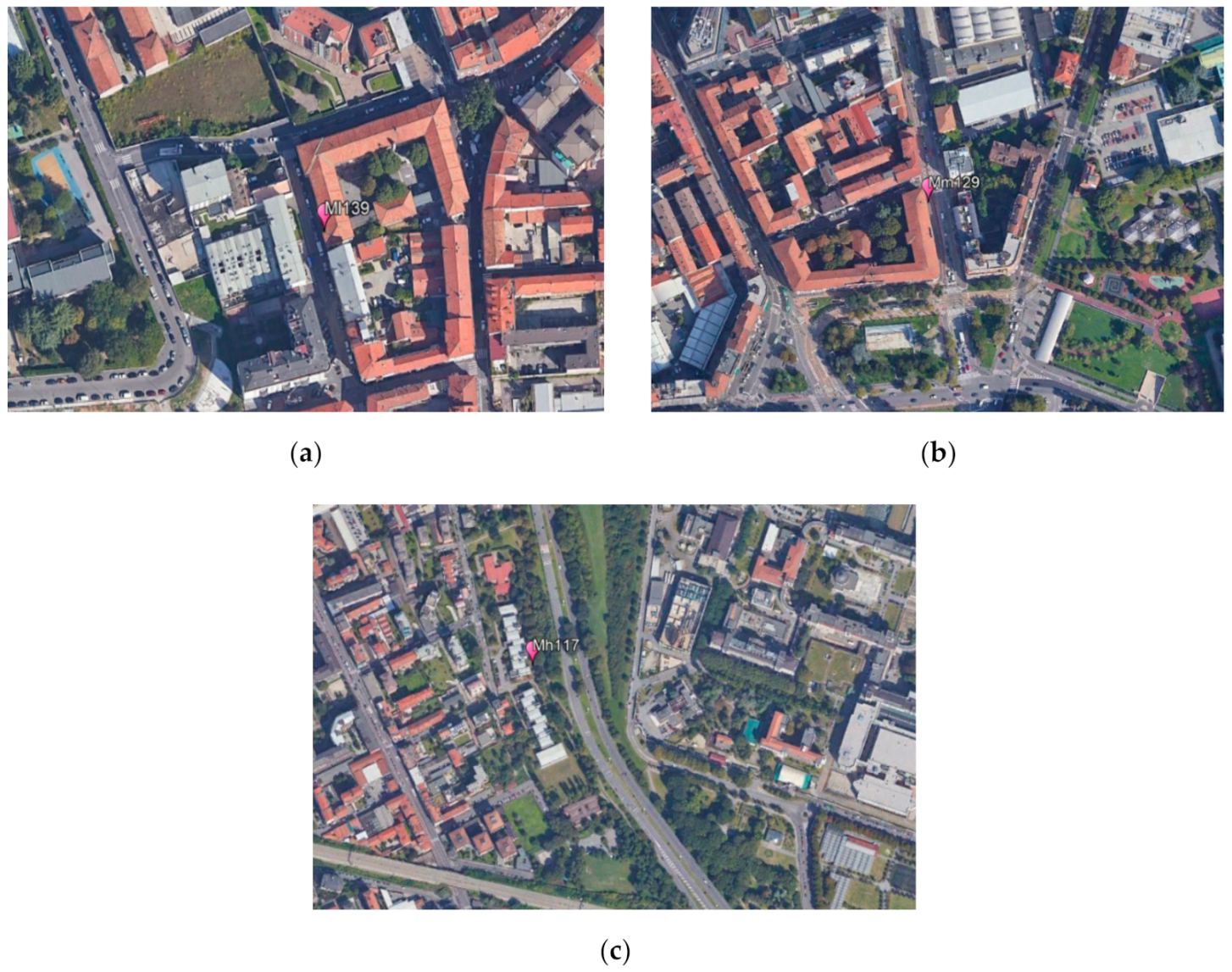
At each site, the environmental noise was monitored by an operator on two days (Wednesday, 21 March 2018 and Sunday, 15 April 2018), in order to obtain data on a weekday and during weekend, considering that specially traffic presents different intensities, depending on traffic to school and work or leisure. At all the three sites, the source recognition provided by the ANED procedure, since it was in its preliminary application, was manually validated by an expert.

2.1.2. Milan, Italy

Three sites were selected from the permanent continuous noise monitoring network operating in the northern part of the city, in a strongly built-up area with high population density and a widespread road network [22]. They represent roads with low, medium, and high traffic flow (Figure 2). In particular, site Ml139 (Figure 2a) is a local road surrounded by a school and residential buildings with low (l) traffic flow (<1000 vehicles in 24 h); site Mm129 (Figure 2b) is also a local road surrounded by a school, residential buildings, a chemical industry, and a park, but with a moderate (m) traffic flow (1000–10,000 vehicles in 24 h). Site Mh117 (Figure 2c) is near a thoroughfare road with high (h) capacity traffic flow (>10,000 vehicles in 24 h). At each site, the unattended monitoring data were collected at the same date (Tuesday, 26 March 2019).

2.2. Data Processing

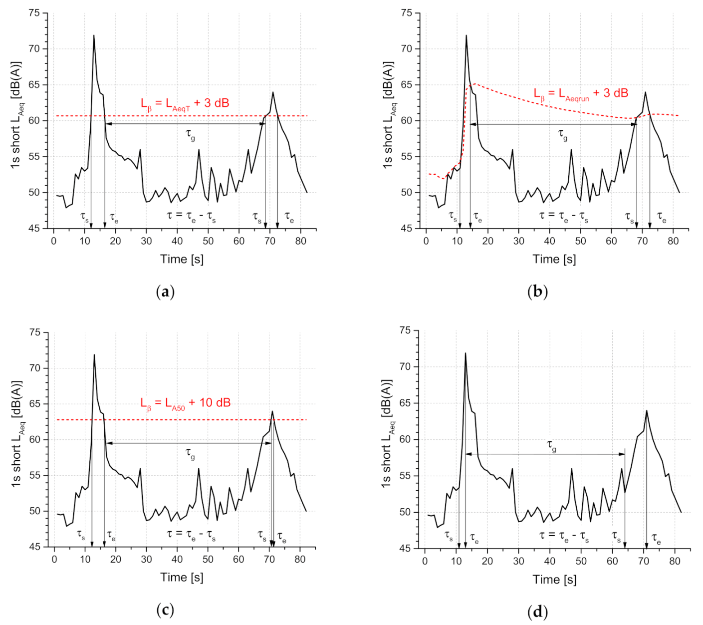
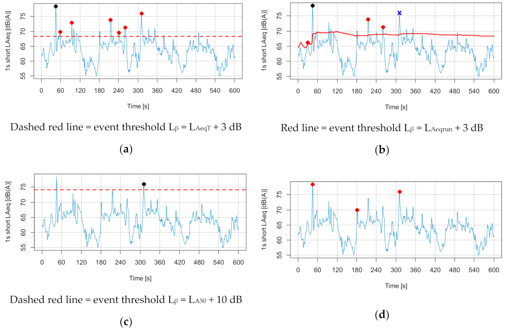
2.2.1. Detection of Noise Events

Individual events in the sound pressure level (SPL) time history of the environmental noise are usually identified by an exceedance-based detection algorithm. As detailed in the extensive literature review reported in [15], the onset of a noise event is detected when the instantaneous SPL exceeds a threshold level L_β for a duration τ in s, and with an emergence of at least E dB. Noise events are only retained when the time gap (or noise free interval) since the previous detected event is larger than τ_g [16].

A script running in the “R” environment, version 3.6.3 [25], was developed to import each of the 1 s short L_Aeq time series as input in a text file format, formed by four columns; that is date, time, short L_Aeq,1s in dB(A) at 1 s interval, and a label indicating the corresponding source, namely road traffic noise (RTN) or something else (ANE; anomalous noise event), as recognized by the ANED procedure [19].

Among the several criteria proposed to detect noise events, the following were considered (Figure 3), consider the outcome of the extensive studies carried out in [15,16]:

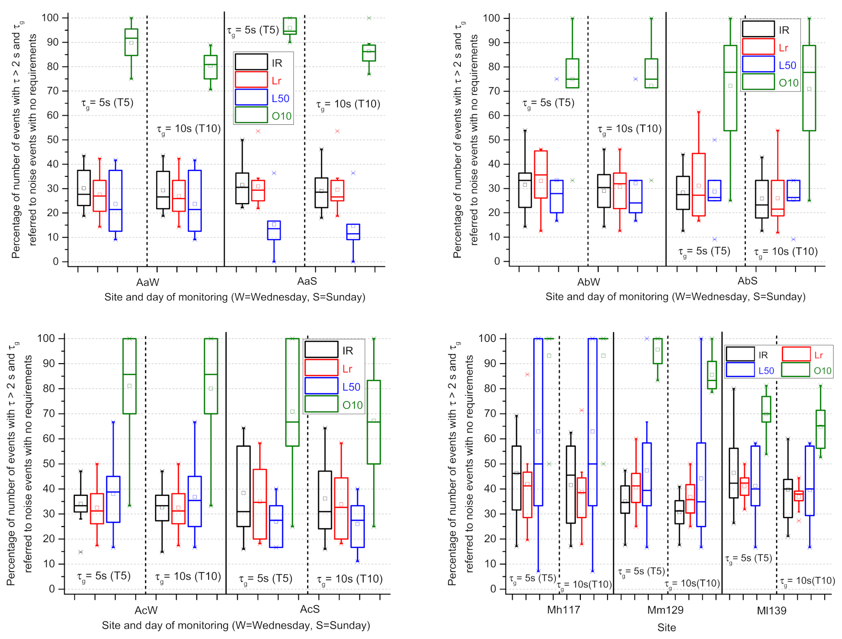
• Noise levels exceeding the threshold Lβ = LAeqT + C dB, according to the formulation of the intermittency ratio (IR) [17], where LAeqT is the continuous equivalent level referred to the measurement time T and 3 dB is the value chosen for the constant term C [17] (Figure 3a). This algorithm is denoted as “IR” hereinafter.
• Noise levels exceeding the threshold Lβ = LAeq,run + 3 dB, where LAeq,run is the running LAeq (Figure 3b). This algorithm is denoted as “Lr” hereinafter.
• Noise levels exceeding the threshold Lβ = LA50 + 10 dB, namely the NAL50E10 metric [16], where LA50 is the 50th noise level percentile; that is the noise level exceeded for 50% of the measurement time T (Figure 3c). This algorithm is denoted as “L50” hereinafter.
• SPL onset, as sum of progressive positive SPL increments, greater than 10 dB from the event start time τs (Figure 3d). This algorithm is denoted as “O10” hereinafter.

Each of the above algorithms were applied to detect noise events in the 1 s short L_Aeq,1s time series with the following options:

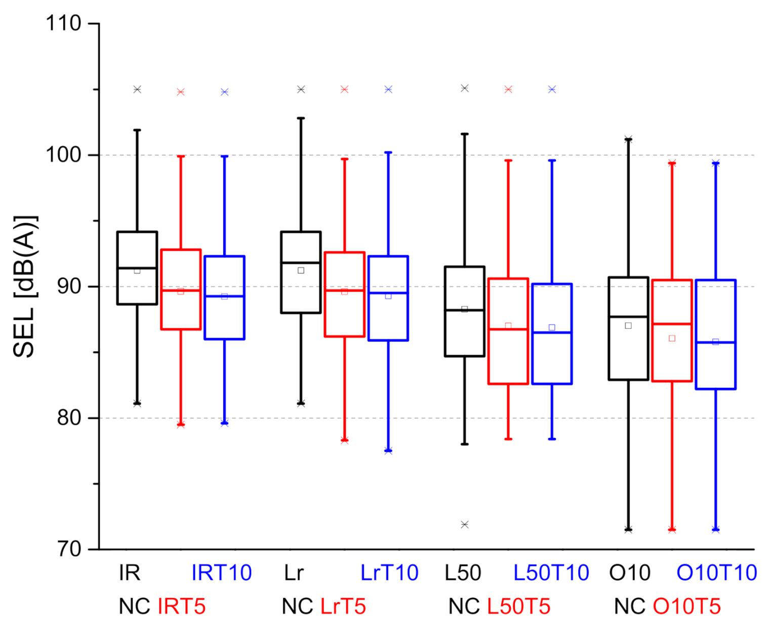
• Without any condition on the event duration τ and time gap τ_g (or noise free interval) between adjacent events, hereinafter denoted as NC.
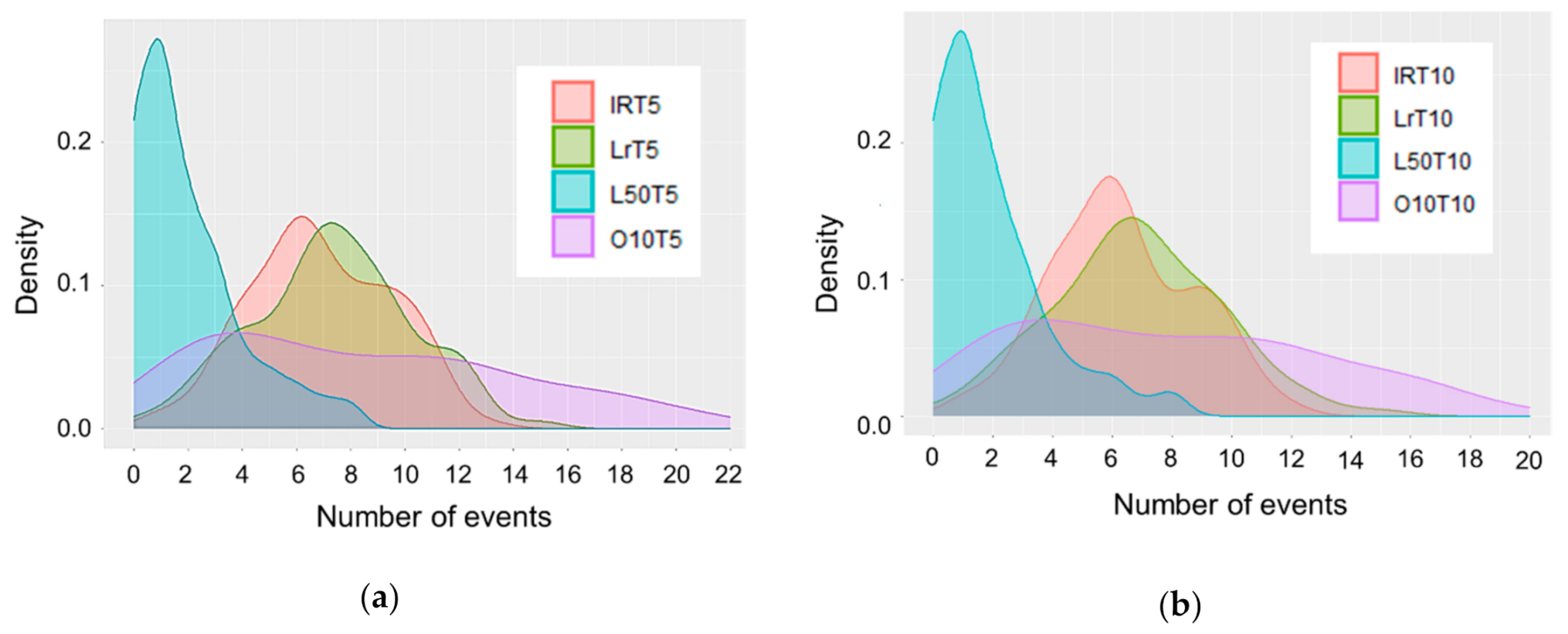
• Event duration τ > 2 s and time gap τ_g equal to 5 (T5) and 10 (T10) s, hereinafter denoted as C.

When a sound event was detected, in order to assign the relevant source, the labels provided by the ANED procedure at each second along the duration of the sound event itself were considered. The source was assigned according the following rules:

• Unique source labels, assigned source corresponding to that indicated by all the labels when they were always the same (either road traffic noise (RTN), or something else, i.e., anomalous noise event (ANE).
• Mixed source labels, assigned source corresponding to that indicated by the majority of the labels when they differed.
• Equal number of RTN and ANE labels, no source assignment.

In the algorithm Lr the term of +3 dB added to the running L_Aeq,run was chosen because this quantity roughly corresponds to a perception of a clear difference in SPL. The algorithms L50 and O10 seem suitable for detection of “notice-events”; that is, those potentially attracting attention and likely causing reactions by exposed people, for instance in terms of annoyance and sleep interference [23,26]. The algorithm O10 differs from the others because it only considers progressive positive SPL increments and not the decreasing SPL transients. The onset of 10 dB is often used as exceedance threshold to detect sound events, such as in the NAL50E10 index [16] and in the Italian legislation on railway and aircraft noise [27]. We should note that a difference of 10 dB in SPL roughly corresponds to a doubling of loudness.

The output of the data processing included the following outcomes:

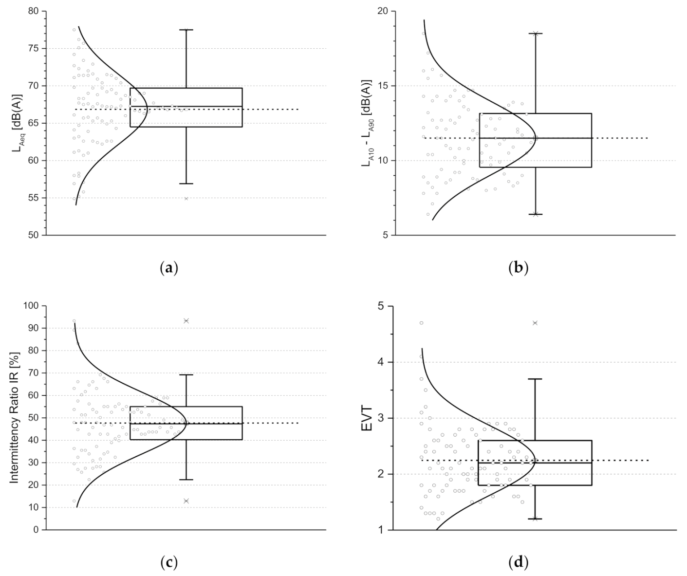
• The continuous equivalent level L_Aeq,T in dB(A), referred to measurement time T of 10 min.
• The running equivalent level L_Aeq,run in dB(A).
• The standard deviation (sdL_A) and the kurtosis (kL_A) of the 1 s short L_Aeq levels during the measurement time T to describe the level distribution.
• The noise climate, as difference between the percentiles levels L_A10 and L_A90 in dB(A) along the measurement time T.
• The intermittency ratio (IR) in %, calculated according to [17].
• The event-related component EVT of the Harmonica index [24], representing the acoustic energy provided by noise peaks that emerged above the background noise, and calculated as follows:

$$EVT=0.25·\left(L_{Aeq,T}-L_{A95eq}\right),$$

(1)

where L_A95eq is the equivalent background noise level, evaluated every second by the noise level exceeded 95% of the time during the previous T/6 interval, where T is the measurement time. We should note that the Harmonica index was formulated to provide information that is easier to understand by people and more closely reflects the noise nuisances, as perceived by the public.

• The total number of noise events detected by the four algorithms with (C) and without (NC) conditions on event duration and time gap.
• Start time τ_s, duration τ, SEL and L_Aeq levels of each detected noise event.
• Number of detected noise events.
• Number of noise events due to mixed sources as recognized by the ANED procedure [19].
• Number of noise events due to road traffic noise recognized as unique labels or majority of mixed labels as provided by the ANED procedure [19].
• Number of noise events with an equal number of RTN and ANE labels.
• Plot of 1 s short L_Aeq levels versus time, with indication of the detected noise events and the recognized source for each algorithm.

An example of the plots obtained from the data processing is given in Figure 4, regarding the noise monitoring at site Mh117 taken at 9:10 a.m., with a standard deviation sdL_A of L_Aeq,1s equal to 3.8 dB(A), and kurtosis kL_A = 3.1, close to the value of 3 corresponding to the normal distribution of SPLs. As shown in Figure 4, the detected noise events depend on the applied algorithms, as they can be different in number, detected at different times, can have different durations, and a set of source labels that lead to different source associations; moreover, all of the methods focus on different characteristics and features from the types of noise. For instance, setting the time gap between events τ_g = 5 s and the event duration τ > 2 s, algorithm IR detects 7 noise events (6 RTN + 1 ANE), algorithm Lr detects 5 noise events (3 RTN + 1 ANE + 1 not associated source), algorithm L50 detects 1 ANE event, and algorithm O10 detects 3 RTN events. Thus, it is clear that the choice of the noise event detection algorithm is important.

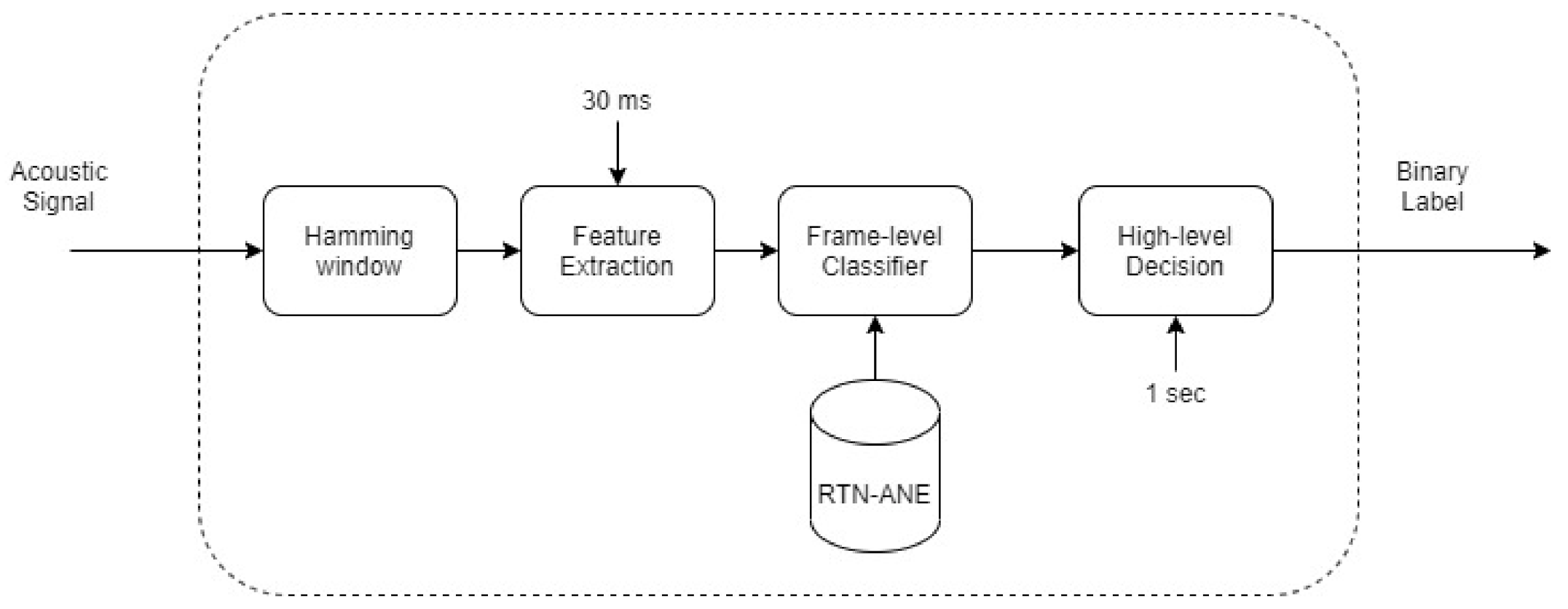
2.2.2. Recognition of the Noise Event Source

The ANED algorithm, designed in the framework of the DYNAMAP (dynamic noise mapping) project [28], is a two-stage decision scheme, as shown in Figure 5. At the first level, ANED classifies the acoustic signal at a frame-level base. It is based on a two-class detection-by-classification [29] approach, using an artificial intelligence algorithm trained by means of acoustic models from representative real-life data collected from both suburban and urban environments. In order to generate the frame-level label every 30 ms, the acoustic signal is analyzed by means of a feature extraction stage. This short-term windowing of the acoustic signal is performed by means of a Hamming window of 30 ms, with an overlap between windows of 50% of the signal, followed by a feature extraction step based on the Mel-frequency cepstral coefficient (MFCC) [30]. This feature extraction is followed by a Gaussian mixture model (GMM)-based binary classification stage [28]. The second level, a high-level decision, based on a majority vote criterion, had to be conducted every second, and it considered the aggregated values of the frame-level decisions, in a predefined time window, to generate a binary output (RTN/ANE). Both levels require a real-time implementation in-situ in the sensor gathering the data in order to provide the final binary label at the moment of the L_Aeq evaluation. The ANED algorithm was trained using more than 150 h of expert-manually labeled data, coming from the 24 sensors, deployed by the DYNAMAP project in Milan, with around 8% of anomalous noise events (e.g., bird singing, sirens, dogs barking, horns, trams). The diversity coming from 24 sensors—some from narrow streets, others in wide ones, some close to parks, and others close to schools—gave the dataset a variate group of examples of urban sounds. The ANED procedure was already tested and validated in a real environment in the framework of the LIFE DYNAMAP project [28,31,32]. A further study [29] showed an accuracy of more than 70% in urban environment ANE detection, measured at frame level (using a 30-ms window analysis), by means of a 10-fold cross-validation test to ensure the stability of the results. The performance of the ANED algorithm was also validated in other environments [18], considering, in addition, the acoustic salience of the ANEs in real-operation [33]. The validation was inspired on the manual evaluation process by experts, considering the most salient events present in the measurements, with respect to the L_Aeq1s. The algorithm detected—for the events catalogued as high-salience—all of the present airplane noise, more than 90% of works, and people talking, and for the mid-high salience, more than 84% of airplane noise, nearly 80% of works, and more than 60% of people talking, to list a few examples. The accuracy results of the ANED algorithm is especially improved with a high-level stage, and it shows good performance, especially when dealing with high salience events.

3. Results and Discussion

Figure 6 reports the box plots of the acoustic parameters L_Aeq, the noise climate L_A10–L_A90, the intermittency ratio (IR), and the event component (EVT) of the Harmonica index for all 92-time series, together with the estimated normal distribution curve on the left side of each box plot. The variability is fairly large and covers a reasonable range of environmental noise time patterns, usually occurring in urban areas. The available data did not include the spectrum and the overall unweighted dB level and, therefore, the analysis was limited to dB(A) data. However, these types of data are, very often, the output of the noise monitoring networks usually installed in urban areas, mainly to check the compliance of the environmental noise with the limits issued by the legislation.

Since, at least at the Milan sites, it was not possible to check whether the noise events detected by the four algorithms matched with their real occurrences during the monitoring time, the analysis was aimed to compare the considered detection algorithms. The number of events detected by each of the four algorithms is reported in the box plots of Figure 7, for every site and day of monitoring.

Algorithms IR and Lr provided rather similar results, the number of events detected by the former (1889 events) being −6% on average less than those (2010) detected by the latter. A large difference was observed in the number of noise events detected by the above two algorithms and those recognized by the algorithms L50 (685, the lowest number of events) and O10 (929). These two algorithms on average detected −59% of events than those recognized by IR and Lr. The algorithms IR and Lr in their definition differed for the threshold, with the former having a fixed value equal to L_AeqT, referred to the measurement time (T), and the latter an adaptive value equal to the running L_Aeq,run, while for both, the exceedance (E) above the threshold was equal to 3 dB. In particular, IR detected a higher number of events than that obtained for Lr for 42% of the 92-time histories of 1 s A-weighted short L_Aeq, a lower one for 50%, and the same number for 8%. As mentioned above, the algorithms L50 and O10 seem suitable to detect notice-events; the former having a fixed threshold equal to L_A50 + 10 dB and the latter looking at a sum of progressive increases of the A-weighted SPL greater than 10 dB from the SPL at the event start time τ_e (see Figure 3). We should note that, in Milan, the site with high traffic flow (MhT) showed a number of events lower than those observed for moderate (MmT) and low (MlT) traffic flow for all algorithms. This was most likely due to the louder background noise produced by the higher number of vehicles passing-by, as confirmed by the intermittency ratio equal to 31.3%, on average, for MhT, compared to 44.3% and 63.4% for MmT and MlT, respectively.

Figure 8 reports the box plots of the percentage of the number of events with conditions (C), referred to those without conditions (NC) and detected by the four algorithms, at each site and day of monitoring in compliance with an event duration τ longer than 2 s, and a time gap between events τ_g of 5 (T5) or 10 s (T10).

The considered conditions for the noise events largely reduce the number of detected noise events compared to those without conditions (NC), with the exception of the O10 algorithm. This suggests that most noise fluctuations are not recognized as noise events.

Regarding noise exposure, Figure 9 shows the box plots of SEL values for not conditioned (NC) events versus conditioned events detected by the four algorithms. The SEL values for conditioned events are generally lower than those for not conditioned (NC) ones, as reported in

Table 1. Differences of SEL values for conditioned (C) minus not conditioned (NC) events detected by the four algorithms; p values reported in bold correspond to not significant differences at 95% confidence level.

	IRT5	IRT10	LrT5	LrT10	L50T5	L50T10	O10T5	O10T10
Median	−1.2	−1.6	−1.3	−1.6	−1.5	−1.4	−0.4	−0.9
MAD	0.4	0.7	0.6	0.8	1.4	1.4	0.4	0.9
pvalue
Not conditioned events (NC) vs. Conditioned (C)	0.016	0.037	0.020	0.006	0.115	0.083	0.331	0.186
T5 vs. T10	0.528		0.646		0.894		0.705

, where median and median absolute deviation (MAD) values are given for the SEL differences conditioned—not conditioned (NC) events across all data. The largest values of MAD (1.4) are observed for the L50 algorithm. Table 1 also gives the p-values obtained by the Wilcoxon test, a non-parametric statistical test to compare two paired groups, reported in bold when there were non-significant differences at the 95% confidence level observed. These non-significant differences were obtained for the L50 and O10 algorithms, as well as for all the algorithms when comparing the SEL values obtained with a time gap τ_g of 5 (T5) and 10 (T10) s.

Considering the labels provided by the ANED procedure at each second of every single event, and the rules to assign the relevant source described in Section 2.2.1,

Table 2. Percentage of events detected by the four algorithms for the two time gaps between events of 5 (T5) and 10 s (T10) as function of the source type.

%	IRT5	LrT5	L50T5	O10T5	IRT10	LrT10	L50T10	O10T10
RTN	78.9	79.2	75.7	86.0	79.6	79.2	74.9	86.2
ANE	17.9	17.5	19.9	11.8	17.4	17.7	20.5	11.7
Mixed	33.0	34.0	40.3	30.3	32.5	33.4	39.8	31.0
Even	3.1	3.1	3.9	2.3	3.1	3.0	4.1	2.2

reports the percentage of events associated with road traffic noise (RTN), those with sources different from RTN (ANE), mixed events where labels RTN and ANE were present, and the source was assigned, according to the majority of labels of the same type (RTN or ANE), and sources not assigned because of the equal number of labels RTN and ANE in the event (reported as even).

Road traffic noise (RTN) is largely the source producing the events; the percentage of events for which the source is not assigned (even events) is limited to a small value (2–4%). Events that, during their duration, showed both RTN and ANE labels, was about 1/3 of the total.

The probability density plots of the number of events detected by each algorithm for both time gaps in each SPL time history, reported in Figure 10, show similar shapes for the time gaps. The sharper distribution and the lowest number of detected events is observed for the algorithm L50, whereas O10 shows the flattest shape.

Regarding the duration of the detected events, set to a minimum of 3 s, Figure 11 reports the box plot of the observed durations at each site detected by the IRT5 algorithm. The highest median values (5 s) were observed for the sites Ac on Sunday and Ab on Wednesday in Andorra, and site Ml139 in Milan. In all of these sites—road traffic was not the predominant noise source.

To get more insight on the relationships among the variables, further analysis was conducted to determine the patterns in the results obtained for the time series; that is the matrix formed by 92 observations and 15 variables, namely the acoustic metrics (L_Aeq, L_A10 − L_A90, IR, EVT), the descriptors of the SPL distribution (sL_A and kL_A), and the number of events detected by the four algorithms for the two time gaps between events. For this purpose, the principal component analysis (PCA) was performed using the FactoMineR package [34], considering the Euclidean distance between scaled observations (mean = 0, standard deviation = 1). The obtained variable correlation plot is given in Figure 12, where the variable’s contribution at the two dimensions is reported on a colored scale. The first two dimensions together explain a large percentage (70.15%) of the dataset variability. The L_Aeq level is the variable with the lowest contribution, confirming that this metric is not suitable to describe the presence of events.

The two time gaps between events led to similar results for each event detection algorithm; good correlation is observed between the intermittency ratio (IR) and the event component (EVT) of the Harmonica index, as shown in Figure 13. It is also confirmed that the algorithms L50 and O10, most likely suitable to detect notice-events, are correlated, and differ from the algorithms based on IR and Lr (see dimension 2).

Considering the features of the Harmonica index, which accounts for the noise energy content (by the background component, BGN), its eventfulness (by the event component, EVT), and its ease to be understood by people, we investigated its correlation with the SEL of events detected by the four algorithms. The results, in terms of linear regression, are shown in Figure 14, where the yellow and red bands on the x axis report the qualitative scale proposed for the Harmonica values [24]. All 92 SPL time histories are within the “noisy” and “very noisy” attributes of the scale. The regression is better for IR and Lr algorithms, very close to each other, than for L50 and O10. The threshold value of 8 for the Harmonica index, separating the “noisy” environment from the “very noise” environment, corresponds to different values for SEL, as shown in Figure 15. In particular, for procedures L50 and O10, suitable to detect “notice-events”, the SEL values corresponding to the threshold value of Harmonica are lower than those observed for the IR and Lr algorithms, most likely due to the temporal patterns of such notice-events (e.g., high SPL rise time). The variability range of each reported value was obtained, considering the prediction bands at the 95% confidence level.

4. Conclusions

The evaluation of human reactions to road traffic noise exposure might be improved by accounting for the occurrence of noise events in addition to the use of indicators based on sound energy. A wide range of procedures to detect such noise events were proposed in the literature, but there is yet no generally accepted algorithms. Considering the outcomes of the literature on this important topic, it was deemed of interest to examine four algorithms for noise event detection, as described in Figure 3—IR, Lr, L50, and O10. To evaluate the performance of these algorithms, they were applied to the sound monitoring data taken at six sites in urban areas, formed by 92 L_Aeq1s time histories. Three options were considered for the event detection—no condition on event duration τ and time gap between adjacent events τ_g, event duration τ > 2 s with time gap τ_g = 5 s, event duration τ > 2 s and time gap τ_g = 10 s. Moreover, the available data are able to label each 1 s short L_Aeq, accor ding to the binary classification obtained by the anomalous noise event detection (ANED) procedure, and discriminate road traffic noise (RTN) from other sources (ANE). This is a very important feature that improves the efficiency of noise mitigation actions, focusing on specific sources.

The results showed that the algorithms L50 and O10, owing to their definitions, seem more suitable to detect “notice-events”, e.g., events that, for their features, are clearly perceived and potentially affect the people who are exposed to them. These algorithms detect much less events than those recognized by the other two algorithms, namely IR and Lr. For all of the algorithms, the site in Milan with high traffic flow showed a number of detected events lower than those observed for moderate (MmT) and low (MlT) traffic flow, most likely due to the louder background noise produced by the higher number of vehicles passing-by. The conditions required for the events largely reduced the number of those recognized, with the exception of the O10 algorithm. In terms of noise exposure, the SEL values for the conditioned events were lower than those observed for not conditioned events. The ANED procedure showed that road traffic noise was largely the source producing the events (more than 70% of detected events for all algorithms). The principal component analysis showed that the two time gaps between events led to similar results for each event detection algorithm; moreover, good correlation was observed between the intermittency ratio (IR) and the event component (EVT) of the Harmonica index. Regarding this index, its linear regression with the SEL of events detected by the four algorithms provides interesting results. In particular, the value of 8 for the Harmonica index, separating the “noisy” from the “very noise” environments on the qualitative scale, corresponds to SEL values of about 92 dB and 88–89 dB for the IR and Lr couple and the L50 and O10 couple, respectively. This difference is most likely due to the different selections of events performed by the algorithms, with L50 and O10 more suitable for notice-events, characterized by specific temporal patterns (e.g., high SPL rise time).

The results cannot be generalized and are limited to the four algorithms considered. However, it seems that the L50 algorithm, providing the lowest number of events, is the least sensitive in detection; the performance of the O10 algorithm is less influenced by conditions required for noise events than observed for the other three algorithms. Beyond that, it is important to address the need for automatic procedures to detect noise events, include such events in sound environment descriptions, consider their harmful health effects and improve mitigation actions.

References

1. European Environment Agency. Good Practice Guide on Noise Exposure and Potential Health Effects; EEA Technical Report 11/2010; EEA: Copenhagen, Denmark, 2010. [Google Scholar]
2. Stansfeld, S.A.; Matheson, M.P. Noise pollution: Non-auditory effects on health. Br. Med. Bull. 2003, 68, 243–257. [Google Scholar] [CrossRef] [PubMed]
3. Fritschi, L.; Brown, A.L.; Kim, R.; Schwela, D.H.; Kephalopoulos, S. Burden of Disease from Environmental Noise. Quantification of Healthy Life Years Lost in Europe; World Health Organization Regional Office for Europe, JRC European Commission: Copenhagen, Denmark, 2011. [Google Scholar]
4. Directive 2002/49/EC of the European Parliament and of the Council of 25 June 2002 relating to the assessment and management of environmental noise. Off. J. Eur. Communities 2002, 189, 12.
5. Kephalopoulos, S.; Paviotti, M.; Anfosso-Lédée, F. Common Noise Assessment Methods in Europe (CNOSSOS-EU); Publications Office of the European Union: Luxembourg, 2012. [Google Scholar]
6. Bertrand, A. Applications and trends in wireless acoustic sensor networks: A signal processing perspective. In Proceedings of the 18th IEEE Symposium on Communications and Vehicular Technology in the Benelux (SCVT), Ghent, Belgium, 22–23 November 2011; pp. 1–6. [Google Scholar]
7. Alsina Pagès, R.M.; Alias, F.; Bellucci, P.; Cartolano, P.; Coppa, I.; Peruzzi, L.; Bisceglie, A.; Zambon, G. Noise at the time of COVID 19: The impact in some areas in Rome and Milan, Italy. Noise Mapp. 2020, 7, 248–264. [Google Scholar] [CrossRef]
8. Bockstael, A.; De Coensel, B.; Lercher, P.; Botteldooren, D. Influence of temporal structure of the sonic environment on annoyance. In Proceedings of the 10th International Congress on Noise as a Public Health Problem (ICBEN), London, UK, 24–28 July 2011; pp. 945–952. [Google Scholar]
9. De Coensel, B.; Botteldooren, D.; De Muer, T.; Berglund, B.; Nilsson, M.E.; Lercher, P. A model for the perception of environmental sound based on notice-events. J. Acoust. Soc. Am. 2009, 126, 656–665. [Google Scholar] [CrossRef] [PubMed]
10. Lercher, P. Environmental noise and Analysis of an Annotated health: An integrated research perspective. Environ. Int. 1996, 22, 117–129. [Google Scholar] [CrossRef]
11. Vidaña-Vila, E.; Duboc, L.; Alsina-Pagès, R.M.; Polls, F.; Vargas, H. BCNDataset: Description and night urban leisure sound dataset. Sustainability 2020, 12, 8140. [Google Scholar] [CrossRef]
12. Brambilla, G.; Confalonieri, C.; Benocci, R. Application of the intermittency ratio metric for the classification of urban sites based on road traffic noise events. Sensors 2019, 19, 5136. [Google Scholar] [CrossRef] [PubMed] [Green Version]
13. Brambilla, G.; Benocci, R.; Confalonieri, C.; Roman, H.E.; Zambon, G. Classification of urban road traffic noise based on sound energy and eventfulness indicators. Appl. Sci. 2020, 10, 2451. [Google Scholar] [CrossRef] [Green Version]
14. Brown, A.L.; Banerjee, D.; Tomerini, D. Noise events in road traffic and sleep disturbance studies. In Proceedings of the Internoise 2012, New York, NY, USA, 19–22 August 2012. [Google Scholar]
15. Brown, A.L.; De Coensel, B. A study of the performance of a generalized exceedance algorithm for detecting noise events caused by road traffic. Appl. Acoust. 2018, 138, 101–114. [Google Scholar] [CrossRef] [Green Version]
16. De Coensel, B.; Brown, A.L. Event-based Indicators for road traffic noise exposure assessment. In Proceedings of the Euronoise 2018, Crete, Greece, 27–31 May 2018; pp. 485–490. [Google Scholar]
17. Wunderli, J.M.; Pieren, R.; Habermacher, M.; Vienneau, D.; Cajochen, C.; Probst-Hensch, N.; Röösli, M.; Brink, M. Intermittency ratio: A metric reflecting short-term temporal variations of transportation noise exposure. J. Expo. Sci. Environ. Epidemiol. 2016, 26, 575–585. [Google Scholar] [CrossRef] [PubMed]
18. Orga, F.; Alías, F.; Alsina-Pagès, R.M. On the impact of anomalous noise events on road traffic noise mapping in urban and suburban environments. Int. J. Environ. Res. Public Health 2018, 15, 13. [Google Scholar] [CrossRef] [PubMed] [Green Version]
19. Socoró, J.C.; Ribera, G.; Sevillano, X.; Alías, F. Development of an anomalous noise event detection algorithm for dynamic road traffic noise mapping. In Proceedings of the ICSV 2015, Florence, Italy, 12–16 July 2015. [Google Scholar]
20. Bellucci, P.; Peruzzi, L.; Zambon, G. LIFE DYNAMAP: Making dynamic noise maps a reality. In Proceedings of the Euronoise 2018, Crete, Greece, 27–31 May 2018; pp. 1181–1188. [Google Scholar]
21. Alsina-Pagès, R.M.; Almazán, R.G.; Vilella, M.; Pons, M. Noise events monitoring for urban and mobility planning in Andorra la Vella and Escaldes-Engordany. Environments 2019, 6, 24. [Google Scholar] [CrossRef] [Green Version]
22. Benocci, R.; Confalonieri, C.; Roman, H.E.; Angelini, F.; Zambon, G. Accuracy of the dynamic acoustic map in a large city generated by fixed monitoring units. Sensors 2020, 20, 412. [Google Scholar] [CrossRef] [PubMed] [Green Version]
23. Brink, M.; Schäffer, B.; Vienneau, D.; Foraster, M.; Pieren, R.; Eze, I.C.; Cajochen, C.; Probst-Hensch, N.; Röösli, M.; Wunderli, J.-M. A survey on exposure-response relationships for road, rail, and aircraft noise annoyance: Differences between continuous and intermittent noise. Environ. Int. 2019, 125, 277–290. [Google Scholar] [CrossRef] [PubMed]
24. Mietlicki, C.; Mietlicki, F.; Ribeiro, C.; Gaudibert, P.; Vincent, B. The HARMONICA project, new tools to assess environmental noise and better inform the public. In Proceedings of the Forum Acusticum 2014, Kraków, Poland, 7–12 September 2014. [Google Scholar]
25. R Core Team. R: A Language and Environment for Statistical Computing; R Foundation for Statistical Computing: Vienna, Austria, 2018; Available online: https://www.R-project.org/ (accessed on 28 August 2021).
26. Lercher, P.; Boeckstael, A.; De Coensel, B.; Dekoninck, L.; Botteldooren, D. The application of a notice-event model to improve classical exposure-annoyance estimation. In Proceedings of the Acoustics 2012, Hong Kong, China, 13–18 May 2012. [Google Scholar]
27. Decree of the Italian Ministry of Environment, D.M. Ambiente 16/3/1998 Tecniche di rilevamento e di misurazione dell’inquinamento acustico (Measurement techniques of noise pollution). Gazz. Uff. 1998, 76, 15–19. (In Italian) [Google Scholar]
28. Sevillano, X.; Socoró, J.C.; Alías, F.; Bellucci, P.; Peruzzi, L.; Radaelli, S.; Coppi, P.; Nencini, L.; Cerniglia, A.; Bisceglie, A.; et al. DYNAMAP—Development of low cost sensors networks for real time noise mapping. Noise Mapp. 2016, 3, 172–189. [Google Scholar] [CrossRef]
29. Socoró, J.C.; Alías, F.; Alsina-Pagès, R.M. An anomalous noise events detector for dynamic road traffic noise mapping in real-life urban and suburban environments. Sensors 2017, 17, 2323. [Google Scholar] [CrossRef] [PubMed]
30. Mermelstein, P. Distance measures for speech recognition, psychological and instrumental. Pattern Recognit. Artif. Intell. 1976, 116, 374–388. [Google Scholar]
31. Alías, F.; Socoró, J.C.; Alsina-Pagès, R.M. WASN-based day–night characterization of urban anomalous noise events in narrow and wide streets. Sensors 2020, 20, 4760. [Google Scholar] [CrossRef] [PubMed]
32. Orga, F.; Socoró, J.C.; Alías, F.; Alsina-Pagès, R.M.; Zambon, G.; Benocci, R.; Bisceglie, A. Anomalous noise events considerations for the computation of road traffic noise levels: The DYNAMAP’s Milan case study. In Proceedings of the 24th International Congress on Sound and Vibration, ICSV 2017, London, UK, 23–27 July 2017. [Google Scholar]
33. Alsina-Pagès, R.M.; Alías, F.; Socoró, J.C.; Orga, F. Development and validation of an anomalous noise events detector focused on salient events through an urban and suburban WASN adapted to real-operation. In Proceedings of the ICSV27, online, 11–16 July 2021. [Google Scholar]
34. Lê, S.; Josse, J.; Husson, F. FactoMineR: An R Package for Multivariate Analysis. J. Stat. Softw. 2008, 25, 1–18. [Google Scholar] [CrossRef] [Green Version]
Figure 1. Sites in Andorra la Vella selected for noise monitoring (satellite images from Google Earth Pro 7.3.4.8248) [21]: (a) Site “Aa” Ctra. de l’Obac/Carrer de la Unió; (b) Site “Ab” Av. Carlemany/Carrer de la Valira; (c) Site “Ac” Av. Meritxell no. 73.
Applsci 11 08031 g001
Figure 2. Sites in Milan selected for noise monitoring (satellite images from Google Earth Pro 7.3.4.8248) [22]: (a) Site “Ml139” Via Leonardo Bruni; (b) Site “Mm129” Via Benigno Crespi; (c) Site “Mh117” Viale Enrico Fermi.
Applsci 11 08031 g002
Figure 3. Parameters of the sound event detection for each algorithm: (a) algorithm “IR” based on IR; (b) algorithm “Lr” based on LAeq,run; (c) algorithm “L50” based on LA50; (d) algorithm “O10” based on the sum of progressive increments of SPL. τ is the duration of the sound event, starting at time τs and ending at time τe, and τg is the time gap between sound events.
Applsci 11 08031 g003
Figure 4. Example of plots obtained from the data processing setting time gap between events τg = 5 s and event duration τ > 2 s. Red and black dots mark events due to road traffic and other sources, respectively; blue cross mark event with not assigned source: (a) algorithm “IR”; (b) algorithm “Lr”; (c) algorithm “L50”; (d) algorithm “O10”.
Applsci 11 08031 g004
Figure 5. ANED computation block diagram, with a first filtering stage, a feature extraction algorithm (MFCC) every 30-msec window, and a frame-level classifier, with a final high-level decision based on a majority vote every 1 s.
Applsci 11 08031 g005
Figure 6. Box plots of the acoustic parameters observed for all 92-time series: (a) the equivalent level LAeq; (b) the noise climate LA10–LA90; (c) the intermittency ratio (IR); (d) the event component (EVT) of the Harmonica index.
Applsci 11 08031 g006
Figure 7. Box plots of the number of noise events detected by each algorithm for every site and day of monitoring (W = Wednesday, S = Sunday, T = Tuesday).
Applsci 11 08031 g007
Figure 8. Box plots of the percentage of the number of conditioned events, referred to those “not conditioned”, and detected by the four algorithms, at each site and day of monitoring, in compliance with an event duration > 2 s and a time gap between events τg of 5 (T5) or 10 s (T10).
Applsci 11 08031 g008
Figure 9. Comparison of box plots of SEL for not conditioned (NC) events versus conditioned events detected by the four algorithms.
Applsci 11 08031 g009
Figure 10. Density plots of the number of events detected in each SPL time history by the four algorithms for the two time gaps between events: (a) τg = 5 s (T5); (b) τg = 10 s (T10).
Applsci 11 08031 g010
Figure 11. Box plots of the event durations at each site detected by the IRT5 algorithm: (a) Andorra’s sites; (b) Milan’s sites.
Applsci 11 08031 g011
Figure 12. Correlation plot obtained by the PCA and variable contribution on a colored scale.
Applsci 11 08031 g012
Figure 13. Regression plot between intermittency ratio (IR) and the event component (EVT) of the Harmonica index; confidence and prediction bands at 95% confidence level.
Applsci 11 08031 g013
Figure 14. Regression plots between the Harmonica index and the SEL values of the events detected by the four algorithms: (a) IR algorithm; (b) L50 algorithm; (c) Lr algorithm; (d) O10 algorithm; confidence and prediction bands at the 95% confidence level.
Applsci 11 08031 g014
Figure 15. Linear regression fitting between the Harmonica index and the SEL values of events detected by the four algorithms; SEL values corresponding to Harmonica index = 8 are reported, with their variability range obtained by the prediction bands at the 95% confidence level.
Applsci 11 08031 g015