Abstract
Reliable estimates of peak particle velocity (PPV) from blasting-induced vibrations at a construction site play a crucial role in minimizing damage to nearby structures and maximizing blasting efficiency. However, reliably estimating PPV can be challenging due to complex connections between PPV and influential factors such as ground conditions. While many efforts have been made to estimate PPV reliably, discrepancies remain between measured and predicted PPVs. Here, we analyzed various methods for assessing PPV with several key relevant factors and 1191 monitored field blasting records at 50 different open-pit sites across South Korea to minimize the discrepancies. Eight prediction models are used based on artificial neural network, conventional empirical formulas, and multivariable regression analyses. Seven influential factors were selected to develop the prediction models, including three newly included and four already formulated in empirical formulas. The three newly included factors were identified to have a significant influence on PPV, as well as the four existing factors, through a sensitivity analysis. The measured and predicted PPVs were compared to evaluate the performances of prediction models. The assessment of PPVs by an artificial neural network yielded the lowest errors, and site factors, K and m were proposed for preliminary open-pit blasting designs.
1. Introduction
Drilling and blasting is typically used to fragment rock masses at various building and civil construction sites because it is the most economical means of breaking rock for excavation. However, blasting at construction sites is accompanied by undesirable environmental side effects, such as vibration, noise, and scattering of debris. According to Korea’s Office of National Environmental Conflict Resolution Commission, 3840 (approximately 84%) of the 4557 environmental dispute cases on record involve noise and vibration, primarily from construction sites [1]. Blasting vibrations occurring at a construction site account for the majority of these environmental disputes because they result in damage to nearby structures and present various safety concerns. Every country specifies a limit on the peak particle velocity (PPV) of the induced vibrations to minimize damage to nearby structures. According to DIN 4150-3 [2], the limits on PPV are 2 cm/s for buildings used for commercial purposes, 0.5 cm/s for dwellings, and 0.3 cm/s for buildings under preservation orders at a frequency of 1 to 10 Hz. Siskind et al. [3] proposed that 1.9 and 1.3 cm/s are safe levels of blasting vibration for drywall and plaster under 10 Hz conditions. In South Korea, the limits on PPV are 0.2 cm/s for cultural assets and 0.5 cm/s for apartments. Blasting engineers try to accurately predict PPVs that will be induced by blasting and apply the predicted PPVs to the design of blasting patterns to comply with these regulations. Many researchers have studied and proposed various empirical formulas to predict and control PPV [4]. Among the various empirical formulas, a conventional empirical formula developed by U.S. Bureau of Mines (USBM) researchers, Duvall and Petkof [5] has been widely used to predict PPV and design blasting patterns. The current design approach consists of two steps. First, several test blastings are conducted to determine site factors K and m, which represent geological characteristics, before massive blasting. At each test, the distances between blasting and monitoring points, the charge weights per delay, and the PPVs are monitored and recorded. Based on these factors, K and m are calculated. Second, PPV is predicted using an empirical formula with K, m, the distance between blasting and monitoring points, and the charge weight per delay. However, this empirical formula often results in significant discrepancies between measured and predicted PPVs. Due to the discrepancies, blasting engineers are forced to use a high factor of safety (FoS) to prevent problems resulting from excessive vibration velocity. A high FoS typically requires the use of a more conservative charge weight per delay than the maximum allowable weight would accommodate. The conservative charge weight per delay can decrease blasting efficiency and increase construction time and total cost. A more accurate method of predicting PPV is vital to protect the environment and increase the efficiency of blasting.
The artificial neural network (ANN) has been applied in various fields such as renewable energy systems [6], atmospheric science [7], and civil engineering [8,9] to predict targets. In addition, research is also ongoing on predicting PPVs using ANN. To develop an ANN model for PPV prediction, Nguyen et al. [10] gathered 185 blasting datasets from a limestone mine in Vietnam, Azimi et al. [11] collected 70 blasting datasets from a copper mine in Iran, and Bui et al. [12] obtained 83 blasting datasets from a quarry mine in Vietnam. Every result of the research showed good agreement with the measured and predicted PPVs. ANN is generally not limited by any assumptions such as linearity or normality, thus ANN has the modeling power to derive excellent results even with irregular datasets and complex phenomena [13,14]. However, in the previous studies, the largest number of datasets was only 185 and the datasets were obtained from a limited local region. Each ANN model developed in the previous studies is only strictly applicable to the site where the study was conducted due to the limited region. Therefore, it is necessary to develop the global prediction model and to select influential factors which can be obtained easily from every blasting site. In this paper, an ANN was selected as one of the prediction methods due to its strengths. Its performance for predicting PPVs was compared with the performances of conventional empirical formulas and multivariate regression analyses to find the best prediction methods for predicting PPVs with numerous datasets of field blasting records from various sites.
2. Methodology
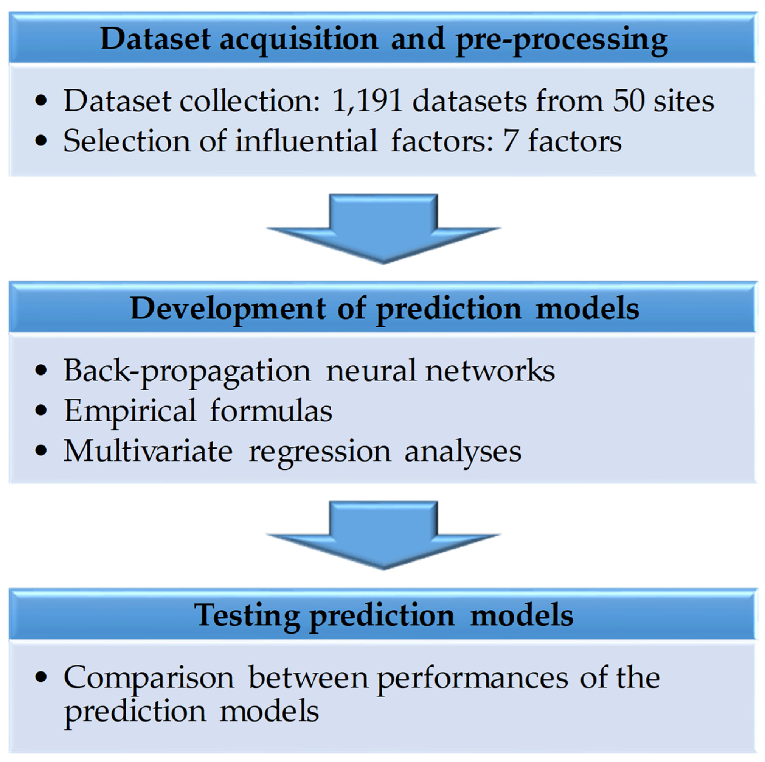
Figure 1 shows the process for this study, which consists of three steps; acquisition and pre-processing of blasting datasets, development of prediction models using three other methods, and testing and comparison of the prediction models.
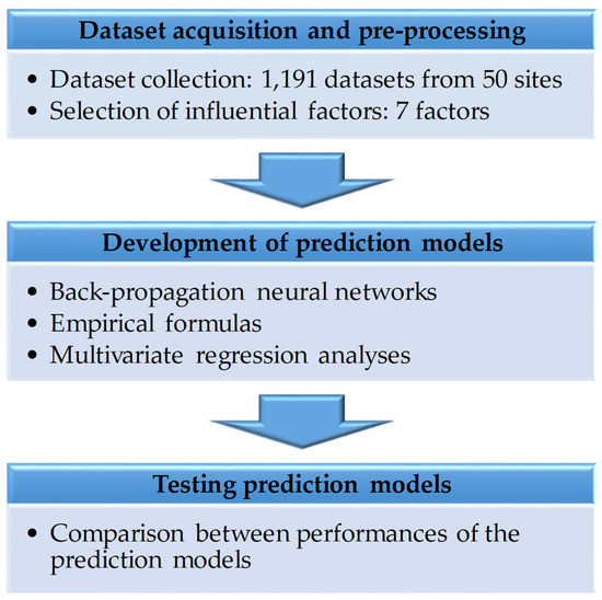
Figure 1.
Three steps of the research process.
2.1. Artificial Neural Network
An ANN is a prediction method based on causes and effects obtained through experience. It can be used as a tool for training, remembering, and analyzing using the computational power of a computer [15]. The network calculates non-linear and complex connections with an input layer, a hidden layer, and an output layer. Each layer has a node for calculation, and their weights and biases act as interlayer connections. The input and output layers consist of causal and result parameters, respectively. The training algorithm of the ANN used in this study was back-propagation, which is the most efficient ANN training algorithm available [16,17]. In back-propagation, the output values calculated in the forward direction through weights and biases are used to calculate training errors from the true values. Through these errors, weights and biases are corrected to minimize the errors in the reverse direction. These sequences repeat until the errors meet the convergence tolerance or other limit conditions. After the ANN model meets the conditions, it can be used as a prediction model with final weights and biases.
The ANN requires activation and normalization functions. The former converts the sum of the input signals into the output signal in the nodes of a hidden layer. A non-linear function should be used to determine a non-linear relationship between input and output parameters. Generally, sigmoid, hyperbolic tangent, and rectified linear unit (ReLU) functions, which are non-linear and represented by Equations (1)–(3), respectively, are used as an activation function.
A normalization function converts all input values which have on different scales into a common scale. It is necessary because the degrees of influence on the output parameter can vary depending on the range of the input parameters. Usually, min-max scaling and standard scaling are used as a normalization function represented by Equations (4) and (5), respectively. In Equation (4), and are the maximum and minimum values for each data type, respectively. In Equation (5), and Sx are the mean and standard deviation values for each data type, respectively.
2.2. Empirical Formula
As mentioned, various PPV prediction techniques are available but only the empirical formula of Equation (6) has been used to predict PPVs for blasting designs in South Korea [18]. Therefore, in this study, the empirical formula developed by USBM was selected to assess ground vibration and identify the optimal prediction method. In Equation (6), the values of K and m are obtained through linear regression of the blasting datasets consisting of PPV and the scaled distance (SD) expressed in Equation (7) [19]. Here, W is a charge weight per delay, and D is the distance between blasting and monitoring points.
2.3. Multivariate Regression Analysis
Multivariate regression analysis is defined as a regression analysis in which two or more independent variables are used to account for changes in the dependent variable [20]. It is called multivariate linear regression analysis (MLRA) and the relationships between the independent and the dependent variables are expressed linearly. The MLRA is expressed as follows:
In Equation (8), y is the dependent variable, to are the independent variables, to are regression coefficients, and p is the number of independent variables. The regression coefficients, which make the summation of all square errors minimum, are obtained through the method of least squares.
We defined expressing non-linearly the relationships between independent and dependent variables as multivariate non-linear regression analysis (MnLRA). Among the various forms of MnLRA, an exponential form was employed in this study and it is expressed as follows:
After both sides of Equation (9) are logged, it is equivalent to the same form as Equation (8), so MnLRA can be generated in the same way. Besides, since the empirical formula of Equation (6) is also in exponential form, MnLRA was chosen as the exponential form in this study. It is important to confirm that the model is statistically significant through F and p-values of the results of an analysis of variance (ANOVA) and p-value of a partial regression coefficient in the multivariate regression analysis.
3. Datasets
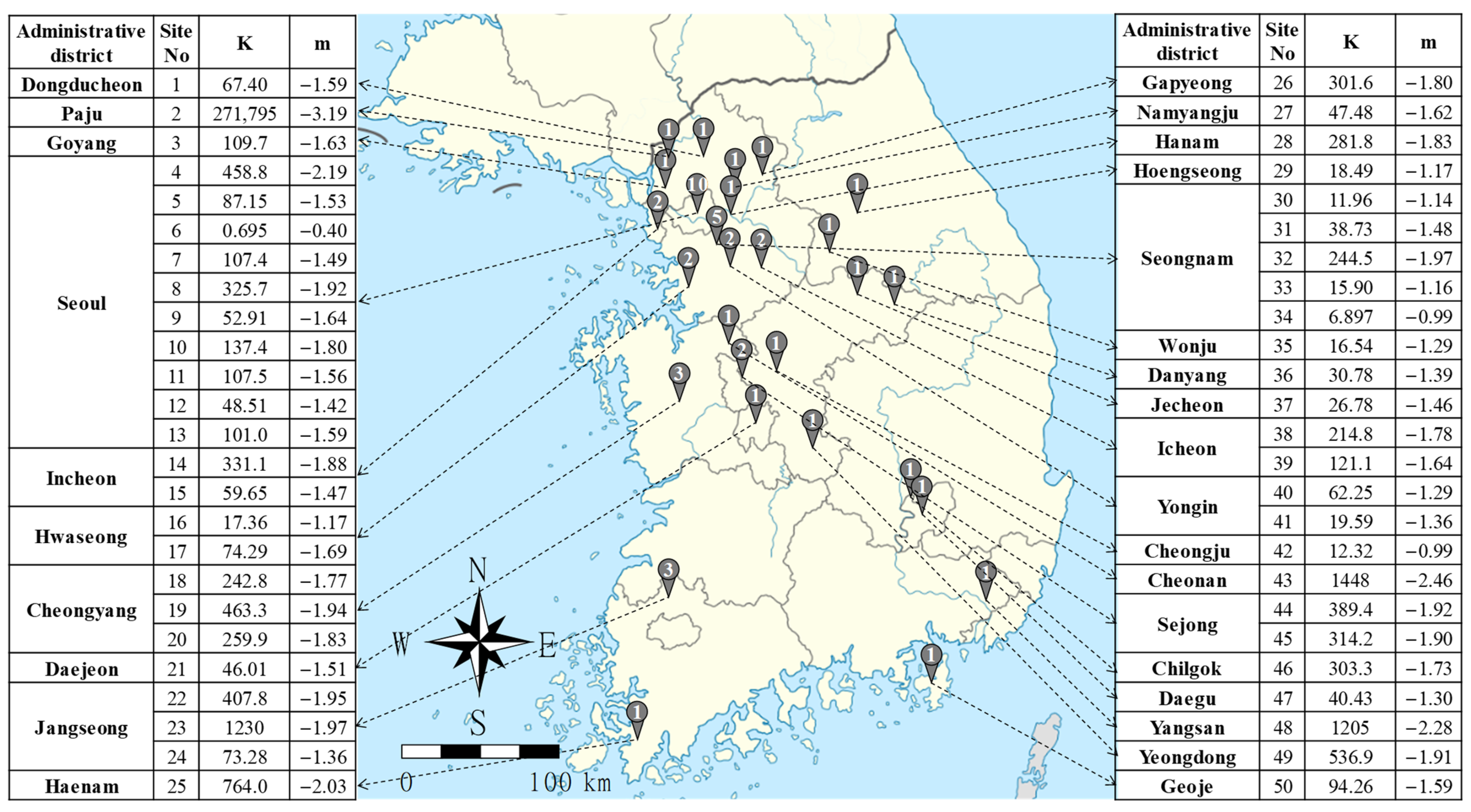
The authors collected 1191 blasting datasets, which are more than six times the datasets used in the previous studies, from 50 diverse construction sites, representing each region of South Korea. The locations of 50 diverse construction sites by 28 administrative districts are depicted in Figure 2. The number of construction sites that were conducted in the same administrative district is expressed in the circle. Even though the construction sites are located in the same administrative district, they are different construction sites. Building and road construction were the main site activities, and open-pit blasting was used at all 50 construction sites. Of the total 1191 datasets, 714 (60%) and 179 (15%) were used for prediction model development as training and validation datasets, respectively. The remaining 298 (25%) were used to test the models. The datasets were randomly designated for Training, Validation, and Testing via PYTHON code.
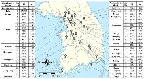
Figure 2.
Locations of 50 diverse construction sites by administrative district.
Predicting PPV requires a selection of influential factors. Since this study aims to predict the PPV accurately and easily at any open-pit blasting site, the influential factors should not only affect the PPV but also be easily obtained by untrained field staff.
Eleven common initial influential factors satisfied these conditions from 1191 blasting datasets: type of explosive (TE), charge weight per delay (W), specific weight (SW), length of drilling hole (LH), the height of the bench (HB), burden spacing (BS), hole spacing (HS), type of rock (TR), the distance between blasting and monitoring points (D), site factor K, and site factor m. To use an influential factor as quantitative data, the TE and the TR must be converted to values that express the velocity of detonation (VoD) and the velocity of the P-wave (VoP). The explosive types used at the 50 sites were Megamex, New emulate, Newmite, and Lovex manufactured by Hanwha Corporation [21]. The eight types of rock were gneiss, granite, limestone, schist, shale, andesite, rhyolite, and tuff. The conversion values are summarized in Table 1 and Table 2.
It is necessary to remove or change the initial influential factors to avoid multicollinearity that negatively affects prediction due to the high correlations between independent variables [22]. As shown in Figure 3, factors W, LH, HB, BS and HS are strongly correlated (>0.88) with each other. To remove a strong correlation between influential factors, we removed the LH, HB, BS and HS since W is the most important factor to PPV among the five factors. Finally, we selected seven influential factors relevant to PPV. The units and ranges of the selected factors and PPV are shown in Table 3.
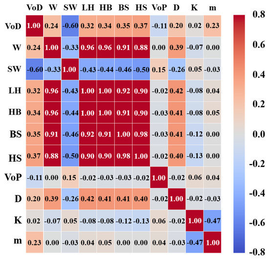
Figure 3.
Correlations between initial influential factors.

Table 1.
Input values for types of explosive.
Table 1.
Input values for types of explosive.
| Explosive Type | Megamex | New Emulite | NewMITE | LoVEX |
| Velocity of Detonation (m/s) | 6000 | 5900 | 5700 | 3400 |
Table 2.
Input values for types of rock.
Table 2.
Input values for types of rock.
| Rock Type | P-Wave Velocity (m/s) | Reference |
|---|---|---|
| Gneiss | 5500 | [23] |
| Granite | 5300 | [23] |
| Limestone | 5470 | [23] |
| Schist | 4550 | [23] |
| Shale | 3500 | [23] |
| Andesite | 5121 | [24] |
| Rhyolite | 4100 | [25] |
| Tuff | 2750 | [26] |
Table 3.
Characteristics of influential factors and peak particle velocity (PPV).
Table 3.
Characteristics of influential factors and peak particle velocity (PPV).
| Type | Parameters | Symbol | Unit | Range of Datasets |
|---|---|---|---|---|
| Input | Velocity of detonation | VoD | m/s | 3400–6000 |
| Charge weight per delay | W | kg | 0.1–10 | |
| Specific weight | SW | kg/m3 | 0.25–0.56 | |
| Velocity of P-wave | VoP | m/s | 2750–5500 | |
| Distance between blasting and monitoring points | D | m | 5–650 | |
| K | K | - | 0.7–271,795 | |
| m | m | - | −3.19 to −0.40 | |
| Output | Peak Particle Velocity | cm/s | 0.005–6.514 |
4. Prediction Models
4.1. Artificial Neural Network
Trial-and-error analysis of hyper-parameters is required to obtain the optimal prediction model which has the lowest validation loss. In this analysis, it was carried out with a different number of hidden layers, nodes, normalization methods, and activation functions; one and two hidden layers; 3, 5, 7, 11, 14, 15, 21, 28 and 35 nodes for the hidden layer; min-max and standard scalings; and three activation functions, sigmoid, hyperbolic tangent, and ReLU. In other words, 54 (2 × 9 × 3) and 486 (2 × 9 × 9 × 3) structures were assessed on 1 and 2 hidden layers, respectively. The number of nodes was determined by Table 4. Here, and mean number of input and output parameters, respectively. We added some equations in the final row of Table 4 to analyze many structures. The Adam optimizer [27] was used to reduce the loss with a learning rate of 0.001. Also, we used an early stopping to avoid overfitting and to obtain the best-fitted model. Every structure of the ANN model was trained with the 714 training datasets and validated by the 179 validation datasets. Every ANN model was developed with the software PYTHON Version 3.7.6.
Table 4.
Equations for determination of the number of nodes.
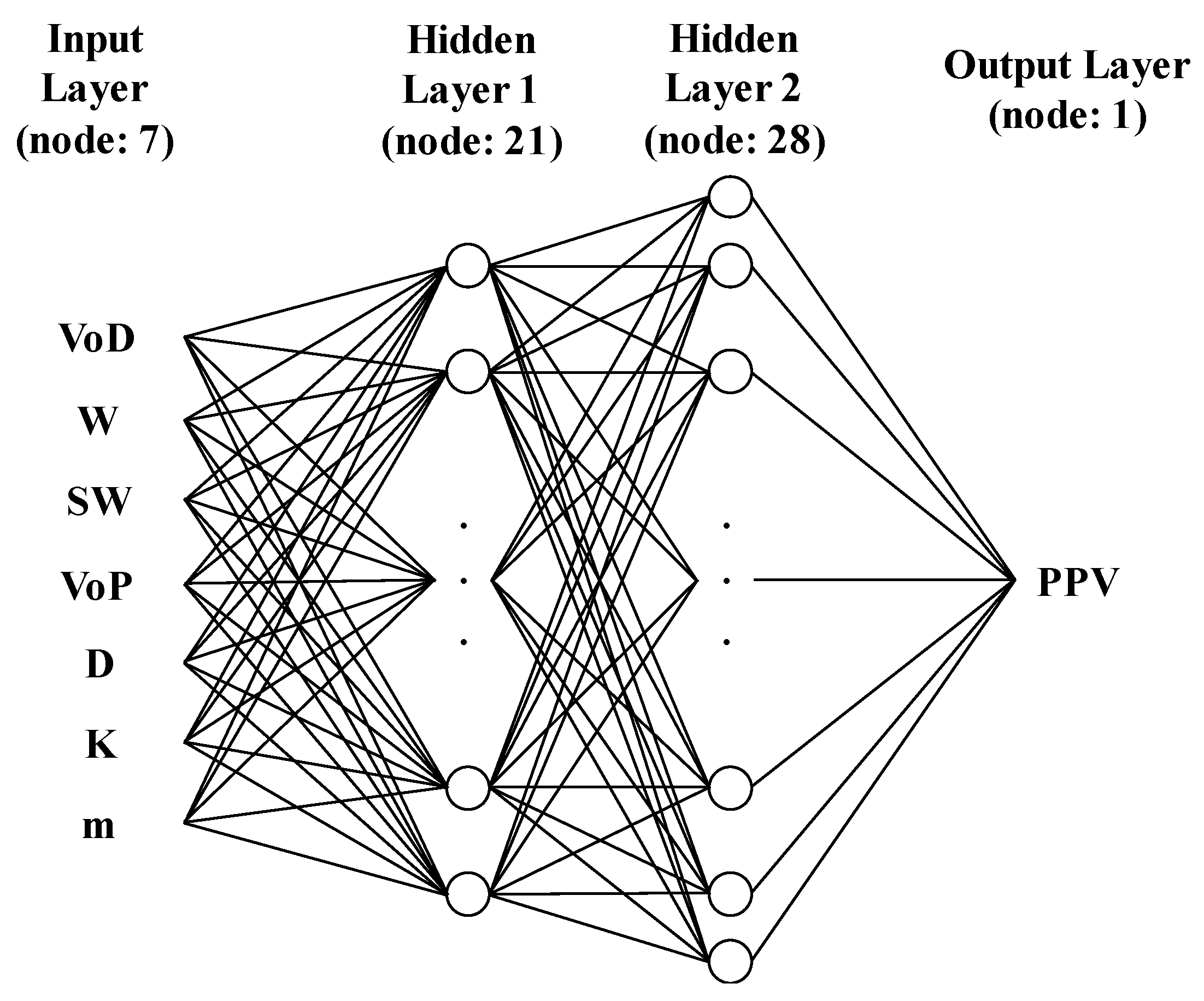
In the results of trial-and-error analysis, the average validation loss of 540 structures was 0.126 cm/s. Among the 540 ANN models, the structure composed of two hidden layers with 21 and 28 nodes, normalized by min-max scaling and combined with ReLU showed the lowest validation loss of 0.115 cm/s. Therefore, we selected the ANN model, which has the 7-21-28-1 structure depicted in Figure 4 as an optimal ANN model for a PPV prediction. The training of this model was stopped at 4208 epochs by early stopping. Table 5 summarizes the characteristics of the selected ANN model. This model is represented by Equations (10)–(12). PPV is calculated by Equation (10). Equations (11) and (12) represent hidden layers 1 and 2, respectively.
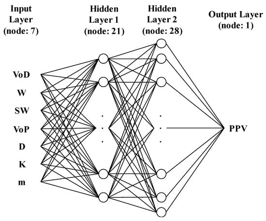
Figure 4.
Structure of the artificial neural network (ANN) model developed.
Table 5.
Characteristics of the ANN model.
In these equations, [I] is the matrix of input data sets, [W] is the matrix of weights, and [b] is the matrix of biases. The weight and bias matrices are constants that were obtained from the ANN training. Here, [], [], [], [], [], and [] are 7 21, 21 28, 28 1, 1 21, 1 28, and 1 1 matrices. When predicting i PPVs, [I] is an i 7 matrix. R is a ReLU function expressed by Equation (3), m is a min-max scaling expressed by Equation (4).
4.2. Empirical Formula
Each empirical formula of the 50 construction sites was generated using Equation (6) with the site factors, K and m. For instance, Equation (13) represents the empirical formula of Site 1 with K and m values of 67.4 and −1.59, respectively. The site factors of each site are represented in Figure 2. Through this method, 50 empirical formulas were generated and defined as EF-1. Each of the formulas included in EF-1 can only be applied to the PPV prediction at the site where it was generated. The K of Site 2, which is far higher than the rest, seems to be noise. In geotechnical engineering, some noise could have happened due to uncertainties. Thus, datasets obtained from Site 2 should also be analyzed with other datasets.
Test blasting is required to obtain site factors K and m, used in empirical formulas such as EF-1. However, it is difficult to perform test blastings at the preliminary design stage, and representative values of K and m are needed to compensate for this weakness. Representative K and m values of 200 and −1.6 were proposed based on Design and Construction Guidelines for Open-pit blasting in Road construction published by the Ministry of Land, Infrastructure, and Transport in South Korea [33]. We defined Equation (14) as EF-2 using the K and m. Many engineers have designed preliminary blasting patterns, applying Equation (14).
To derive one representative empirical formula for the 50 sites, we calculated K and m values of 74.9 and −1.535 using datasets of 50 open-pit blasting construction sites. Equation (15) expresses the representative empirical formula and it was defined as EF-3. Since this is a representative equation of 50 sites, it will show lower prediction accuracy than EF-1. However, it could be used at the preliminary design stage like EF-2. Figure 5 shows EF-3 (solid line) and the 893 datasets (circles) on a log-log plot where the vertical axis is PPV and the horizontal axis is SD. As mentioned in Section 2.2, EF-3 was obtained from the linear regression of the 893 blasting datasets.
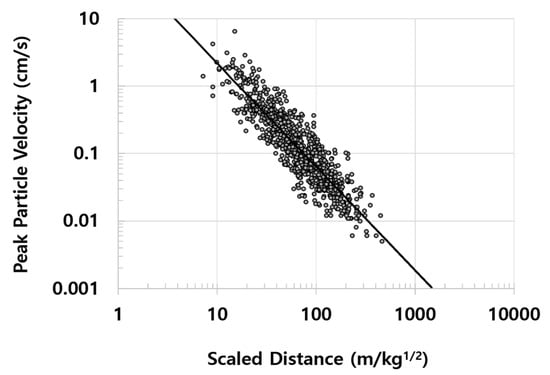
Figure 5.
Peak particle velocity versus scaled distance for 893 datasets.
Equations (16) and (17) are prediction models proposed by the International Society of Explosives Engineers (ISEE) [34] and USBM [35], respectively. These two equations have been widely used to predict PPVs. We defined Equations (16) and (17) as the ISEE model and USBM model, respectively.
4.3. Multivariable Regression Analysis
Multivariable regression analyses were carried out using IBM SPSS Statistics Version 26.0 (SPSS), which is a powerful statistical software package [36] that generates a simple equation for estimating output. Many researchers have performed multivariable regression analyses with ANN to compare the performance of prediction methods [15,16,37]. In this study, two types of multivariable regression analysis were carried out using training and validation datasets from 50 open-pit blasting construction sites to identify linear or non-linear relationships between influential factors and PPV. One was multivariable linear regression analysis (MLRA) and the other was multivariable non-linear regression analysis (MnLRA). The developed MLRA is represented by Equation (18). From seven influential factors, SW and VoP were excluded, since their partial regression coefficients had higher p-values than the significant level, 0.05. After the two factors were removed, the F and p-values of the MLRA model showed approximately 49 and 0, respectively. In addition, constant and five influential factors had p-values that were near 0. These F and p-values mean that the MLRA model is statistically significant. However, this model showed a low R of 0.495. The developed MnLRA is represented by Equation (19). This equation has been developed in exponential form following the form of the conventional empirical formula. p-values of all partial regression coefficients except for VoP were shown to be lower than the significant level, 0.05. Therefore, we removed the VoP from the input parameters. F and p-values of the MnLRA model showed approximately 898 and 0, respectively. Besides, the R of this model was high, 0.927. Here, the influential factor m was converted to –m in Equation (19) because all influencing factors and PPV are positive, while m is negative.
PPV = −0.588 + 1.2 × 10⁻⁴VoD + 0.092W − 0.003D − 1.45 × 10⁻⁶K − 0.193m
PPV = 0.034VoD0.79W0.741 SW−0.37D−1.602K0.375 (−m)−2.248
Note that test datasets were never used prior to the performance evaluation of the prediction methods. This means only the training and validation datasets were used to develop the ANN model, EF-1, 2 (K and m), MLRA, and MnLRA.
5. Prediction Results
5.1. Performance Comparisons of the Six Prediction Models
The 298 test datasets, which account for 25% of the total datasets obtained, were predicted using the eight predictive analysis methods, ANN, EF-1, EF-2, EF-3, ISEE model, USBM model, MLRA, and MnLRA, described in Chapter 4. First, the PPVs were predicted using the weights and biases matrices of the optimal ANN model. Here, all seven influential factors, VoD, W, SW, VoP, D, K, m were used as input parameters. Second, we used EF-1 which grouped 50 empirical formulas to predict PPVs of the test datasets. Here, each test dataset was predicted by the empirical formula of the site where they were obtained. W and D were used as input parameters. Finally, the test datasets were predicted by EF-2, 3, ISEE model, USBM model, MLRA, and MnLRA expressed as Equations (14)–(19), respectively, using input parameters of each method. In this study, three performance indicators, mean absolute error (MAE), root mean square error (RMSE), and mean absolute percent error (MAPE), were used to analyze prediction results. These performance indicators are listed in Table 6.
Table 6.
Equations of performance indicators.
Here, and are the i-th measured and predicted values, respectively, and n is the total number of test datasets. Table 7 summarizes the performances of the eight prediction models on the predicted PPVs. The developed ANN model achieved the lowest MAE of 0.064 cm/s, RMSE of 0.161 cm/s, and MAPE of 23.2%. These results were approximately 30%, 56%, and 11% lower than those from EF-1, which is currently the most commonly used method to predict PPVs when designing blasting patterns for construction. However, the EF-2 deduced the highest MAE of 0.305 cm/s and RMSE of 0.731 cm/s.
Table 7.
Performances of the six prediction models.
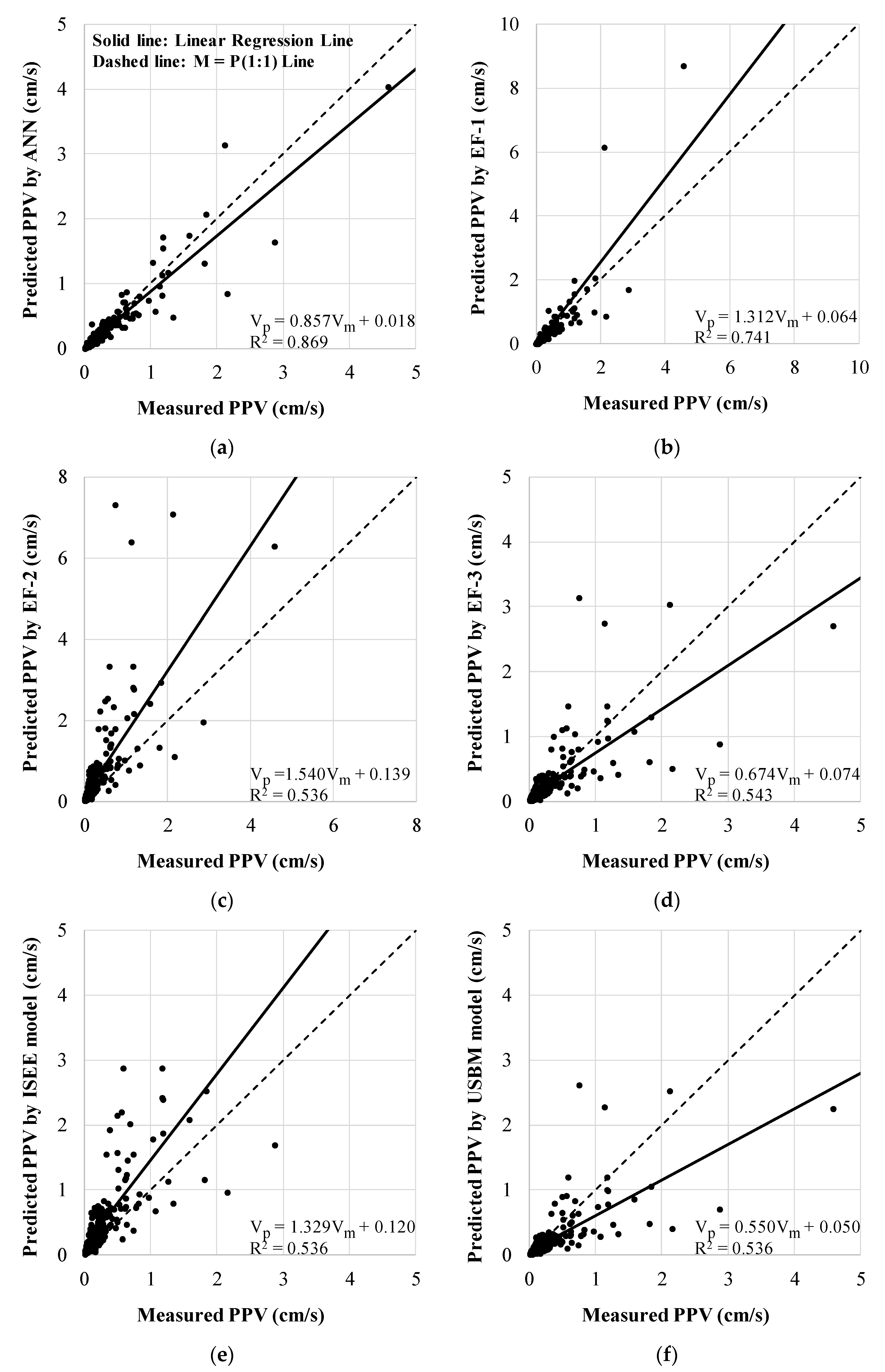
Linear regression analyses were performed with a coefficient of determination known as to explain the correlation and similarity between the predicted PPVs from the six predictive analysis methods and measured PPVs of the test datasets. The value of can be found using Equation (20), where and are measured and predicted PPV values, Cov is the covariation between two factors, and Var is the variation of a factor.
Each predicted PPV by the six prediction methods is plotted as a small circle in Figure 6a to 6h respectively according to prediction methods. The x and y axes represent the measured and predicted PPV, respectively, in cm/s. There are two lines in each figure. The dashed line is the Measured PPV = Predicted PPV (1:1) line and the solid line is the linear regression line. In the lower right corner of each figure, it shows the equation of the linear regression line and R2. The linear regression line resulting from the ANN shows the best result in terms of similarity to the 1:1 line as shown in Figure 6. The linear regression line resulting from the MLRA displays the greatest distance between the two lines.
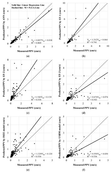
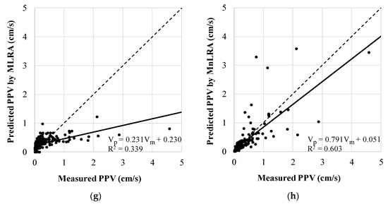
Figure 6.
Predicted PPV versus measured PPV by the six prediction methods. The graphs in (a–h) were made using predicted PPVs by the ANN, EF-1, EF-2, EF-3, ISEE model, USBM model, MLRA, and MnLRA, respectively.
5.2. Sensitivity Analysis
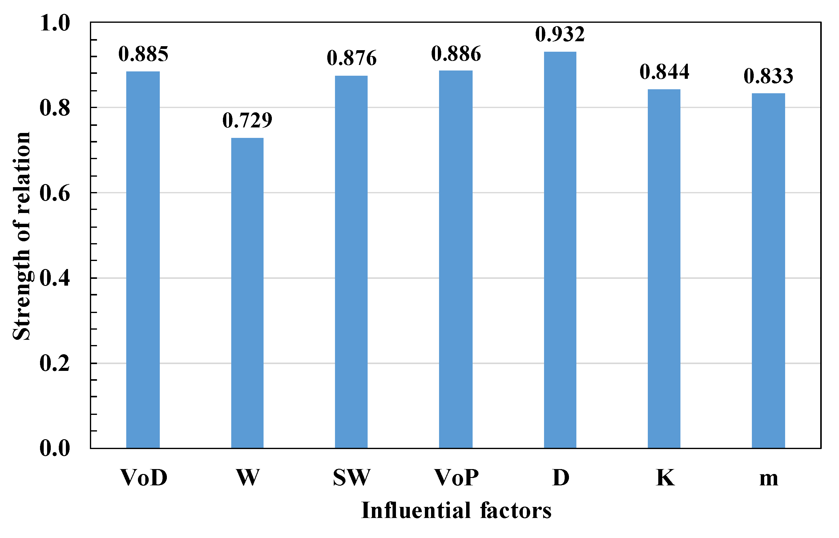
A sensitivity analysis was performed using the cosine amplitude method for all seven influential factors. This method has been applied previously [4,15,38] to determine the relative significance of each factor on PPV. It calculates a relation, , and provides results from a pairwise comparison of two factors, and , using Equation (21) [39].
The influential factors and PPV of the 1191 datasets, which consist of both training and test datasets, were logged and analyzed using Equation (21). The relative significances of the seven influential factors are depicted in Figure 7. The relative significances between VoD, W, SW, VoP, D, K, m, and PPV were deduced to be approximately 0.885, 0.729, 0.876, 0.886, 0.932, 0.844, and 0.833, respectively.

Figure 7.
Sensitivity analysis of the influential factors.
6. Discussion
The ANN model showed the best agreement with measured PPVs among eight prediction methods, including the globally used ISEE and USBM models. It would be due to using the most influential factors, which has the ability to reproduce and model the non-linear connections between input and output parameters, and to deal with noise. As shown in Figure 7, the seven influential factors have similar strengths of relation. It indicates that using these seven factors is more effective than using the only four factors which are included in the conventional empirical formula to predict PPVs. The complex connections between PPV and influential factors could be found in the comparison between the MLRA and MnLRA. When we developed these two models, they showed a statistical significance; however, the MLRA had a low R (0.495) while the MnLRA had a high R (0.927). The MAE from the MLRA showed about twice that of the MnLRA. These two models differ in their use of linear and non-linear relationships to explain PPV from influencing factors. Because of this difference, the MnLRA showed better predictive performance than the MLRA. It means that the relationships between the influential factors and PPV are non-linear. The ability to deal with noise could be verified by the prediction results about the biggest measured PPV, 4.58 cm/s, which is over 17 times the average measured PPVs, 0.26 cm/s. The prediction results from the ANN, EF-1, EF-2, EF-3, ISEE model, USBM model, MLRA, and MnLRA were 4.04, 8.7, 6.3, 2.72, 5.43, 2.25, 0.81 and 3.45 cm/s, respectively. The prediction results from the ANN model showed the closest to the measured PPV. It implies that the ANN has an excellent ability to deal with noise.
EF-2 showed the worst performances at MAE and RMSE and it would be due to its applicability. EF-2 is suitable for road construction sites because it was developed using only blasting datasets from road construction sites. These results mean that applying the conventional representative formula for a preliminary blasting design from road constructions has a limitation in applying it to other open-pit blastings. Therefore, a new alternative prediction equation is required. EF-3 which was developed using datasets from 50 diverse open-pit blasting construction sites would be suitable as the alternative prediction equation since it has the same form as EF-2, and it showed better predictive performances than EF-2.
The proposed model has been applied only to open-pit blasting construction sites. Future studies of PPV prediction models such as ANN model and EF-3 will include blasting records from underground caverns, tunnels, and mines as well to ensure the prediction models be generally applicable to any region and type of blasting.
7. Conclusions
In this study, the prediction of PPV using eight predictive analysis methods of ANN, EF-1, EF-2, EF-3, ISEE model, USBM models, MLRA, and MnLRA with 1191 datasets, which are more than six times the maximum datasets used in the previous studies, was carried out to assess PPV prediction methods at an open-pit construction site.
Seven key factors relevant to PPV were considered in the prediction models. The seven key factors were selected according to the ease of obtaining them and their influence on PPV. They consist of three factors, VoD, SW, and VoP, newly proposed in this study, and four key factors, W, D, and the site factors K and m, currently included in the conventional empirical formula. The use of three additional influential factors played a significant role in identifying the prediction model that produced the lowest error. Their significant roles were confirmed through a comparison of the performances of the ANN and others. These roles were also apparent in the results of the sensitivity analysis. The seven key factors have similar strengths of relations with PPV. It implies that not only are the previously used factors important in predicting PPV but also the newly added factors.
The PPV prediction based on the ANN model achieved the lowest values at MAE, RMSE, and MAPE among the eight prediction models. Even the ANN, which was generalized for application to all sites, produced lower errors than those from the EF-1, which can apply to only a specific site. In addition, the prediction accuracy of the ANN model was higher than that of the ISEE and USBM models. It would be attributed to the ability of ANN to express complex and non-linear relationships between influential factors and PPV, and the ability of ANN to deal with noise. It is necessary to perform a grid search for structures and hyper-parameters and early stopping to obtain an optimal prediction model. In this study, we compared 540 ANN models, to which were applied the early stopping method. These models have one or two hidden layers with the number of nodes calculated using the number of input and output parameters and three activation functions. Finally, a structure consisting of two hidden layers with 21 and 28 nodes using a ReLU as an activation function was determined as the optimal model. Other hyper-parameters were chosen following the previous studies. As a result, we generated the prediction model showing the lowest errors among the six prediction methods. Therefore, we recommend using an ANN for predicting PPVs whose hyper-parameters are selected from a grid search and literature research.
The EF-2 was proposed by the Ministry of Land, Infrastructure, and Transport in South Korea for designing preliminary blasting patterns. However, the MAE, RMSE, and MAPE associated with the EF-2 were over two times higher than those associated with the EF-3, which is newly proposed in this study. This difference might be a result of different construction types in the datasets. EF-3 was developed by analyzing data from 50 open-pit construction sites, including building construction sites in downtowns, road construction sites, aggregate extraction sites, and restoration work sites while EF-2 was developed by analyzing only datasets at road construction sites. Using the newly proposed EF-3, which proposes a K value of 74.9 and an m value of −1.535, for a preliminary design of open-pit blasting would be more accurate and reliable than using the EF-2.
The ANN model with the seven key factors and EF-3, proposed in this paper, can predict PPVs more accurately and will help blasting pattern design to be more reliable. The reliable blasting patterns will reduce environmental problems significantly and maximize the efficiency of blasting in construction. Moreover, the use of the newly proposed prediction methods will lessen civil complaints, and improve the efficiency in the construction schedule, and reduce the overall construction budgets. These advantages will lead to greater safety and sustainable urban development.
Author Contributions
Data curation, Y.-H.C.; Formal analysis, Y.-H.C.; Investigation, Y.-H.C.; Methodology, Y.-H.C.; Project administration, Y.-H.C.; Validation, Y.-H.C.; Writing—original draft preparation, Y.-H.C.; Conceptualization, S.S.L.; Funding acquisition, S.S.L.; Project administration, S.S.L.; Supervision, S.S.L.; Writing—review & editing, S.S.L. All authors have read and agreed to the published version of the manuscript.
Funding
This work is supported by the Korea Agency for Infrastructure Technology Advancement (KAIA) grant funded by the Ministry of Land, Infrastructure and Transport (Grant 21UUTI-B157786-02).
Institutional Review Board Statement
Not applicable.
Informed Consent Statement
Not applicable.
Data Availability Statement
Not applicable.
Acknowledgments
This work was supported by the Korea Agency for Infrastructure Technology Advancement (KAIA) grant funded by the Ministry of Land, Infrastructure and Transport (Grant 21UUTI-B157786-02) and by the National Research Foundation of Korea (NRF) grant funded by the Korea government (MSIT) (NRF-2020R1A6A3A13077513).
Conflicts of Interest
The authors declare no conflict of interest. The funders had no role in the design of the study; the collection, analyses, or interpretation of data; the writing of the manuscript; or the decision to publish the results.
References
- National Environmental Dispute Resolution Commission. Statistical Data, Such as Handling Environmental Disputes (31 December 2020). Available online: https://ecc.me.go.kr/front/user/main.do (accessed on 15 February 2021).
- German Standards Organization. DIN 4150-3: Structural Vibration—Part 3: Effects of Vibration on Structures; Deutsches Institut für Normung e.V.: Berlin, Germany, 1999. [Google Scholar]
- Siskind, D.E.; Stagg, M.S.; Kopp, J.W.; Dowding, C.H. Structure Response and Damage Produced by Ground Vibration from Surface Mine Blasting; US Department of the Interior, Bureau of Mines: New York, NY, USA, 1980.
- Hajihassani, M.; Armaghani, D.J.; Monjezi, M.; Mohamad, E.T.; Marto, A. Blast-induced air and ground vibration prediction: A particle swarm optimization-based artificial neural network approach. Environ. Earth Sci. 2015, 74, 2799–2817. [Google Scholar] [CrossRef]
- Duvall, W.I.; Petkof, B. Spherical Propagation of Explosion-Generated Strain Pulses in Rock; US Department of the Interior, Bureau of Mines: New York, NY, USA, 1959.
- Liu, Q.; Li, N.; Duan, J.; Yan, W. The Evaluation of the Corrosion Rates of Alloys Applied to the Heating Tower Heat Pump (HTHP) by Machine Learning. Energies 2021, 14, 1972. [Google Scholar] [CrossRef]
- Perera, A.; Azamathulla, H.; Rathnayake, U. Comparison of different Artificial Neural Network (ANN) training algorithms to predict atmospheric temperature in Tabuk, Saudi Arabia. Mausam 2020, 71, 551–560. [Google Scholar]
- Ahmadi, M.; Naderpour, H.; Kheyroddin, A. ANN Model for Predicting the Compressive Strength of Circular Steel-Confined Concrete. Int. J. Civ. Eng. 2016, 15, 213–221. [Google Scholar] [CrossRef]
- Kim, M.-S.; Lee, J.-K.; Choi, Y.-H.; Kim, S.-H.; Jeong, K.-W.; Kim, K.-L.; Lee, S.S. A Study on the Optimal Setting of Large Uncharged Hole Boring Machine for Reducing Blast-induced Vibration using Deep Learning. Explos. Blasting 2020, 38, 16–25. [Google Scholar]
- Nguyen, H.; Drebenstedt, C.; Bui, X.-N.; Bui, D.T. Prediction of Blast-Induced Ground Vibration in an Open-Pit Mine by a Novel Hybrid Model Based on Clustering and Artificial Neural Network. Nat. Resour. Res. 2019, 29, 691–709. [Google Scholar] [CrossRef]
- Azimi, Y.; Khoshrou, S.H.; Osanloo, M. Prediction of blast induced ground vibration (BIGV) of quarry mining using hybrid genetic algorithm optimized artificial neural network. Measurement 2019, 147, 106874. [Google Scholar] [CrossRef]
- Bui, X.-N.; Choi, Y.; Atrushkevich, V.; Nguyen, H.; Tran, Q.-H.; Long, N.Q.; Hoang, H.-T. Prediction of Blast-Induced Ground Vibration Intensity in Open-Pit Mines Using Unmanned Aerial Vehicle and a Novel Intelligence System. Nat. Resour. Res. 2019, 29, 771–790. [Google Scholar] [CrossRef]
- Tufféry, S. Data Mining and Statistics for Decision Making; John Wiley & Sons: Chichester, UK, 2011. [Google Scholar]
- Singh, A.; Thakur, N.; Sharma, A. A review of supervised machine learning algorithms. In Proceedings of the 2016 3rd International Conference on Computing for Sustainable Global Development (INDIACom), New Delhi, India, 16–18 March 2016; pp. 1310–1315. [Google Scholar]
- Khandelwal, M.; Singh, T. Prediction of blast-induced ground vibration using artificial neural network. Int. J. Rock Mech. Min. Sci. 2009, 46, 1214–1222. [Google Scholar] [CrossRef]
- Monjezi, M.; Ghafurikalajahi, M.; Bahrami, A. Prediction of blast-induced ground vibration using artificial neural networks. Tunn. Undergr. Space Technol. 2011, 26, 46–50. [Google Scholar] [CrossRef]
- Kim, Y.; Lee, S.S. Application of Artificial Neural Networks in Assessing Mining Subsidence Risk. Appl. Sci. 2020, 10, 1302. [Google Scholar] [CrossRef] [Green Version]
- Lee, C.-W.; Park, S.-Y. Prediction of Blasting-induced Vibration at Sintanjin Area, Daejeonusing Borehole Test Blasting. J. Korean Soc. Agric. Eng. 2018, 60, 55–62. [Google Scholar]
- Morhard, R.C. Explosives and Rock Blasting; Atlas Powder Company: Wilmington, DE, USA, 1987. [Google Scholar]
- Suh, H.; Yang, K.; Kim, N.; Kim, H.; Kim, M. SPSS (PASW) Regression Analysis, 3rd ed.; Hannarae: Seoul, Korea, 2009. [Google Scholar]
- Hanwha Corporation. Hanwha Corporation Explosive Products Guide; Hanwha Corporation: Seoul, Korea, 2017. [Google Scholar]
- Matignon, R. Data Mining Using SAS Enterprise Miner; John Wiley & Sons: Hoboken, NJ, USA, 2007; Volume 638. [Google Scholar]
- Barton, N. Rock Quality, Seismic Velocity, Attenuation and Anisotropy; Taylor and Francis Group: London, UK, 2006. [Google Scholar]
- Fathollahy, M.; Uromeiehy, A.; Riahi, M. Evaluation of P-wave velocity in different joint spacing. Bollettino di Geofisica Teorica ed Applicata 2017, 58, 157–168. [Google Scholar]
- Mielke, P.; Bär, K.; Sass, I. Determining the relationship of thermal conductivity and compressional wave velocity of common rock types as a basis for reservoir characterization. J. Appl. Geophys. 2017, 140, 135–144. [Google Scholar] [CrossRef]
- Vinciguerra, S.; Trovato, C.; Meredith, P.; Benson, P.; Troise, C.; De Natale, G. Understanding the Seismic Velocity Structure of Campi Flegrei Caldera (Italy): From the Laboratory to the Field Scale. Pure Appl. Geophys. PAGEOPH 2006, 163, 2205–2221. [Google Scholar] [CrossRef]
- Kingma, D.P.; Ba, J. Adam: A method for stochastic optimization. arXiv 2014, arXiv:1412.6980. [Google Scholar]
- Kaastra, I.; Boyd, M. Designing a neural network for forecasting financial and economic time series. Neurocomputing 1996, 10, 215–236. [Google Scholar] [CrossRef]
- Sheela, K.G.; Deepa, S.N. Review on Methods to Fix Number of Hidden Neurons in Neural Networks. Math. Probl. Eng. 2013, 2013, 1–11. [Google Scholar] [CrossRef] [Green Version]
- Mamaqani, B.H.M.H. Numerical Modeling of Ground Movements Associated with Trenchless Box Jacking Technique; The University of Texas at Arlington: Arlington, TX, USA, 2014. [Google Scholar]
- Hecht-Nielsen, R. Kolmogorov’s mapping neural network existence theorem. In Proceedings of the International Conference on Neural Networks, San Diego, CA, USA, 21–24 July 1987; pp. 11–14. [Google Scholar]
- Hush, D.R. Classification with neural networks: A performance analysis. In Proceedings of the IEEE 1989 International Conference on Systems Engineering, Fairborn, OH, USA, 24–26 August 1989; pp. 277–280. [Google Scholar]
- The Ministry of Land, Infrastructure and Transport in Korea. Open-Pit Blasting Design and Construction Guideline for Road Construction. Available online: http://www.molit.go.kr/USR/BORD0201/m_34879/DTL.jsp?mode=view&idx=28896 (accessed on 23 February 2021).
- Hopler, R.B. ISEE Blasters’ Handbook; International Society of Explosives Engineers (ISEE): Cleveland, OH, USA, 1998. [Google Scholar]
- Nicholls, H.R.; Johnson, C.F.; Duvall, W.I. Blasting Vibration and Their Effects on Structures; US Department of the Interior, Bureau of Mines: New York, NY, USA, 1971.
- IBM SPSS Software. Available online: https://www.ibm.com/analytics/spss-statistics-software (accessed on 21 April 2021).
- Khandelwal, M.; Singh, T. Prediction of blast induced ground vibrations and frequency in opencast mine: A neural network approach. J. Sound Vib. 2006, 289, 711–725. [Google Scholar] [CrossRef]
- Monjezi, M.; Hasanipanah, M.; Khandelwal, M. Evaluation and prediction of blast-induced ground vibration at Shur River Dam, Iran, by artificial neural network. Neural Comput. Appl. 2012, 22, 1637–1643. [Google Scholar] [CrossRef]
- Ross, T.J. Fuzzy Logic with Engineering Applications; John Wiley & Sons: Chichester, UK, 2004. [Google Scholar]


Publisher’s Note: MDPI stays neutral with regard to jurisdictional claims in published maps and institutional affiliations. |
© 2021 by the authors. Licensee MDPI, Basel, Switzerland. This article is an open access article distributed under the terms and conditions of the Creative Commons Attribution (CC BY) license (https://creativecommons.org/licenses/by/4.0/).