Abstract
Omnidirectional honeybee traffic is the number of bees moving in arbitrary directions in close proximity to the landing pad of a beehive over a period of time. Automated video analysis of such traffic is critical for continuous colony health assessment. In our previous research, we proposed a two-tier algorithm to measure omnidirectional bee traffic in videos. Our algorithm combines motion detection with image classification: in tier 1, motion detection functions as class-agnostic object location to generate regions with possible objects; in tier 2, each region from tier 1 is classified by a class-specific classifier. In this article, we present an empirical and theoretical comparison of random reinforced forests and shallow convolutional networks as tier 2 classifiers. A random reinforced forest is a random forest trained on a dataset with reinforcement learning. We present several methods of training random reinforced forests and compare their performance with shallow convolutional networks on seven image datasets. We develop a theoretical framework to assess the complexity of image classification by a image classifier. We formulate and prove three theorems on finding optimal random reinforced forests. Our conclusion is that, despite their limitations, random reinforced forests are a reasonable alternative to convolutional networks when memory footprints and classification and energy efficiencies are important factors. We outline several ways in which the performance of random reinforced forests may be improved.
1. Introduction
Continuous electronic beehive monitoring (CEBM) uses various sensors to extract information on honeybee (Apis Mellifera) colony behavior and phenology. Automated video analysis is an important component of CEBM because it provides bee traffic assessment without much disturbance to colonies and reduces fatigue and transportation costs associated with human beehive monitoring. Unlike other methods used in CEBM (e.g., continuous weight monitoring or individual bee tagging), video methods are not as expensive and do not interfere with natural colony cycles.
We use the terms bee and honeybee interchangeably to refer to the Apis Mellifera honeybee and to no other bee species. We use the terms hive and beehive to refer to a Langstroth hive [1] hosting a live Apis Mellifera colony. We use the phrases omnidirectional bee traffic and omnidirectional traffic to refer to the number of bees moving in arbitrary directions in close proximity to the landing pad of a hive over a given period of time.
Bee traffic is an indicator of how bee colonies react to foraging opportunities, weather events, pests, and diseases. Commercial and amateur apiarists use bee traffic in proximity of hives to estimate the state of their colonies, because such traffic contains information on colony behavior. Bee traffic may also indicate colony exposure to stressors such as failing queens, predatory mites, and airborne toxicants.
In our previous article [2], we proposed a two-tier (2T) algorithm to measure levels of omnidirectional traffic in videos taken from the top of a hive. The algorithm combines class-agnostic motion detection with class-specific image classification. Tier 1 segments a video into frames and, in each frame, produces motion regions where moving objects may be present; tier 2 applies class-specific classifiers to the image regions from tier 1 to detect the presence or absence of specific objects (e.g., bees) in each region. The algorithm outputs a bee motion count (i.e., the number of motion regions classified as BEE) for each input video. In tier 1, we experimented with three motion detection algorithms: KNN [3], MOG [4], and MOG2 [5]. In tier 2, we used support vector machines (SVMs) [6], random forests (RFs) [7], and convolutional networks (ConvNets) [8].
In this article, we continue our systematic investigation of tier 2 classifiers for 2T video analysis of omnidirectional traffic. It is critical for video-based CEBM to find classifiers that approach the classification accuracy of ConvNets without requiring equally large memory footprints and power levels. Tier 1 methods are beyond the scope of this article.
Our article proceeds as follows. In Section 2, we review investigations directly relevant to our research and outline the contributions to video-based CEBM we make in this article. In Section 3, we describe the image datasets we used in our experiments. In Section 4, we define a random reinforced forest (RRF) as a random forest (RF) trained on a dataset with reinforcement learning (RL) [9] and present several RRF construction methods. In Section 5, we present our concept of shallow convolutional network (SCN): a convolutional network is defined as shallow, if its size on disk, after it is persisted, is smaller than a domain-dependent threshold in acceptable memory units. Our definition of shallowness is different from the definition of shallowness in the ConvNet literature where shallowness is defined in terms of the number of layers in a ConvNet (e.g., [10]). In Section 6, we develop a theoretical framework for the complexity analysis of image classification with SCNs and RFs. This analysis is fundamental not only to physical run-time performance of these classifiers, but also to their energy consumption. In Section 7, we describe our experiments with SCNs and RRFs on seven image datasets. In Section 8, we formulate and prove three theorems on finding optimal RRFs. These theorems provide a theoretical basis for explaining some experimental results. In Section 9, we discuss our findings and present our conclusions.
2. Related Work
Several investigations on video-based CEBM are related to our research. In this section, we briefly review these investigations and outline the contributions reported in this article.
Estivill-Castro et al. [11] present a color segmentation algorithm to track bees pollinating macadamia trees. The algorithm computes the absolute differences of the Minkowsky metric [12] between the R-, G-, and B-channels of consecutive frames. The researchers report that the Minkowsky metric shows greater differences when frames contain bees flying against clear, static background and smaller values with frames that contain bees flying behind flowers. The channel differences are used to detect flying bees. The researchers claim that their algorithm can detect motions of leaves and flowers. The proposed method does not distinguish small stigmas or vibrating leaves from bees or bees flying over flowers.
Kimura et al. [13] propose a vector quantization method to segment bee bodies in video frames. The methods identifies bee body regions with vector quantization. Two types of regions, named single honeybee region (SHR) and plural honeybee region (PHR), are extracted with morphological information such as body size and body shape. The method works on 30 frames per second (fps) videos with a resolution of 720 × 480 and is reported to detect over 500 bees per frame. In the reported experiments, the method successfully identified 72% of the bees. The proposed method appears to work best to track motions in large masses of bees inside the hive, not outside of it.
Chen et al. [14] propose a computer vision system to monitor the beehive’s in-and-out activity. The system uses an infrared LED camera, an infrared LED light source, and a personal computer to process images. A large sample of forager bees is captured and placed in a freezer where the bees are rendered temporarily motionless due to low temperature. A circular character encoding tag is glued to each motionless bee’s thorax. The tags are used to recognize the bees’ flight orientations in images. Hough transform [15] is used to detect tags and classify them with an SVM. The researchers report the orientation classification accuracy of ≈98% and claim that their method avoids the disadvantages of heavier RFID tags and does not require external readers emitting electromagnetic waves. Placing RFID tags on bees interferes with natural life cycles of bees and is not practical for commercial apiarists.
Ghadiri [16] proposes a video bee traffic monitoring system whose camera is placed in front of or on top of a hive. The system estimates bee traffic by detecting changes between the current image and the average image of the preceding eleven images. The change mask contains segments, each of which is assumed to correspond to a single bee. The sum of these segments constitutes a bee count. The reported research appears to offer insufficient detail on the accuracy of the proposed method.
Babic et al. [17] proposed a system for detecting pollen bearing honeybee in videos at the entrance of a hive. The system’s raspberry pi camera is placed in a box above the hive entrance. A glass plate is placed on the bottom side of the box, 2 cm above the landing pad. This configuration forces the bees entering or leaving the hive to crawl ≈11 cm. The training dataset consisted of 50 images of pollen bearing honeybees and 50 images of honeybees without pollen. The test dataset consisted of 354 honeybee images. Since the bees in the camera’s field of view cannot fly, the system’s design may interfere with natural bee cycles. The experimental results are not replicable insomuch as the test datasets do not appear to be public.
Rodriguez et al. [18] designed a system for pose detection and tracking of insects and animals. The researchers used their system to monitor the traffic of honeybees and mice. A deep neural network was trained to detect and associate body parts into whole insects or animals. The network returns a set of 2D confidence maps of present body parts and a set of vectors of part affinity fields. Greedy inference is used to compile the parts into larger insects or animals. Trajectory tracking is used to distinguish entering and leaving bees at smaller bee traffic levels. blueUnlike the datasets used in our investigation, the dataset used to evaluate the proposed system consisted of 100 fully annotated frames, where each frame contained 6–14 honeybees.
In this article, we contribute to the body of video-based CEBM research by presenting two methods of training RFs on image datasets with reinforcement learning (RL). We call these classifiers random reinforced forests (RRFs). RRFs can be used in the second tier of 2T algorithms to count omnidirectional bee motions in bee traffic videos. They can also be used in other video-based CEBM algorithms (e.g., [13]) that identify if a given region contains a bee before processing it with more sophisticated techniques. We compare the performance of RRFs with SCNs on seven image datasets.
Another contribution we make to video-based CEBM is a theoretical framework for assessing the complexity of image classification. This framework may appeal to machine learning (ML) researchers working on image classification. We formulate and prove three theorems on finding optimal RRFs. Our main finding is that, despite their limitations, RRFs present a reasonable alternative to ConvNets when memory footprints, image classification efficiency, and energy efficiency are important factors (e.g., in embedded systems with limited power supplies).
3. Image Datasets
In this section, we briefly describe the BEE1, BEE2_1S, BEE2_2S, and BEE3 datasets obtained in the course of our video-based CEBM research in 2014–2020, because these datasets were used in this investigation. We refer interested readers to our previous article [19] for details on how these datasets were curated. All images were obtained from 30 s 24-frames-per-second videos obtained with BeePi monitors deployed on live bee hives [2]. Each dataset is split into training, testing, and validation subsets. The training and testing datasets include the images used for model fitting (i.e., for training and periodically testing classifiers); the validation datasets include the images not used either in training or testing, but only in the final model selection.
BEE1 includes 54,391 images obtained in 2017. If an image contains at least one complete bee, it is labeled as BEE; if it contains no complete bee or only a small part of a complete bee, it is labeled as NO_BEE. The training dataset includes 19,082 (35%) BEE and 19,057 (35%) NO_BEE images; the testing dataset includes 6362 (12%) BEE and 6362 NO_BEE (12%) images; the validation dataset consists of 1801 (3%) BEE and 1718 (3%) NO_BEE images.
BEE2 contains 112 879 images obtained in 2018. We call a video 1-super when it is captured by a camera mounted on a hive that consists of one deep super. We refer to a video as 2-super when it is captured by a camera mounted on a hive that consists of two deep supers. BEE2 is split into two subsets: BEE2_1S (58,201 150 × 150 images) and BEE2_2S (54,674 90 × 90 images). All images are labeled as BEE or NO_BEE. In BEE2_1S, 8266 (14%) BEE and 27 108 (46%) NO_BEE images are selected for training; 2828 (5%) BEE images and 9035 (16%) NO_BEE images—for testing; and 8298 (14%) BEE images and 2666 (5%) NO_BEE images—for validation. In BEE2_2S, 12 982 (24%) BEE images and 15,983 (29%) NO_BEE images are for training; 4194 (8%) BEE images and 5327 (10%) NO_BEE images—for testing; and 6823 (12%) BEE and 9369 (17%) NO_BEE images—for validation.
BEE3 contains 65,023 64 × 64 images obtained in 2019. All images are labeled as BEE, NO_BEE, and SHADOW_BEE. The category SHADOW_BEE includes images that, in the judgment of a human classifier, contains shadows of bees. In BEE3, 12,948 (20%) BEE, 12,857 (20%) NO_BEE, and 12,006 (18%) SHADOW_BEE images were randomly selected for training; 4236 (7%) BEE, 4242 (6%) NO_BEE, and 3993 (6%) SHADOW_BEE—for testing; and 5187 (7%) BEE, 5204 (8%) NO_BEE, 4350 (8%) SHADOW_BEE—for validation. In this article, we refer to BEE3 datasets without SHADOW_BEE images as BEE3_NS (i.e., BEE3_NO_SHADOW), and to the complete BEE3 dataset with SHADOW_BEE images as BEE3_S (i.e., BEE3_SHADOW).
BEE4 is a new dataset which we have not previously published. This dataset was obtained from BEE2_2S in 2021 by re-labeling 996 (1.8%) images in BEE2_2S, because during a 2020 labeling verification a human evaluator decided that these images were mislabeled: some bee images were mislabeled as NO_BEE and some images with bee shadows were mislabeled as BEE. Table 1 shows the distribution of images in BEE4.

Table 1.
BEE4 image distribution per category.
We also used the CIFAR-10 dataset [8] to test our algorithms on a more general image dataset. CIFAR-10 consists of 60,000 color images distributed among 10 different classes. We used the testing subset of CIFAR-10 that includes 10,000 images with 1000 images per class for model selection, and randomly divided the training set into 40,000 training images (4000 images per class) and 10,000 testing images (1000 images per class) for model fitting.
4. Random Reinforced Forests
A random reinforced forest (RRF) is a random forest (RF) trained on a dataset with reinforcement learning (RL). RL involves an agent that executes a finite set of actions in an environment to learn which action to execute in which state of the environment. When an agent performs an action, it receives a positive or negative reward from an interpreter that executes the agent’s action in the environment, evaluates the next state of the environment, and gives the agent feedback according to a reward function. The agent is assumed to be interested in maximizing the reward.
In our case, the agent learns how to construct an RF for an image dataset. The agent’s actions are confined to adding different decision trees (DTs). A state of the environment is an RRF’s representation specifying which DTs the RRF contains. For example, if there are n DTs out of which the agent can construct RRFs, an RRF can be represented as a set of DT identifiers. Alternatively, it can be represented as a n-bit string where a 1 bit signals the presence of a corresponding tree and a 0-bit signals its absence. We combined the interpreter and the environment into a Python script that evaluates an RRF on a validation dataset and gives the agent feedback based on the RRF’s accuracy.
A DT in an RRF is uniquely determined by its depth (i.e., the length of the longest path from the root to a leaf) and its local receptive field (LRF). An LRF is an area in an image whose pixels a DT uses to classify images. Formally, a DT is denoted as , where refers to the DT’s LRF and is the DT’s depth. An RRF F of n DTs is a set of trees .
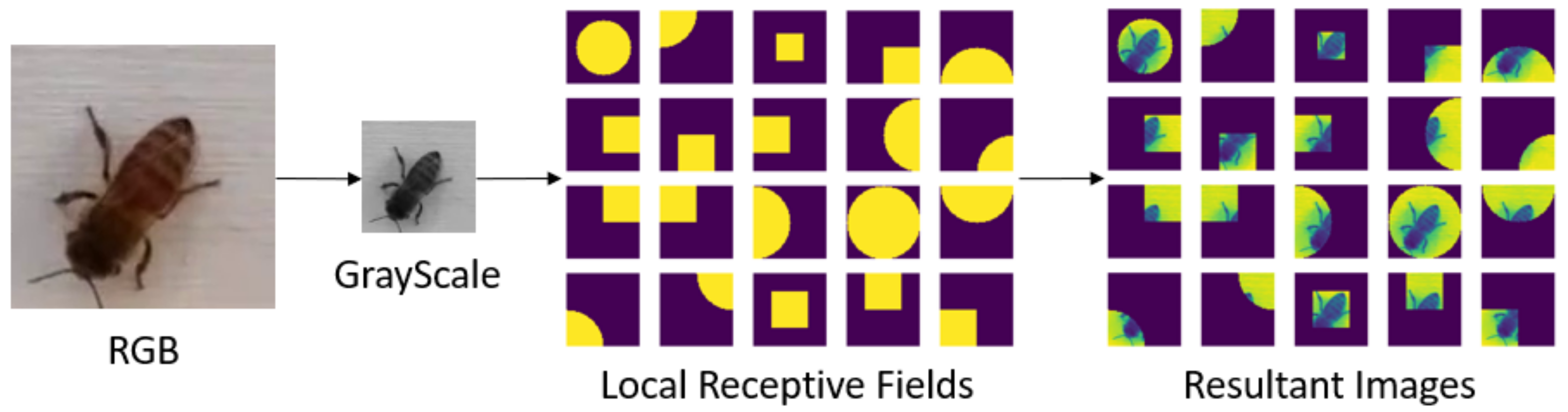
Figure 1 illustrates how we constructed LRFs for this investigation. All RGB images are grayscaled and resized to . We defined 20 different LRFs, each of which covers a specific area of the input image (See Local Receptive Fields in Figure 1). We refer to the process of superimposing an LRF on an image as LRF overlap. Although, in principle, LRFs may have arbitrary shapes, we confined our investigation to circles and squares of specific radii and side lengths. Given a radius of 32 and a side length of 32, a circle’s center and a square’s top left corner are shifted left to right across a image in increments of 16 pixels and their intersections with the image are taken to represent 9 LRFs defined by the intersections of the image with the shifting circle of radius 32 and another 9 LRFs defined by the intersections of the image with the shifting square with side 32. LRF 19 is the intersection between the image and the circle of radius 16 placed in the center of the image. LRF 20 is the intersection between the image and the square with side 16 placed in the center of the image. Each LRF, when overlapped with an image, may contain a whole bee, part of a bee, or no bee (See Resultant Images in Figure 1).
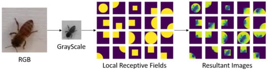
Figure 1.
LRF construction: (1) RGB image is grayscaled; (2) 20 LRFs are overlapped with grayscale image.
4.1. RRF Construction
Bootstrap aggregation is a process of randomly picking n samples with replacement from a dataset. These n in-bag samples are used to train one DT. An RRF is an ensemble of multiple DTs trained through bootstrap aggregation (aka bagging) of samples.
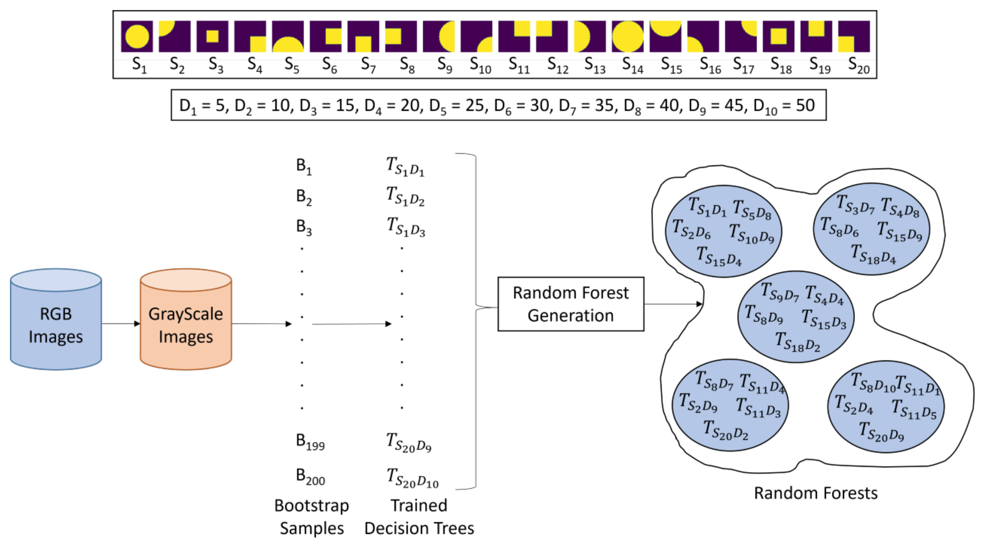
Given an image dataset, our RRF construction algorithm generates 200 bootstrap samples {}. There are 20 LRFs {} and 10 predefined depths measured in pixels , where and , . All 200 possible DTs are trained on the bootstrap samples. The trained DTs are persisted and used by the algorithm to construct RRFs. The total number of possible RRFs, excluding the empty one, that can, in principle, be constructed is . Figure 2 shows how RRFs are constructed with the RL methods explained in Section 4.2 below.

Figure 2.
RRF construction with hidden Q-learning (HQL) and dynamic Q-learning (DQL) described in Section 4.2.
4.2. Hidden and Dynamic Q-Learning
Q-Learning is an RL algorithm used in many ML applications. This algorithm starts with the initialization of the so called Q-Table (aka the Q-Matrix) with 0’s. The Q-Table rows are the states of the environment and the columns are the actions that the agent can execute. Each cell in the Q-Table specifies the cumulative reward (aka q-value) the agent receives if it executes the corresponding action in the corresponding state.
The agent chooses an action by means of (1) exploitation (i.e., the maximum value in the current row is chosen and the action specified by the corresponding column is executed) or (2) exploration (i.e., a random action is chosen). The extent of exploration and exploitation is controlled by the parameter (aka the -value). The greater the -value, the higher the degree of exploration. A best practice is to aggressively explore early on and gradually switch to exploiting the acquired knowledge later (i.e., gradually decay from 1 to 0).
After the agent takes an action a in a state s and receives a reward r, the entry for s and a in the Q-Table (i.e., ) is updated according to Equation (1), where is the learning rate, is the discount factor, and is the maximum Q-value over all possible actions available to the agent in the next state to which the environment transitions after a is executed in s.
We designed two Q-Learning methods (hidden Q-Learning (HQL) and dynamic Q-Learning (DQL)) for our RRF construction algorithm. Both methods take as input a list of DTs trained on bootstrap samples from a given dataset. Specifically, both methods are given a list of 200 DTs trained on 200 bootstrap samples from a given dataset. The trained DTs are enumerated from 1 to 200.
In HQL, the agent has 200 actions (i.e., , , ..., ), where , , denotes adding the k-th trained DT to a given RRF. There are 200 states (i.e., , , ..., ), each of which specifies the DT last added to the RRF. Thus, signals that DT 1 is last added to the RRF; signals that DT 2 is last added to the RRF, etc. Equivalently, we can interpret to mean that the RRF contains at least one instance of k-th DT. The initial state is chosen by randomly selecting integer k from [1, 200] and adding the k-th DT to the initially empty RRF. We called this method HQL, because the RRF itself is not explicitly specified in the Q-Table (i.e., it is a hidden variable); the RRF is used by the algorithm to compute action rewards every time a DT is added to it.
HQL runs for 1000 episodes with 100 steps each. These numbers are arbitrary and can be increased or decreased as required. At each step of an episode, after a DT is added to the RRF, the RRF’s validation accuracy is evaluated and the reward is computed as the difference of the current validation accuracy and the previous validation accuracy. The initial validation accuracy is set to the validation accuracy of the initial RRF (i.e., the accuracy of its only randomly selected DT) and becomes the previous validation accuracy. The current validation accuracy is recomputed after the addition of each new DT to the RRF. If at some step of an episode, the RRF’s validation accuracy is ≥90%, RL stops and the RRF is constructed from the Q-Table and persisted. Appendix A.1 gives a step-by-step example of how HQL method works to construct an RRF out of four DTs.
In DQL, the states are represented as 200-bit vectors. If bit k is toggled, the k-th DT is in the RRF; if bit k is untoggled, the k-th DT is not in the RRF. The initial state is a 200-bit vector where a randomly selected bit is toggled. The DQL agent also has 200 actions (i.e., , , ..., ), where , , denotes adding the k-th DT to a given RRF. However, the RRF is not hidden insomuch as each state (i.e., row) in the Q-Table explicitly specifies an RRF. We called this method DQL, because the initial Q-Table contains exactly one row; the other rows are added dynamically during RL.
DQL runs for 1000 episodes with 100 steps each. At each step of an episode, after a DT is added to the RRF, the RRF’s validation accuracy is evaluated. The DQL reward is computed either as (1) the difference of the current validation accuracy and the previous validation accuracy or as (2) the difference between the current validation accuracy and a given validation accuracy threshold. We refer to DQL where reward is computed according to rule 1 as DQL 1 and to DQL where reward is computed according to rule 2 as DQL 2. The initial validation accuracy is set to the validation accuracy of the initial RRF with one randomly chosen DT and becomes the previous validation accuracy in the next iteration. The current validation accuracy is recomputed after the addition of each new DT to the RRF. As in HQL, if at some step of an episode, the validation accuracy of the RRF is ≥90%, RL stops and the RRF is constructed from the Q-Table and persisted. Appendix A.2 gives a step-by-step example of how DQL method works to construct an RRF out of four DTs in two episodes to show learning transfer (i.e., access to previous states).
Since DQL runs for 1000 episodes, each of which has 100 steps, the total number of states that can theoretically be explored by DQL is . However, if DQL explores (i.e., visits) all these states, there is no knowledge transfer from previous states. To estimate the amount of knowledge transfer from previous states, we executed 26 experiments with DQL 1 and 26 experiments with DQL 2. Each experiment consisted of a method (i.e., DQL 1 or DQL 2) executed for 1000 episodes with 100 steps each, as described above. In each experiment, we recorded the number of states in each Q-Table and computed the maximum, the minimum, and the mean number of states across all experiments. Each row in Table 2 records these numbers.
Table 2.
DQL state visitation experiments on all seven image datasets (BEE1, BEE2_1S, BEE2_2S, BEE3_S, BEE3_NS, BEE4, CIFAR-10); Min is minimum number of states in Q-Table in all experiments; Max is maximum number of states in Q-Table in all experiments; Mean is mean number states in Q-Table in all experiments; Mean % Revisit shows mean percent of states that are revisited; DQL method is described in Section 4.1.
The state re-visitation statistics (in %) are shown in the last column of Table 2. Each revisitation statistic is computed as (Mean—100,000)/100,000. For example, the DQL 1 revisitation statistic is (78,630–100,000)/100,000 . The mean revisitation statistic for for DQL 1 and DQL 2 is , which indicates that not all possible states (i.e., 100,000 states) are explored and knowledge transfer from previous states does take place.
5. SCNs
A convolutional network (ConvNet) is said to be shallow, if its size on disk, after it is persisted, is , where is an application-dependent threshold measured in acceptable memory units (e.g., MB). Given a dataset, we define a ConvNet to be a shallow ConvNet (SCN) for the dataset if its memory footprint is less than or equal to the footprint of the largest RRF trained on the same dataset. In our investigation, we set MB, because the memory footprints of all trained RRFs for all datasets we used in our comparative experiments described below (i.e., BEE1, BEE2_1S, BEE2_2S, BEE3, and BEE4, and CIFAR) had a median footprint of 50 MB.
The SCN architecture we used in this study is shown in Figure 3. In addition to the input and output layers, the architecture consists of a convolutional layer (CL), max-pooling layer (MPL), and a fully connected layer (FCL). We fixed the node activation function to ReLU and incremented the number of filters in the CL and MPL and the number of nodes in the FCL until the persisted trained SCNs (i.e., instances of the SCN architecture) satisfied the shallowness criterion to have the memory footprint of ≤50 MB.
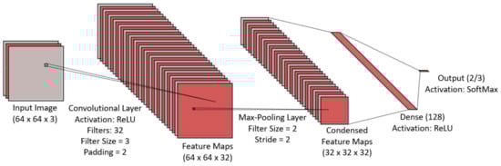
Figure 3.
SCN architecture used in this investigation.
6. Complexity Analysis of Image Classification with RRFs and SCNs
Image classifiers are typically compared in terms of accuracy, precision, recall, F-1, and ROC curves, etc. The complexity analysis of image classification by various trained classifiers remains relatively unexplored. Yet, this type of analysis is fundamental not only to physical run-time performance, but also to energy consumption [20]. In this section, we define a theoretical framework for doing the complexity analysis of image classification with SCNs, RFs, and RRFs. In our analysis, we assume that number addition, subtraction, multiplication, division, and comparison are performed in constant time. For example, the activation of ReLU, which is the maximum of 0 and the output, requires 2 operations, because it is one if-then-else statement.
6.1. RRFs
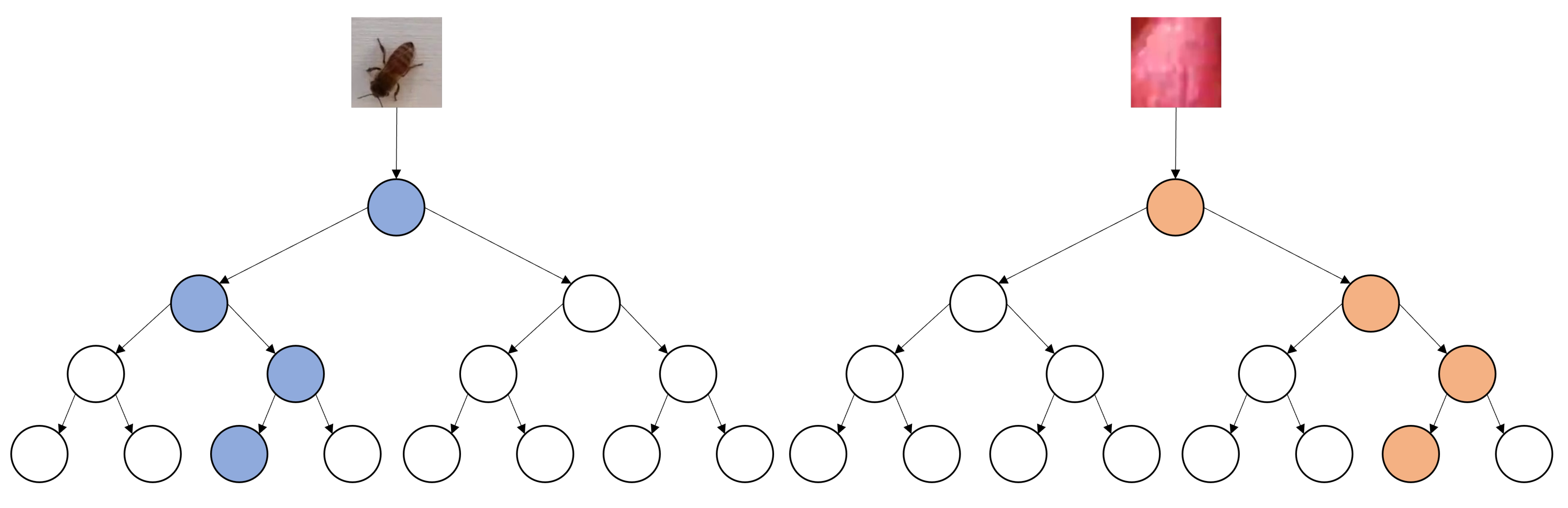
A DT is a full binary tree of height H. If each node involved in classifying a given image is a parameter, then the maximum number of nodes involved in the classification of single image is equal to exactly H (See Figure 4). Each DT has a specific LRF overlapped with an image before the actual classification along a specific path begins. If and denote the height and width of the input image, then the number of parameters used in its classification is , in the worst case.

Figure 4.
Number of DT parameters in classification of single image.
A trained DT T is a full binary tree of height H. Thus, the maximum number of nodes in T is . When T is used as an image classifier it thresholds exactly one pixel value along a specific path from the root to a leaf to determine the class of the image. Since thresholding requires 2 basic operations, the total number of operations T takes to classify an image is , because at each node along the path a threshold decision is made on the value of a single pixel to go left or right (See Figure 4).
Let us assume that an RRF F contains n DTs each of which has been trained to classify images into C classes with a specific LRF. Given an input image (i.e., of height h and width w), for each DT in F, the image is overlapped with the DT’s LRF. To perform the overlap, each pixel in the image is checked to see if it is present in the LRF’s pixels, which requires operations. LRF overlapping is analogous to masking, because all pixels covered by the LRF retain their original values, whereas all other pixels are set to 0. If F contains n DTs, the number of overlap operations is .
After LRF overlapping is done, F classifies the masked image with each , , to obtain n probability lists , where contains C probabilities computed by the corresponding as the proportion of the training data covered by ’s leaf node reached on the input image from its root along a specific path (See Figure 4). The mean probability of each class, i.e., , is computed, which requires additions and 1 division, and the maximum is returned.
If the maximum DT height in F is , then, in the worst case, the number of operations required to classify an image with F, , is given in Equation (2).
6.2. SCNs
As shown in Figure 3, we assume that an SCN consists of an input layer (IL), a convolutional layer (CL), a max pooling layer (ML), and a fully connected layer (FC), which coincides with the output layer (OL). The SCN uses ReLU as the activation function for all nodes.
Let the input dimensions to the CL be and suppose that the CL has filters, each of which has dimensions . The formula for the total number of parameters in the CL, , is given in Equation (3) as the sum of the numbers of the shared weights in the filters and the number of biases, the latter being equal to the number of the filters.
The ML does not add any additional parameters, because the feature maps obtained from the CL are downsampled, i.e., converted into the feature maps of lower dimensions with such functions as maximum, mean, etc.
Let the FC have input nodes and suppose the number of nodes in the FC itself is . The total number of parameters in the FC, , is given in Equation (4) as the sum of the number of weights connected between the layers and and number of biases.
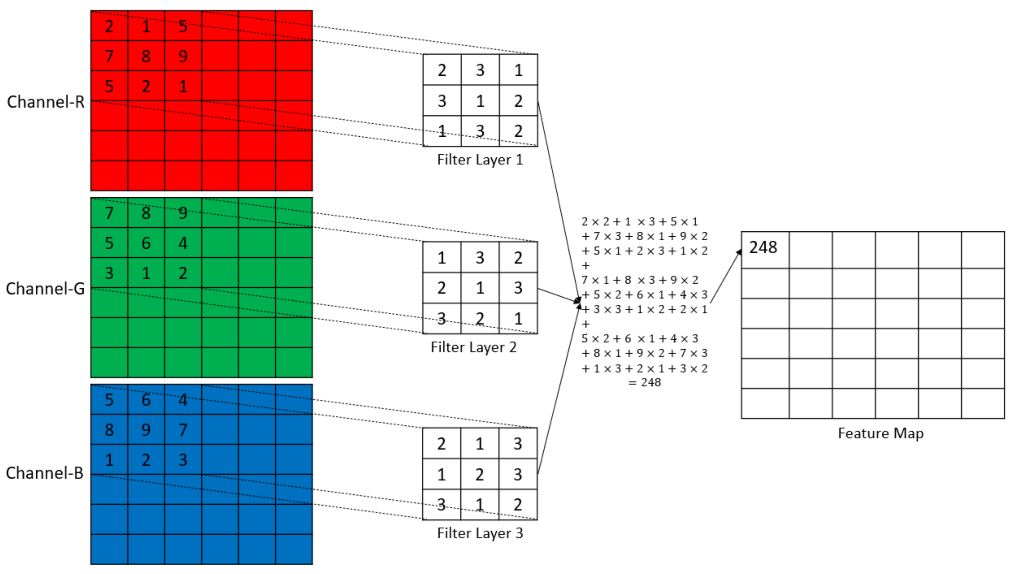
Let the input dimension to the convolutional layer be and use filters, where each filter’s dimensions are . A single convolution contains multiplications while the filter is overlapped with the LRF, additions to sum the multiplications, 1 bias addition, and 2 operations for ReLU activation. Thus, there are operations in a single convolution (See Figure 5). The total number of operations happening in the CL, , for an output size of is shown in Equation (5).

Figure 5.
Graphic representation of convolution.
Let the input dimension to the ML be and let the filter dimensions be . In a single max-pooling operation, there are a maximum of operations (See Figure 6). The total number of operations happening in the OL, , for an output size of is given in Equation (6).
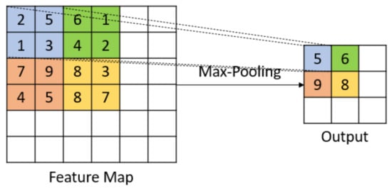
Figure 6.
Graphic representation of max-pooling.
Let the number of input nodes to the FL be and the number of nodes in the fully connected layer be . For a single node in the FL, there are multiplication to multiply the inputs and the respective weights, additions to compute the sum of the input and weight multiplications, 1 bias addition, a maximum of 2 operations for ReLU activation. Thus, there are operations for a single node in the FL. The total number of operations happening in in the FL, , is given in Equation (7).
Let the number of nodes in the FL be and number of nodes in the output layer (number of classes) be . The activation used in the output layer is softmax which calculates the probabilities based on the weighted output calculated before the activation. In addition to the operations happening for the multiplications and additions, there are operations to sum all weighted outputs, operations to normalize the weighted outputs and operations to calculate the maximum activation to define the class of the input. The total number of operations in the OL, , is given in Equation (8) and the total number of operations in the SCN, , is given in Equation (9).
7. Experiments and Results
In this section, we describe our experiments with six different models on the datasets. The best validation accuracies of the various methods on each of the datasets are reported in Table 3. The six classification models we used in our experiments are described below.
Table 3.
Validation accuracies (in %) of classifiers on all datasets; SKL_RF is scikit-learn RandomForestClassifier trained on grayscale images; SKL_RFC is the scikit-learn RandomForestClassifier trained on color images; BEE3_NS is BEE3 dataset with SHADOW_BEE images removed; BEE3_S is BEE3 dataset with SHADOW_BEE images; green cells indicate best accuracies.
The first classifier is the HQL RRF. We performed a grid search of values of 0.7, 0.8, and 0.9 and values of 0.1, 0.2, and 0.3. The value was updated by the the rule after each learning episode. The Q-Matrix obtained with the HQL method is used to generate the sequence S of DTs to generate the RRFs. Initially, S contains the 2 DTs that correspond to the state and action of the maximum q-value in the Q-Matrix. After the addition of the 2 DTs, the Q-Matrix cell with the maximum q-value is set to zero and the reconstruction recursively continues from the last action performed. Recall that the last action specifies the number of the last DT added. Specifically, the reconstruction goes to the corresponding state and performs the action of adding the DT whose number is specified in the column of the maximum q-value for the row. After the DT is added, the Q-Matrix cell with the maximum q-value is set to 0. The process continues until the number of the added DTs reaches 200. The HQL RRF was trained on the grayscaled images of all datasets.
Let be the sequence of DTs added to the RRF according to the maximum q-values in the Q-Matrix. In other words, is added first, then , etc. After the addition of each DT , the validation accuracy of the RRF, were it to be constructed from the DTs in S, is computed. Thus, if the initial sequence S contains , then the validation accuracy of the RRF that contains only is computed and recorded. If is the second DT in S, then the validation accuracy of of the RRF that contains is computed and recorded. Formally, the sequence is computed, where is the subsequence of S that starts with and ends with . The HQL RRF is constructed from the pair , where is the maximum of . Put another way, the HQL RRF is constructed from the minimal subsequence of DTs in that has the maximum validation performance.
The second and third classifiers are the the DQL 1 and DQL 2 RRFs. We performed a grid search of values of 0.8, and 0.9 and values of 0.1 and 0.2. The value was updated by the the rule after each learning episode. The DQL 1 and DQL 2 RRFs were trained on the grayscaled images of all datasets.
We call the fourth classifier the performance RF (PRF). To generate the PRF, the trained DTs are sorted in the descending order of their validation accuracies. Let this sequence be , where is a DT and is the maximum validation accuracy and is the minimal accuracy. The sequence is used in construction of the PRF in the same way as the sequence is used in the construction of the HQL RRF. Put another way, the PRF is constructed from the minimal subsequence of DTs added in the order of the DTs in that has the maximum validation performance. The PRFs were trained on the grayscaled images of all datasets.
The fifth classifier is the base case random forest classifier constructed with the RandomForestClassifer class of the scikit-learn library [21]. For each dataset, we trained the RFs with 50, 100, and 150 DTs using the Gini function both on the color and grayscale images of each dataset. These classifiers were trained on both grayscaled and color images of all datasets.
The sixth classifier is the SCN in Figure 3. We trained this architecture on the training and testing data of each dataset and persisted all trained models. A grid search of the parameters such as learning rate, weight decay, and dropout percentage was performed on each dataset. In the grid search, the learning rate was confined to the values 0.001, 0.01, and 0.1; the L2 weight decay was confined to 0.0001, 0.001, 0.01, and 0; the dropout was confined to 0, 0.2, 0.3, 0.4, and 0.5.
The model training used the model checkpoint to save the best model based on the lowest testing loss in all epochs. All SCNs were trained on the color images of all datasets.
The validation accuracies for the overall best models for each dataset are given in Table 3. While the SCNs performed better than the RRFs on four datasets BEE1, BEE2_1S, BEE3_NS, and BEE3_S, the RRFs outperformed the SCNs on the more challenging datasets BEE2_2S and BEE4. These datasets are more challenging, because the camera is positioned above the second super of the Langstroth beehive. Thus, the average number of pixels per honey bee is smaller. The HQL and DQL 2 RRFs performed on par on all datasets, except for BEE2_2S, where DQL 2 slightly outperformed HQL. The performance of the DQL 1 RRFs was the worst on all datasets. On CIFAR-10, SCNs outperformed all RFs: the performance of the SCN exceeded the performance of SK_RFC by 18.45% and the performance of the HQL RRF by 23.95%.
It is instructive to inspect the validation accuracy curves of the HQL RRFs and PRFs on various datasets with the values of and parameters (See Equation (1)) used in the grid search. Figure 7 indicates that on BEE1 all RFs kept improving performance until the number of the DTs in them reached 30, after which their validation accuracy varied between 90% and 95%. The PRF’s accuracy reached its peak performance of 91% when the number of DTs in it was 20, after which it started slowly declining until its number DTs exceeded 75, after which the rate of decline accelerated.
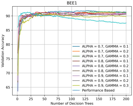
Figure 7.
Validation accuracy (in %) vs. number of DTs of HQL RRFs and PRF on BEE1.
Figure 8 indicates that on BEE2_1S, as the number of DTs in the HQL RFs was increasing, their accuracy was varying between 68% and 70%. The accuracy of the PRF was highest when the number of DTs in it was 5 and then kept declining. The BEE2_1S validation curves suggest that for this dataset, the RFs with smaller numbers of DTs performed better in that their validation accuracy was above 70% and, in the case of the PRF, reached 80%.
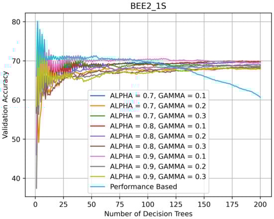
Figure 8.
Validation accuracy (in %) vs. number of DTs of HQL RRFs and PRF on BEE2_1S.
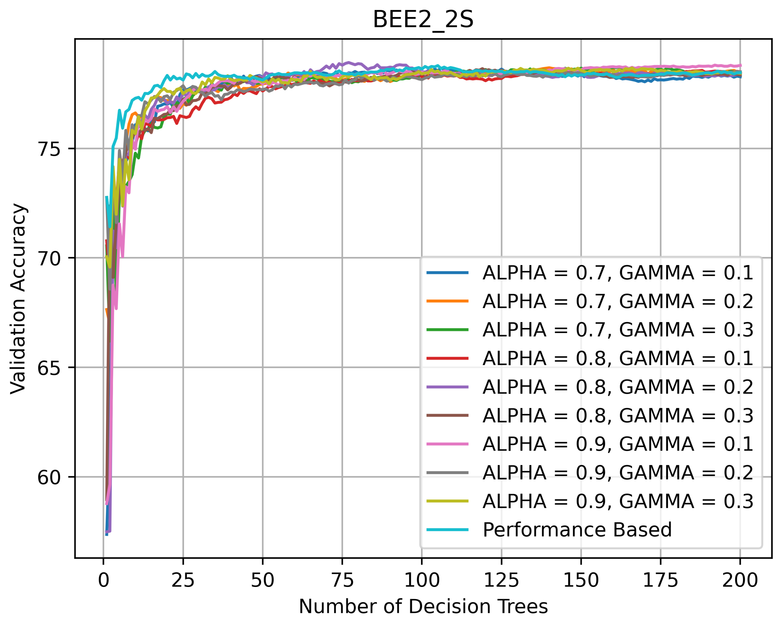
On BEE2_2S (see Figure 9), one of the two most challenging datasets, all RFs kept improving their performance until the number of DTs in them reached 100, after which their accuracy stabilized around 78%. The PRF’s accuracy did not decline with the addition of new DTs.

Figure 9.
Validation accuracy (in %) vs. number of DTs of HQL RRFs and PRF on BEE2_2S.
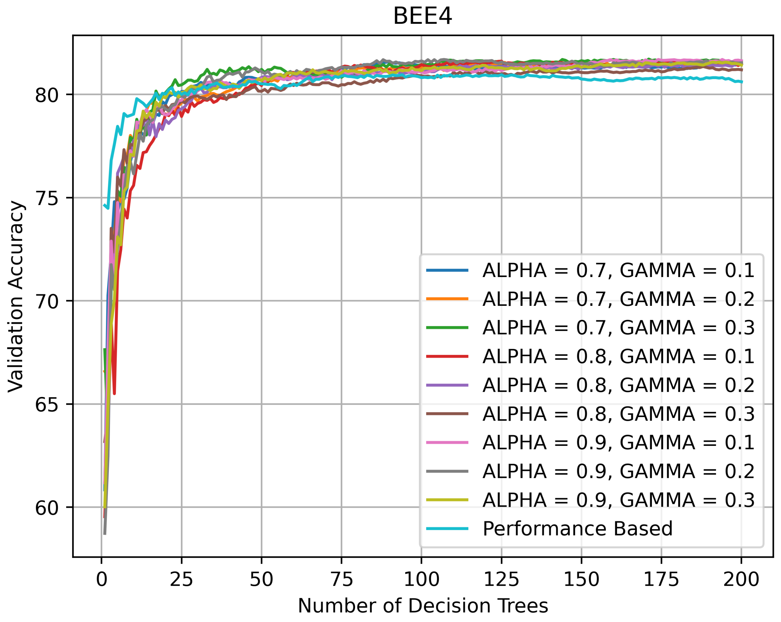
On BEE4 (see Figure 10), the second of the two most challenging datasets, the topology of the validation curves is similar to the topology on BEE2_2S. All RFs kept improving their performance until the number of DTs in them reached 100, after which their accuracy stabilized around 82%. The PRF’s accuracy did not decline as rapidly as on BEE1 and BEE2_1S with the addition of new DTs, but showed a slight decline after the number of DTs exceeded 125.
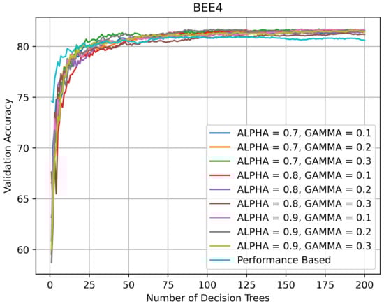
Figure 10.
Validation accuracy (in %) vs. number of DTs of HQL RRFs and PRF on BEE4.
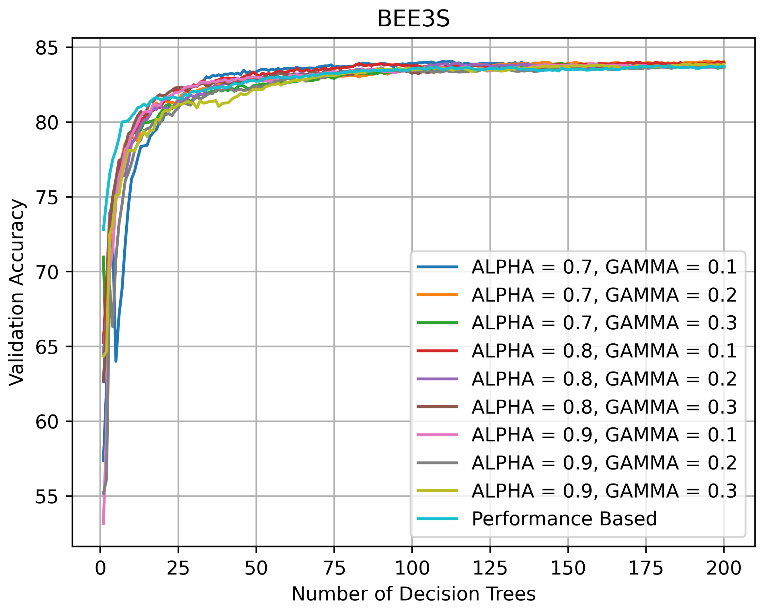
On BEE3 (see Figure 11 and Figure 12), the topology of the validation curves was similar. The accuracy spread was wider on BEE3 without SHADOW_BEE images after the number of DTs exceeded 50 and the accuracy varied between 85 and 87%. The accuracy spread was narrower on BEE3 with SHADOW_BEE images after the number of DTs exceeded 50 and the accuracy stayed at ≈83%.
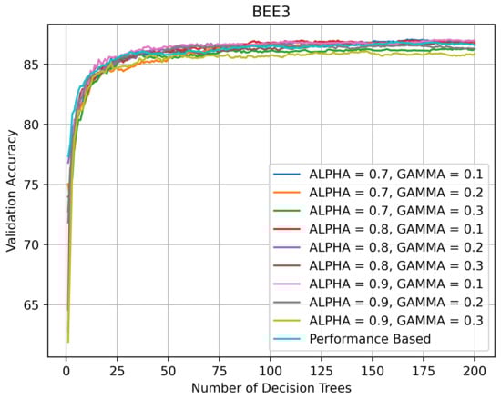
Figure 11.
Validation accuracy (in %) vs. number of DTs of HQL RRFs and PRF on BEE3_NS.
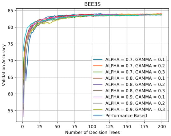
Figure 12.
Validation accuracy (in %) vs. number of DTs of HQL RRFs and PRF on BEE3.
One reason for the relative underperformance of DQL RRFs, especially DQL 1 RRFs, is the difficulty in finding optimal RRF with DQL, which we formulated and proved as Random Reinforced Forest Theorem 1 (RRFT 1) in Section 8 below. Another reason for the better performance of the SCNs may be their over-parameterization of the problem space [20], which allows them to generalize better with multiclass datasets that have relatively small numbers of training examples in each class. As the accuracies in the SKL_RF and SKL_RF (Color) indicate, the addition of color to images did not improve the performance of the scikit-learn RFs.
8. Random Reinforced Forest Theorems
In this section, we formulate three theorems on finding optimal RRFs for various datasets. These theorems provide a theoretical basis for explaining some experimental DQL results reported in Section 7. The proofs of these theorems are given in Appendix A.3 for readers interested in technical details.
Let {, , , ..., } be the set of trained DTs using k bootstrap samples from a dataset. There are possible RFs. Since each RF is a possible state in the DQL, the maximum number of possible states, M, is . An RRF is said to be a optimal random forest if and only if its performance (i.e., validation accuracy) is greater than a given threshold (e.g., ). In the theorems below, we use the terms random forest and state interchangeably, because in DQL, each state (i.e., a row in the Q-Table) corresponds to exactly one random forest and vice versa.
Theorem 1 (Random Reinforced Forest Theorem 1 (RRFT 1)).
Let M be a total number of possible RFs (i.e., possible states), of which B are optimal. If (i.e., B is considerably small than M), then the probability of not finding any optimal RRF with DQL is ≈1.
An immediate corollary of this theorem is that the probability of not finding any optimal state in N trials, , is
If we assume that there is at least one optimal state, given a set of DTs, out of which RRFs are constructed, i.e., , then is
Thus, if there are 200 DTs, out of which RRFs can be constructed, then and , . Is there such a value of for which the probability of not finding any optimal RRF in N trials is ≈0? The next theorem gives an answer to this question.
Theorem 2 (Random Reinforced Forest Theorem 2 (RRFT 2)).
Let , where B is the number of optimal states (i.e., optimal RFs) and N is the number of trials (i.e., the number of explorable states in DQL). Then, if N and M are large, the probability of not finding any optimal state is
As a function of B, increases as B decreases. The third theorem answers the question, what is the threshold for B that makes the probability of finding at least one optimal RRF less than 50%.
Theorem 3 (Random Reinforced Forest Theorem 3 (RRFT 3)).
Let M be a total number of possible RFs (i.e., possible states), of which B are optimal. Let N be the number of explored states in DQL (i.e., the number of trials) such that . There exists a threshold value x for B that makes the probability of finding at least one optimal RRF less than 50%.
If there are 200 DTs, then and , then the threshold is ≈ (See Equation (A6)). Thus, even if we have a large numberof optimal RRFs, the probability of not finding any optimal RRF is greater 50%.
9. Discussion and Conclusions
The SCNs performed better on four bee datasets BEE1, BEE2_1S, BEE3_S, BEE3_NS with validation accuracies of 97.0%, 89.16%, 90.52%, 88.08%, respectively. The datasets BEE2_2S and BEE4 are more challenging than the other bee datasets, because the images are taken from videos captured by the camera positioned above the second deep super of the Langstroth beehive, which makes individual bees smaller (in terms of the average bee size in pixels). On these two datasets BEE2_2S and BEE4, all RRFs, except for the DQL 1 RRF, performed better than the SCNs.
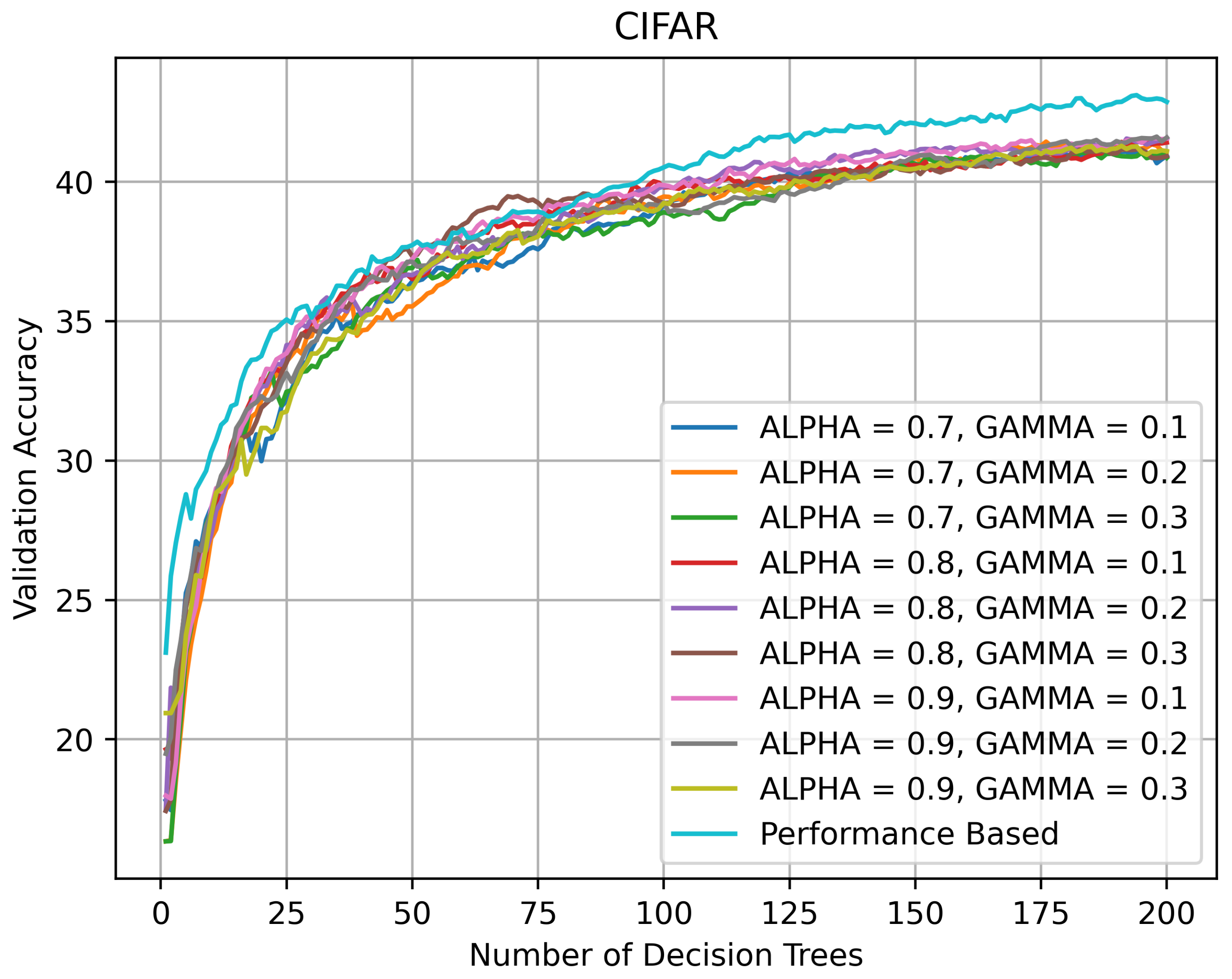
On CIFAR-10, the SCNs outperformed all RRFs, which indicates that on datasets with multiple categories and small numbers of images per category, the SCNs may generalize better than RRFs. As shown in Figure 13, all RRFs (except DQL 1) performed in the same ballpark of ≈43% on CIFAR-10. while the best SCN had an accuracy of 65.56%. Another possible implication is that on datasets such as CIFAR-10 it is the over-parameterization of the problem space [20] typical of convolutional networks that allows them to generalize better, although it is possible that a different set of LRFs may allow them to generalize better.

Figure 13.
Validation accuracy (in %) vs. number of DTs of HQL RRFs and PRF on CIFAR-10.
The importance of constrained grid search is an important lesson that we learned during the development of the SCNs. While we knew that grid search is a best practice in many ML domains including deep learning [22], initially, we tuned the hyper-parameters and changed the SCN architecture manually, which was neither systematic nor optimal in terms of performance. After switching to constrained grid search (i.e., finite sets of learning rates, weight decays, and dropouts), we were able to improve the SCN classification accuracies much faster. We also observed that systematically changing the hyperparameters gave us better results than tinkering with the SCN architecture.
The physical training time for the SCNs varied between 30 and 40 min per model per dataset. In contrast, the physical time for constructing an RRF was ≈10 h per dataset, most of which was consumed by RL. To understand this time difference, we need to look no further than the RL reward calculation, which was the largest bottleneck in our experiments. At each step of HQL or DQL, the reward is based on the validation accuracy of a specific RRF, which, in turn, depends on the size of the validation dataset of a given dataset. Put another way, the RRF must classify each image in the validation dataset after the addition of every DT.
On the other hand, the trained RRFs are much faster in classifying images at run time than the SCNs, because they perform, on average, about of the operations performed by the SCNs and consider only about of the parameters considered by the SCNs. This fast classification makes the RRFs more appropriate for the deployment on embedded platforms with limited memory and power resources. In fact, if we assume that each RF and RRF has 200 DTs of a maximum height of 50 and the SCN architecture is fixed to the one in Figure 3, then the actual numbers of parameters and operations involved in classifying a single image into 2 classes (e.g., BEE and NO_BEE) is shown in Table 4.
Table 4.
Numbers of parameters and operations in RFs, RRFs, and SCNs involved in classifying an image into two classes.
Thus, the answer to the question of whether the SCNs are preferable to the RFs and RRFs is not as clear-cut as we expected at the beginning of our investigation. While the RRFs take much longer to train than the SCNs, once the training is over, the trained RRFs run much faster, because they have fewer parameters and operations to deal with, which implies they are more energy-efficient after deployment in embedded systems. While the SCNs outperformed the RRFs by a wide margin on a generic dataset (i.e., CIFAR-10), they did not significantly outperform them on the domain-specific datasets and performed worse than the RRFs on more challenging domain-specific datasets (See Table 3).
Our RRF theorems offer some technical insights to help explain why it is difficult for DQL methods to find optimal RRFs for a given dataset. These theorems should by no means be construed as stating that the RRFs are, in a general sense, worse than the SCNs, insomuch as they say nothing about different reward strategies or different LRFs. Nor do they apply to HQL methods.
Theorems 1 and 2 present a probabilistic argument that when the number of optimal RRFs for a given dataset is low, the probability of not finding any of them with DQL is high, and as the number of optimal RFs tends to 0, the probability of not finding any of them approaches 1. Theorem 3 shows that there is a specific threshold for the number of optimal RRFs that makes the probability of finding at least one optimal RRF less than 50% with DQL.
Our research has three practical implications. The first implication is that RRFs may present a reasonable alternative to ConvNets on domain-specific datasets with smaller numbers of categories and smaller numbers of examples per category. The second implication is that LRFs are important for RRFs and formal investigations of possible relationships between LRFs and datasets may be warranted. The third implication is that it is important for embedded systems (e.g., EBM systems) to seek energy-efficient models with limited memory and power resources.
We remain optimistic about the prospects of RRFs, especially for domain-specific datasets, because it may well be possible with innovative reward strategies and domain-specific LRFs to find near-optimal (if not optimal) RRFs that perform on par with SCNs. In our future work, we plan to investigate different reward strategies, improve domain-specific LRFs for RRFs, and explore relative energy efficiencies of SCNs and RRFs.
Author Contributions
Conceptualization: V.K.; methodology: V.K.; software: N.G., V.K.; validation, N.G., V.K., A.T.; formal analysis: N.G., A.T., V.K.; investigation: V.K., N.G., A.T.; resources: V.K.; data curation: N.G., V.K.; writing—original draft preparation: V.K., N.G.; writing—review and editing: V.K., N.G., A.T.; supervision: V.K.; project administration: V.K.; funding acquisition: V.K. All authors have read and agreed to the published version of the manuscript.
Funding
This research is funded, in part, by two Kickstarter research fundraisers in 2017 and 2019.
Institutional Review Board Statement
No applicable.
Informed Consent Statement
Not applicable.
Data Availability Statement
Interested partis can contact the first author about the availability of datasets.
Acknowledgments
The first author would like to thank all Kickstarter backers of the BeePi project and especially the Angel Backers (in alphabetical order): Prakhar Amlathe, Ashwani Chahal, Trevor Landeen, Felipe Queiroz, Dinis Quelhas, Tharun Tej Tammineni, and Tanwir Zaman. The author expresses his gratitude to Gregg Lind, who backed both fundraisers and donated hardware to the BeePi project. The author is grateful to Richard Waggstaff, Craig Huntzinger, and Richard Mueller for letting him use their private property in northern Utah for longitudinal CEBM tests. The first author would like to thank his students Sarbajit Mukherjee, Kristoffer Price, Daniel Hornberger, Matthew Lister, Aditya Bhouraskar, Laasya Alavala, Chelsi Gupta, Prakhar Amlathe, Astha Tiwari, Keval Shah, Myles Putnam, Matthew Ward, Sai Kiran Reka, and Sarat Kiran Andhavarapu for their pro bono software, hardware, and data curation contributions to the BeePi project. The first author expresses his gratitude to Kevin Moon of the Department of Mathematics and Statistics of Utah State University for reading a draft of this article and making valuable suggestions and comments.
Conflicts of Interest
The authors declare no conflict of interest.
Abbreviations
The following abbreviations are used in this manuscript:
| CEBM | Continuous Electronic beehive monitoring |
| RFID | Radio frequency identification |
| ML | Machine learning |
| ConvNet | Convolutional network |
| SCN | Shallow convolutional network |
| RF | Random forest |
| RRF | Random reinforced forest |
| RL | Reinforcement learning |
| KNN | K-nearest neighbors |
| SVM | Support vector machine |
Appendix A
Appendix A.1. HQL
Below is an example for of the HQL method on four DTs. Each learning episode starts with an empty random forest . We assume that , . The initial Q-Matrix is a matrix of 0’s. The rows represent states, the columns—actions. The initial state for the episode is state_1 which means DT 1 is added to the random forest.
Step 0: Initial State: state_1, Hidden State RF = [1], previous validation accuracy is .
| add_1 | add_2 | add_3 | add_4 | |
| state_1 | 0 | 0 | 0 | 0 |
| state_2 | 0 | 0 | 0 | 0 |
| state_3 | 0 | 0 | 0 | 0 |
| state_4 | 0 | 0 | 0 | 0 |
Step 1: Action Taken: add_2; Hidden State RF = [1, 2]; current validation accuracy ; ; New State: state_2;
The updated Q-value matrix is as follows.
| add_1 | add_2 | add_3 | add_4 | |
| state_1 | 0 | 1.8 | 0 | 0 |
| state_2 | 0 | 0 | 0 | 0 |
| state_3 | 0 | 0 | 0 | 0 |
| state_4 | 0 | 0 | 0 | 0 |
Step 2: Action Taken: add_3; Hidden State RF = [1, 2, 3]; ; ; New State: state_3;
The updated Q-value matrix is as follows.
| add_1 | add_2 | add_3 | add_4 | |
| state_1 | 0 | 1.8 | 0 | 0 |
| state_2 | 0 | 0 | 1.8 | 0 |
| state_3 | 0 | 0 | 0 | 0 |
| state_4 | 0 | 0 | 0 | 0 |
Step 3: Action Taken: add_1; Hidden State RF = [1, 2, 3, 1], , , New State: state_1;
The updated Q-value matrix is as follows.
| add_1 | add_2 | add_3 | add_4 | |
| state_1 | 0 | 1.8 | 0 | 0 |
| state_2 | 0 | 0 | 1.8 | 0 |
| state_3 | −0.9 | 0 | 0 | 0 |
| state_4 | 0 | 0 | 0 | 0 |
Step 4: Action Taken: add_2; Hidden State RF = [1, 2, 3, 1, 2]; ; ; New State: state_2;
The updated Q-value matrix is as follows.
| add_1 | add_2 | add_3 | add_4 | |
| state_1 | 0 | 1.242 | 0 | 0 |
| state_2 | 0 | 0 | 1.8 | 0 |
| state_3 | 0.9 | 0 | 0 | 0 |
| state_4 | 0 | 0 | 0 | 0 |
Appendix A.2. DQL
Below is an example for the DQL method on four trees. Each learning episode starts with an empty random forest . The parameters are and . The initial Q-Matrix has four columns, each of which corresponds to the actions add, add, add, and add, and the only row , i.e., the initial RRF contains DT 1 randomly added to the RRF.
Episode 1
Step 0: Initial State: [1, 0, 0, 0], RF = [1], . The Q-matrix is as follows.
| add_1 | add_2 | add_3 | add_4 | |
| [1, 0, 0, 0] | 0 | 0 | 0 | 0 |
Step 1: Action Taken: add_2; RF = [1, 2]; ; ; New State: [1, 1, 0, 0];
The updated Q-matrix is as follows.
| add_1 | add_2 | add_3 | add_4 | |
| [1, 0, 0, 0] | 0 | 1.8 | 0 | 0 |
| [1, 1, 0, 0] | 0 | 0 | 0 | 0 |
Step 2: Action Taken: add_3; RF = [1, 2, 3]; ; ; New State: [1, 1, 1, 0];
The updated Q-matrix is as follows.
| add_1 | add_2 | add_3 | add_4 | |
| [1, 0, 0, 0] | 0 | 1.8 | 0 | 0 |
| [1, 1, 0, 0] | 0 | 0 | 1.8 | 0 |
| [1, 1, 1, 0] | 0 | 0 | 0 | 0 |
Step 3: Action Taken: add_1; RF = [1, 2, 3, 1]; ; ; New State: [1, 1, 1, 0];
The updated Q-value matrix is as follows.
| add_1 | add_2 | add_3 | add_4 | |
| [1, 0, 0, 0] | 0 | 1.8 | 0 | 0 |
| [1, 1, 0, 0] | 0 | 0 | 1.8 | 0 |
| [1, 1, 1, 0] | −0.9 | 0 | 0 | 0 |
Step 4: Action Taken: add_4; RF = [1, 2, 3, 1, 4]; ; ; New State: [1, 1, 1, 1];
The updated Q-value matrix is as follows.
| add_1 | add_2 | add_3 | add_4 | |
| [1, 0, 0, 0] | 0 | 1.8 | 0 | 0 |
| [1, 1, 0, 0] | 0 | 0 | 1.8 | 0 |
| [1, 1, 1, 0] | −0.9 | 0 | 0 | 0.9 |
| [1, 1, 1, 1] | 0 | 0 | 0 | 0 |
Episode 2: This learning episode is run for only one step to show learning transfer (i.e., access to previous states).
Step 0: Initial State: [0, 1, 0, 0]; RF = [2], .
The updated Q-matrix is as follows.
| add_1 | add_2 | add_3 | add_4 | |
| [1, 0, 0, 0] | 0 | 1.8 | 0 | 0 |
| [1, 1, 0, 0] | 0 | 0 | 1.8 | 0 |
| [1, 1, 1, 0] | −0.9 | 0 | 0 | 0.9 |
| [1, 1, 1, 1] | 0 | 0 | 0 | 0 |
| [0, 1, 0, 0] | 0 | 0 | 0 | 0 |
Step 1: Action Taken: add_1; RF = [2, 1]; ; ; New State: [1, 1, 0, 0];
The updated Q-value matrix is as follows.
| add_1 | add_2 | add_3 | add_4 | |
| [1, 0, 0, 0] | 0 | 1.8 | 0 | 0 |
| [1, 1, 0, 0] | 0 | 0 | 1.8 | 0 |
| [1, 1, 1, 0] | −0.9 | 0 | 0 | 0.9 |
| [1, 1, 1, 1] | 0 | 0 | 0 | 0 |
| [0, 1, 0, 0] | 1.062 | 0 | 0 | 0 |
Appendix A.3. Random Reinforced Forest Theorems
Theorem A1 (Random Reinforced Forest Theorem 1 (RRFT 1)).
Let M be a total number of possible RFs (i.e., possible states), of which B are optimal. If (i.e., considerably small), then the probability of not finding any optimal RRF with DQL is ≈1.
Proof.
The maximum number of possible states (i.e., possible RFs) explored in DQL is , where is the percentage of exploration, n is number of episodes, s is number of steps per episode of learning.
The probability of not exploring an optimal in the first trial, , is
Analogously, the probability of not exploring a optimal state in two trials, , is
If we consider the probability of not finding an optimal in N trials, , we obtain
Let be a fraction of M that are optimal states. In other words,
As the fraction of optimal states B goes to 0, approaches 1. Formally,
□
Theorem A2 (Random Reinforced Forest Theorem 2 (RRFT 2)).
Let M be a total number of possible RFs (i.e., possible states), of which B are optimal. Let and let N be the number of of explored states in DQL (i.e., the number of trials). Then if N and M are large, the probability of not finding any optimal state is
Proof.
Consider the following equality
Using the Stirling’s approximation, we can rewrite Equation (A2) as
The expression approximates , while the approaches when M is considerably big. Thus,
□
Theorem A3 (Random Reinforced Forest Theorem 3 (RRFT 3)).
Let M be a total number of possible RFs (i.e., possible states), of which B are optimal. Let N be the number of explored states in DQL (i.e., the number of trials) such that . There exists a threshold value x for B that makes the probability of finding at least one optimal state less than 50%.
Proof.
Consider the inequality
where x denotes the threshold value we seek. Since decreases as k increases, we have
Due to the properties of and the assumption that , we have
Therefore, if x satisfies
then the inequality in Equation (A3) holds. However, the inequality in Equation (A5) is equivalent to the inequality in Equation (A6)
□
References
- Langstroth Beehive. Available online: https://en.wikipedia.org/wiki/Langstroth_hive (accessed on 9 August 2021).
- Kulyukin, V.; Mukherjee, S. On video analysis of omnidirectional bee traffic: Counting bee motions with motion detection and image classification. Appl. Sci. 2019, 9, 3743. [Google Scholar] [CrossRef] [Green Version]
- Zivkovic, Z. Improved adaptive gaussian mixture model for background subtraction. In Proceedings of the 17th International Conference on Pattern Recognition (ICPR), Cambridge, UK, 26 August 2004; Volume 2, pp. 28–31. [Google Scholar]
- KaewTraKulPong, P.; Bowden, R. An Improved adaptive background mixture model for real-time tracking with shadow detection. In Video Based Surveillance Systems, 1st ed.; Springer: Manhattan, NY, USA, 2002; pp. 135–144. [Google Scholar]
- Zivkovic, Z.; van der Heijden, F. Efficient adaptive density estimation per image pixel for the task of background subtraction. Pattern Recognit. Lett. 2006, 27, 773–780. [Google Scholar] [CrossRef]
- Cristianini, N.; Shawe-Taylor, J. An Introduction to Support Vector Machines and Other Kernel-Based Learning Methods; Cambridge University Press: Cambridge, UK, 2000. [Google Scholar]
- Breiman, L. Random forests. Mach. Learn. 2001, 45, 5–32. [Google Scholar] [CrossRef] [Green Version]
- Krizhevsky, A.; Sutskever, I.; Hinton, G.E. Imagenet classification with deep convolutional neural networks. Commun. ACM 2017, 60, 84–90. [Google Scholar] [CrossRef]
- Sutton, R.; Barto, A. Reinforcement Learning: An Introduction, 1st ed.; MIT Press: Cambridge, MA, USA, 1998. [Google Scholar]
- McDonnell, M.D.; Vladusich, T. Enhanced image classification with a fast-learining shallow convolutional neural network. In Proceedings of the International Joint Conference on Neural Networks (IJCNN), Killarney, Ireland, 12–16 July 2015; pp. 1–7. [Google Scholar]
- Estivill-Castro, V.; Lattin, D.; Suraweera, F.; Vithanage, V. Tracking bees—A 3d, outdoor small object environment. In Proceedings of the International Conference on Image Processing, Barcelona, Spain, 14–17 September 2003; Volume III, pp. 1021–1024. [Google Scholar]
- Weinberg, S. Gravitation and Cosmology: Principles and Applications of the General Theory of Relativity; Wiley: New York, NY, USA, 1972. [Google Scholar]
- Kimura, T.; Ohashi, M.; Okada, R.; Ikeno, H. A new approach for the simultaneous tracking of multiple honeybees for analysis of hive behavior. Apidologie 2011, 42, 607. [Google Scholar] [CrossRef] [Green Version]
- Chen, C.; Yang, E.C.; Jiang, J.A.; Lin, T.T. An imaging system for monitoring the in-and-out activity of honey bees. Comput. Electron. Agric. 2012, 82, 100–109. [Google Scholar] [CrossRef]
- Duda, R.; Hart, P. Use of the hough transformation to detect lines and curves in pictures. Commun. ACM 1972, 15, 11–15. [Google Scholar] [CrossRef]
- Ghadiri, A. Implementation of an Automated Image Processing System for Observing the Activities of Honey Bees. Master’s Thesis, Appalachian State University, Boone, NC, USA, 2013. [Google Scholar]
- Babic, Z.; Pilipovic, R.; Risojevic, V.; Mirjanic, G. Pollen bearing honey bee detection in hive entrance video recorded by remote embedded system for pollination monitoring. ISPRS Ann. Photogramm. Remote Sens. Spat. Inf. Sci. 2016, 3, 51–57. [Google Scholar] [CrossRef] [Green Version]
- Rodriguez, I.F.; Megret, R.; Egnor, R.; Branson, K.; Agosto, J.L.; Giray, T.; Acuna, E. Multiple insect and animal tracking in video using part affinity fields. In Proceedings of the Workshop Visual Observation and Analysis of Vertebrate and Insect Behavior (VAIB) at International Conference on Pattern Recognition (ICPR), Beijin, China, 20 August 2018. [Google Scholar]
- Kulyukin, V. Audio, image, video, and weather datasets for continuous electronic beehive monitoring. Appl. Sci. 2021, 11, 4632. [Google Scholar] [CrossRef]
- Thompson, N.C.; Greenewald, K.; Lee, K.; Manso, G.F. The computational limits of deep learning. arXiv 2020, arXiv:2007.05558. [Google Scholar]
- Scikit-Learn Library. Available online: https://scikit-learn.org/stable/ (accessed on 14 April 2021).
- Nielsen, M.A. Neural Networks and Deep Learning; Determination Press: San Francisco, CA, USA, 2015. [Google Scholar]


Publisher’s Note: MDPI stays neutral with regard to jurisdictional claims in published maps and institutional affiliations. |
© 2021 by the authors. Licensee MDPI, Basel, Switzerland. This article is an open access article distributed under the terms and conditions of the Creative Commons Attribution (CC BY) license (https://creativecommons.org/licenses/by/4.0/).