Article

Assessing Ecosystem and Urban Services for Landscape Suitability Mapping

1
Agricolus SRL, Via Settevalli, 320, 06129 Perugia, Italy
2
Department of Agricultural, Food and Environmental Sciences, University of Perugia, 06121 Perugia, Italy
*
Author to whom correspondence should be addressed.
Appl. Sci. 2021, 11(17), 8232; https://doi.org/10.3390/app11178232
Submission received: 21 July 2021 / Revised: 30 August 2021 / Accepted: 1 September 2021 / Published: 5 September 2021

Abstract

:
Ecosystem services (ES) and urban services (US) can comparably improve human well-being. Models for integrating ES and US with unexpressed and objective needs of defined groups of stakeholders may prove helpful for supporting decisions in landscape planning and management. In fact, they could be applied for highlighting landscape areas with different characteristics in terms of services provided. From this base, a suitability spatial assessment model (SUSAM) was developed and applied in a study area considering different verisimilar scenarios that policy makers could analyse. Each scenario is based on the prioritization of a set of services considering a defined group of stakeholders. Consistent and comparable ES and US indices of spatial benefiting areas (SBA) of services were calculated using GIS spatialization techniques. These indices were aggregated hierarchically with the relevance of services according to a spatial multicriteria decision analysis (S-MCDA). Results include maps for each scenario showing detailed spatial indices of suitability that integrate the local availability of SBA of ES and US, along with their relevance. The results were compared with known landscape classes identified in previous studies, which made it possible to interpret the spatial variation of suitability in the light of known landscape features. A complete sensitivity analysis was performed to test the sensitiveness of the model’s outputs to variations of judgements and their resistance to the indicators’ variation. The application of the model demonstrated its effectiveness in a landscape suitability assessment. At the same time, the sensitivity analysis and helping to understand the model behaviour in the different landscape classes also suggested possible solutions for simplifying the whole methodology.

1. Introduction

Ecosystem services (ES), the benefits that people obtain from ecosystems [1], have been broadly explored by the recent scientific literature, based on the idea that including this approach in policy making could support the development of instruments for increasing the global sustainability of the human activities [2]. Some studies made evident different key concepts for ES application that should be taken into account to design instruments for landscape management. For example, Burkhard et al. [3,4,5] suggested an approach for assessing multiple services for landscape analysis and management instead of focusing on a single service. Wu [6] highlighted that landscape-specific ES are essential for maintaining and improving human well-being. ES were classified in “final” and “intermediate,” highlighting that the final services are the services that tangibly benefit the final stakeholder, while the intermediate services are only functional to the production of the former [7,8]. This concept helps apply the ES approach into practice because it helps to focus only on a group of services, simplifying the decision model and avoiding the risk of double-counting some services. However, Nahlik et al. [9] observed that the final ES concept strictly depends on services’ potential users. Focusing on spatial aspects of ES, Syrbe and Walz [10] suggested that they are delivered in the so-called service benefiting areas (SBA), but Bagstad et al. [11] highlighted that these areas could be distant from the so-called use region, where users of services are stably located to live and work. So, for some services, the SBA should be accessed by road transports or other means to benefit a given service. In other cases, the service benefiting areas and the use region have to coincide, since citizens can only use the service if directly provided in the use region (such as electric energy for housing) [12].
In the perspective of assessing local accessibility to multiple services, Antognelli and Vizzari designed LISAM [13], a model based on the spatial multicriteria decision analysis (S-MCDA) method [14,15], to improve the inclusion of the ES approach into policy making. MCDA and S-MCDA methods were already applied for ecosystem services spatial assessment [16,17,18] and their trade-off identification [19,20,21]. LISAM was primarily designed to calculate liveability maps, where liveability is conceived as the landscape suitability to be lived by the local population. Liveability assessment, in general, is helpful to highlight the areas more suitable to meet the expressed needs of a person or a group of people [22,23]. In the LISAM model, liveability is locally assessed considering both ES and urban services (US), since both types of services can comparably improve human well-being [13]. Liveability is calculated in LISAM by a hierarchical aggregation of ES and US spatial indices expressing the local accessibility to services’ benefiting areas. According to S-MCDA method, each service is weighted on liveability by filling pairwise comparison matrices during direct interviews to stakeholders [24]. In the LISAM framework, “residents” were considered the final users of liveability services. However, “residents” were defined generally as “people living and working in a landscape”. So, the model was designed to include their expressed personal needs, but not the objective necessities related to the economic activities they used to do. In this regard, Landers and Nahlik [25] suggested that residents can be grouped into more specific stakeholders groups commonly related to the main economic activities shaping the landscape and typically manifesting contrasting needs. For example:
  • Agricultural activities, which need materials (seeds, fertilizers, instruments, tractors, etc.), and regulation services that allow them to reduce economic and environmental costs of production, such as pest regulation, pollination, erosion control, and others. In an open economy, they also need infrastructures to transport the inputs and outputs of their activity [26,27,28];
  • Transportation and commercial activities, which need transport infrastructures to carry on their economic activity. They also rely on the presence of agriculture, industry, and commerce that provide material to transport [25];
  • Industrial activities, which rely on the presence of different material provision and transport networks;
  • Housing market, which aims to meet people’s housing demand and take advantage from the so-called basic urban infrastructures (e.g., water, power networks, and roads), as well as materials, food, and different cultural services [25,29].
In this view, the stakeholder can be grouped considering different economic activities and related perspectives in terms of services needed from the landscape. From the policy makers’ perspective, landscape planning generally needs to find trade-offs between services and interests from different groups of stakeholders [19,30,31]. To do this, planners may need to assess how the spatial distribution of a defined set of services benefits specific population groups. In this vein, assessing the suitability of a landscape for contrasting purposes may be very helpful for supporting policy makers in identifying possible scenarios of services improvement. Policy makers must deal with the location of different stakeholders’ groups and other contrasting needs about their landscape. For example, infrastructures are necessary to access SBA providing services that typically benefit use regions far from the SBA. This concept implies that some SBA need to be served by many infrastructures [13], whose realization may lead to considerable changes in land use and land cover (LULC) [32,33,34]. This need does not exist when the SBA and the use regions coincide. This evidence helps to understand where roads can potentially enable the population to reach existing SBA [35,36]. Thus, policy makers could find it very useful to analyse different contrasting scenarios of landscape suitability that could be defined by assigning different importance to services.
Sensitivity analysis is not a common practice in the field of spatial MCDA, as it is still largely absent or rudimentary, often due to difficulties related to its application [37,38]. These difficulties generally depend on the many steps required to develop this kind of analysis [39]. However, this analysis is considered very relevant for complex MCDA models, since it helps to understand the relationships between input and output variables and possibly to simplify the model, identifying and removing redundant parts of its structure. It supports understanding how the variation in the output of a model can be related to different sources of variation [40,41]. Technically, in sensitivity analysis, results are calculated under different conditions of the model components and parameters for identifying the key determining variables. The most common critical variables in the spatial MCDA models are the values of criteria, the relative importance of criteria, and the weight given to each criterion [42]. Consequently, the three most commonly used ways to analyse model sensitivity are: changing criteria values, changing criteria ranking, and changing criteria weights [37]. The interpretation of sensitivity analysis outputs depends on the purpose of the tested model. In many studies, the model reliability is uncertain, since results are affected by a high level of uncertainty due to the subjectivity of weights attributions [42,43]. Maletič et al. changed the relative importance of criteria to see the influence of the single criterion on the alternative ranking, observing the level of stability of the model based on the variation of the results compared to the weights’ variation [43].
To our best knowledge, no study aimed to develop broadly applicable and adaptable models useful in landscape planning to classify the landscape considering the presence or absence of services with common features. In this direction, we aimed to develop and test a spatial model, called the suitability spatial assessment model (SUSAM), useful to assess the suitability of landscape to support specific human activities. The model should apply to different and verisimilar scenarios, hypothesizing contrasting needs expressed by different population groups. SUSAM may support landscape policy making by identifying areas offering services with common characteristics related to a specific group of stakeholders. Since SUSAM will consider a high number of variable input factors, the model application includes an extensive sensitivity analysis to understand the model’s response to the variation of the services’ ranking, relevance, and intensity and identify the less influencing factors to suggest possible simplifications of the whole methodology.

2. Materials and Methods
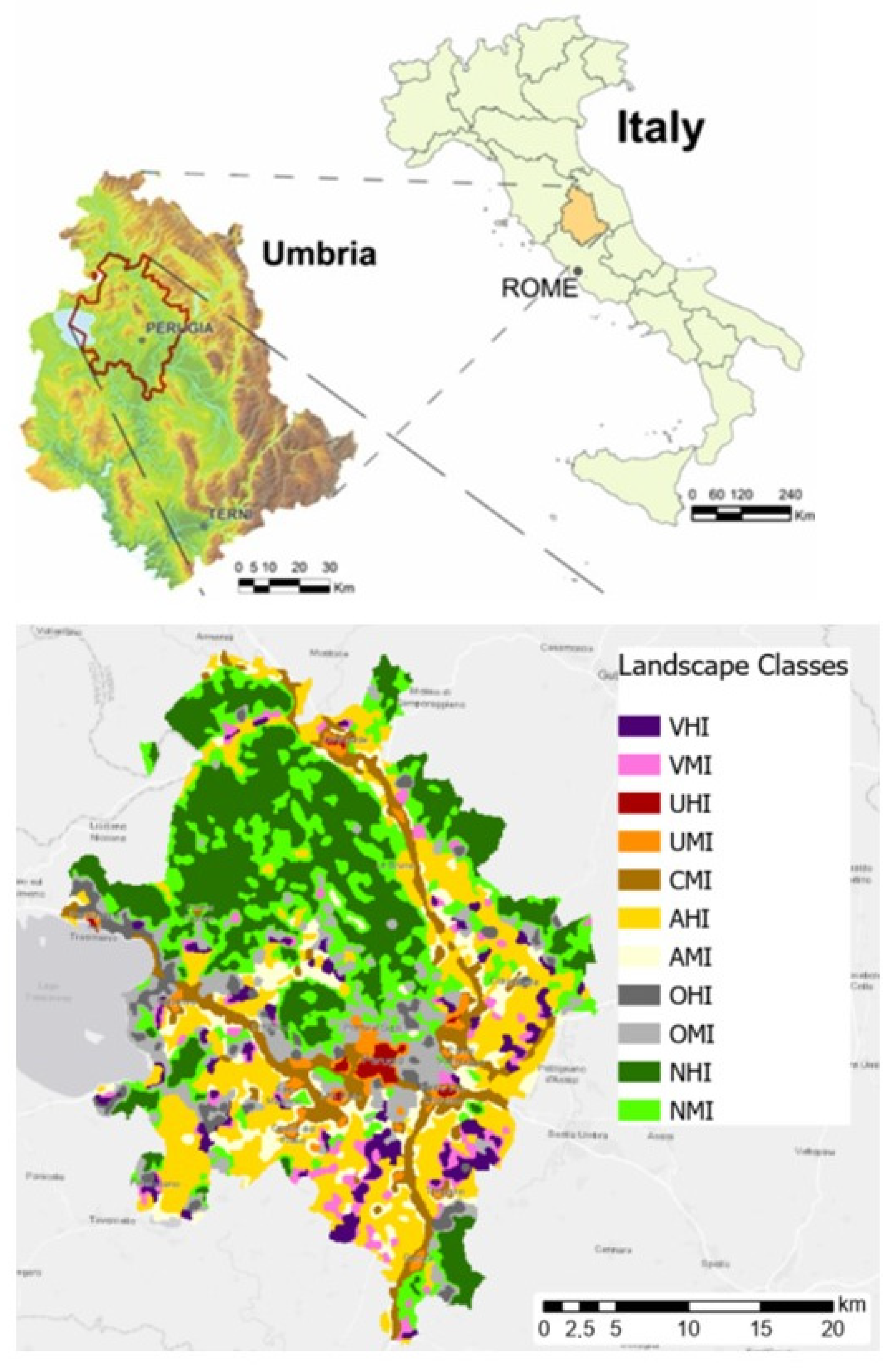
Two main steps were performed to meet the stated objectives: (1) SUSAM development and application considering different and verisimilar scenarios, (2) sensitivity analysis to test the sensitiveness to variations of judgements and the resistance to the variation of model’s indicators.

2.1. Study Area

The model was developed and tested in a 1007 km2 wide study area located in the Umbria region, Italy (43.077837° N, 12.420829° E). On average, the area is 332 m.a.s.l., has a transitional Mediterranean climate (sub-coastal in the western part and sub-continental in the eastern part, according to the Koppen classification), with hot, sunny summers and relatively cold winters. It includes the city of Perugia and its surroundings, covering seven different municipalities: Perugia, Magione, Passignano sul Trasimeno, Corciano, Umbertide, Torgiano, and Deruta (Figure 1). This area encompasses an urban and productive landscape of high territorial complexity that, in recent decades, has been characterised by high rates of urbanisation and related rural transformations. Land use patterns in the area are typical of central Italy, consisting of 58% agricultural land, 28% forested and semi-natural land, 8% built-up land, and less than 6% wetland and water bodies (personal elaboration from CORINE land-use and land-cover data [44]). The area is characterised by various landscape types, including natural areas as well as the arable, vineyard, and olive yard-dominated landscapes. A large proportion of the study area is characterised by various mixed transitional landscapes [5]. In such heterogeneous areas, landscape planning proves to be highly challenging, as it involves addressing conflicting needs of the human populations living and working in the area (e.g., nature conservation, economic development, agricultural production, housing, etc.).
Eleven landscape classes (Table 1) were identified in a previous study based on unsupervised classification of different LULC density features [5,45]. The methodology was aimed at detecting the landscape typologies along a gradient generated by a sliding level of anthropogenic influence on LULC. In this vein, the landscape classes can be considered homogeneous in LULC composition and can be ordered according to landscape sequences [46]. Their interpretation is highly informative, as it highlights different characteristics of the landscape [47]. For this reason, they were used as known reference areas for a better understanding of the variations of the SUSAM outputs.

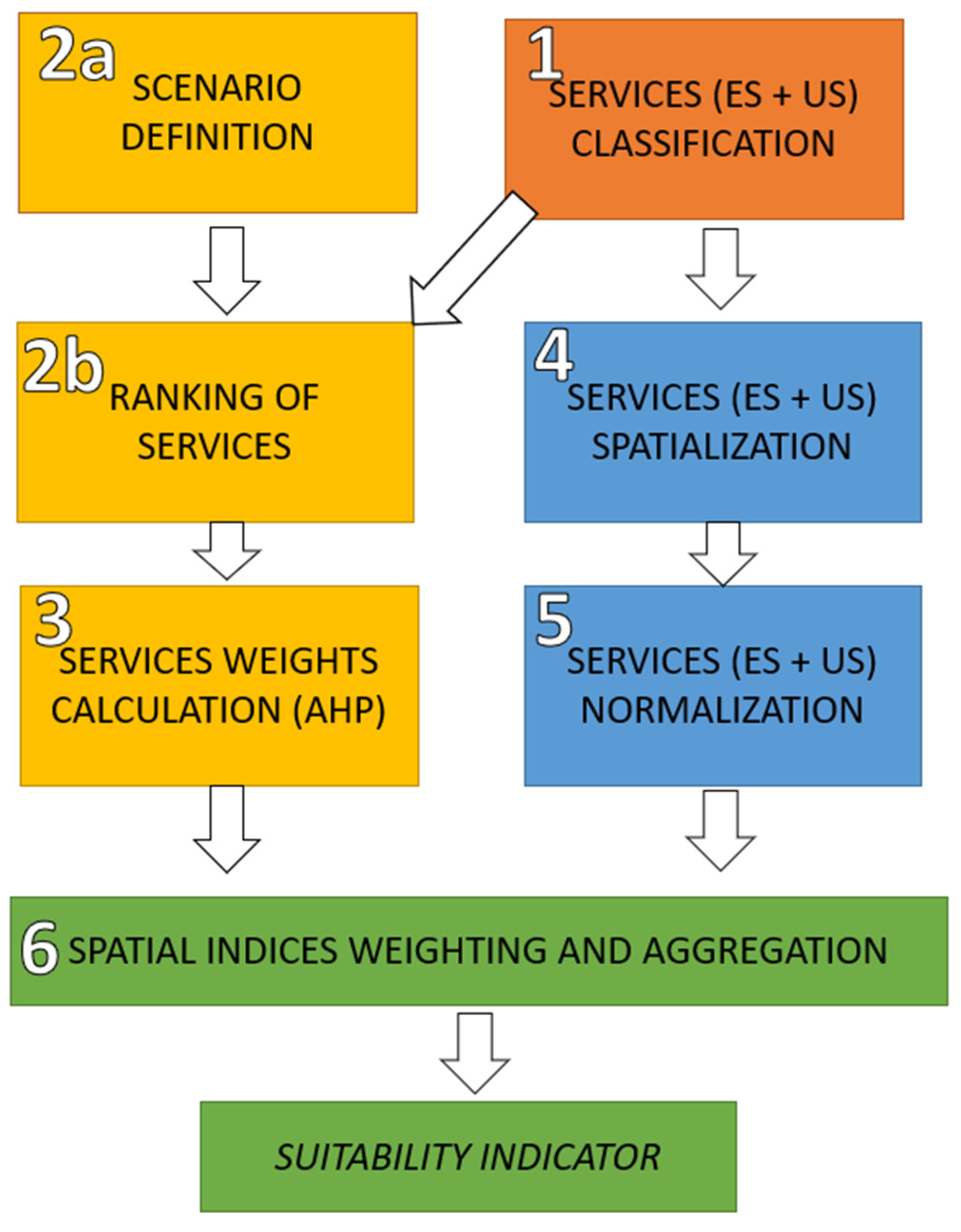
2.2. Model Development and Application

Comparably to its ancestor LISAM [13], the suitability spatial assessment model (SUSAM), developed in this study, is based on S-MCDA [14]. S-MCDA is a group of widely used techniques combining geographic information systems (GIS) and multicriteria decision aiding (MCDA). These techniques allow integrating spatial indicators (map criteria), preferences, and related uncertainties (value judgments) expressed by decision makers or stakeholders. The aim is to obtain information for decision making in an iterative, transparent, and consistent manner [48,49]. The analytic hierarchy process (AHP) [50,51] is a widely used approach within S-MCDA [52,53,54,55]. It is based on breaking down the decision-making model into a hierarchical tree. The main goal (in this case the “landscape suitability”) is at the top, and criteria (groups of services) and sub-criteria (services) are in the descending order within the hierarchy. According to a hierarchical scheme, the structure of SUSAM, derived from LISAM, allows the formulation of comparative judgments of criteria and sub-criteria. The judgements are expressed with iterative pairwise comparisons (PCs) between criteria or sub-criteria, within a reciprocal matrix (the pairwise comparison matrix—PCM) in which evaluations of the different factors are entered using the judgments from the decision makers). PCM is a method developed within the AHP and widely applied in similar studies [13,15,54]. Scaled indicators of services are progressively aggregated through weighted linear combinations to obtain the final suitability spatial assessment, using the weights of each service or group of services calculated at each hierarchical level.
Since the spatialization of suitability is aimed at defining areas providing services with different characteristics, in SUSAM, relevant scenarios were designed to apply and test the model. Each scenario is designed to represent the interests of a defined stakeholder group or the focus of a different decision. In each scenario, the relevance of a group of services with common characteristics is maximized to identify the areas with high intensity and density of the most relevant services.
SUSAM was developed in seven steps (Figure 2): (1) definition of a hierarchical classification including ES and US; (2a) definition of verisimilar scenarios and (2b) service selection and ranking; (3) attribution of relative weight to each service based on AHP. Then, steps dedicated to the spatialization of services in the area were performed: (4) spatial modelling of SBA and (5) normalization of services ranges into the study area. Finally, the final suitability index was obtained from the last step (6) oriented to weighting and aggregation of the spatial indices. Processes oriented to spatial analysis (Figure 2, in blue) and service ranking (Figure 2, in yellow) can be carried on parallelly, as they are independent of each other. In SUSAM, AHP is applied unusually, as steps 2 and 3 are typically developed in reverse order. This reversion, in this application, is necessary because, in the design of the scenarios, the service ranking (i.e., their order) is defined, while their relative importance (i.e., the difference between their importance) can only be estimated.

2.2.1. Definition of the Services’ Classification

In this research, LIAM 2.0 classification of services [12] was improved to be more effective for spatial applications supporting policy making. The supplementary material includes the list of services, the correspondent spatial indicators’ details, and the service codes (Table S1). LIAM 2.0 classification [8] was based on the Common International Classification of Ecosystem Services classification and is structured using three hierarchical levels: sections, divisions, and classes. LIAM 2.0 classification includes 53 final services, which can potentially support different and identifiable human activities, such as farming, commercial activity, housing, etc. A closer observation to the designed classification shows that services demand is restricted to three of the four demand typologies [56]: risk reduction, consumption, and direct use. This choice determines that the SBA gives benefits only to the use region located in the study area or nearby, since they are usually contiguous or relatively close, excluding from the study services having spatial relations at a broader scale. This choice helps the local policy makers’ focus on the services benefiting the areas they can actually manage.

2.2.2. Scenarios Definition and Ranking of Services

Different scenarios were designed and analysed for applying SUSAM. As introduced earlier, we considered scenarios derived from highly debated perspectives in the scientific literature: the economic activities and the need for infrastructures. Considering the different groups of economic stakeholders in a given area as a perspective to analyse the contrasting landscape economic activities’ needs, three scenarios were identified focusing on groups of services needed for agricultural activity, housing, and commerce and industry (Table 2). Regarding the perspective of the need for infrastructures, two scenarios were identified: the first focuses on the identification of areas where infrastructures are needed for reaching the services’ benefiting areas, while the second focuses on the identification of areas where the services can be benefited without infrastructures (these services cannot be replaced by those provided elsewhere) (Table 2). All the scenarios are linked to common situations occurring in the planning and management of multifunctional landscapes where decisions about land use–land cover changes to meet the needs expressed by the different stakeholder groups are often requested. Based on relevant previous works and empirical knowledge, services in the classification (Table S1) were divided into two groups for each scenario (Table 2): important and non-important services. As a reference for the analysis of scenarios, we calculated a baseline result hypothesizing that the respondent would give the same importance to all the services. This baseline was used to perform the subsequent sensitivity analysis and show the model applicability for the suitability assessment.

2.2.3. Services’ Weights Calculation

After defining which of the services included in the classification can be considered relevant for each scenario, high relative importance was attributed to them through the PCMs. For each couple of services, two questions are asked to fill the PCM: which of the two services is more important and how much it is more important than the other service. The same comparison was made for each service section and division. A semantic scale, representing the ratio among them, as defined by [50,51], was used to compare couples of services. From the PCMs, absolute scales of relative values (importance) were obtained based on principal eigenvectors and, then, by normalizing them by dividing each value by the sum of all the values. For the studied scenarios, the relevant services were highlighted in the study area, giving them a score of 9 from Saaty’s scale. The relative importance of divisions and sections was calculated based on the proportion of the relevant services included in each group. Final services weights were calculated after filling the PCMs.

2.2.4. Services Spatialization

In this step, we broadly used spatial indicators of services included in LIAM 2.0 classification quantifying the service provided in their SBA [12]. Besides, the indicators of 17 services, mainly regulating or provisioning, were calculated ex novo to quantify the services included in the model, while other indicators from LISAM [13] were used for quantifying other services. For specific services or a group of services, additional spatial indicators were calculated to integrate those provided by LIAM 2.0. The methodologies used to define and calculate these indicators are described in Appendix A. The complete list of spatial indicators used in this research, complete with various additional information, is reported in the Supplementary Material (Table S1).

2.2.5. Service Indicators’ Normalization

In the AHP, indicators are usually scaled between 0 and 1 to be comparable and integrable with their relative weights possible. To this purpose, service indicators can be scaled using different methodologies based on the purpose of the study. In this work, to calculate suitability, the model was run using two linear scaling approaches: the supply-based scaling, according to which 0 was associated to the minimum value of the indicator, and 1 to the maximum value of the indicator in the study area; the demand-based scaling, according to which 0 was associated to the minimum level of the indicator required by the demand and 1 to the values of the indicator able to meet the demand completely. The former method was targeted at expressing the relative quantity of service supply. In this case, each indicator is scaled between its minimum value and maximum value in the study area. So, the resulting indicator has only a relative value clearly expressing the differences within the area in terms of supply and is not comparable with other study areas. Differently, with the latter method, indicators were scaled based on demand-driven minimum and maximum to obtain indices potentially comparable with other areas.
In the demand-based scaling approach, we considered that services demand is influenced by two main factors: population beliefs and preferences, which are variable across space and time [60], and biophysical characteristics of the landscape. Only this last variable was considered to identify minimum and maximum values of service demand. So, the potential service demand of each service needed to be assessed before performing the demand-based scaling. The demand was considered constant in some cases, while in others, it varied across space due to physical landscape features (such as slope, presence of specific land uses, etc.).
Depending on the type of service indicators used in the study (presence–absence indicators or intensity indicators, further differentiated in two sub-types each), we identified a different method for defining the potential demand (Table 3, Table S1).

2.2.6. Weighting and Aggregation of Spatial Indices

Service indicators, weighted by their percentage importance for the suitability, were used to calculate a spatial suitability index (SI) for each scenario defined in this study. To this aim, following the methodology used for the LISAM model [13], raster layers representing local service availability were progressively aggregated at the three hierarchical levels through multiple weighted linear combinations implemented in ArcGIS scripts using the graphical modeller.
Due to the unavailability of pertinent data and reliable indicators, some of the services were not mapped in this specific application and so were not included in the overall suitability index. Since the completeness of the resulting suitability index in each place depends on the weights of the spatialised services, the sum of these weights was used to express the proportion of “explained suitability”. This approach is similar to that used for the LISAM development [13]. Spatial statistics of each suitability index were calculated for the eleven landscape classes in the study area to interpret the results (Figure 1). This step was helpful to interpret better and compare the results of the model’s application in the various scenarios.

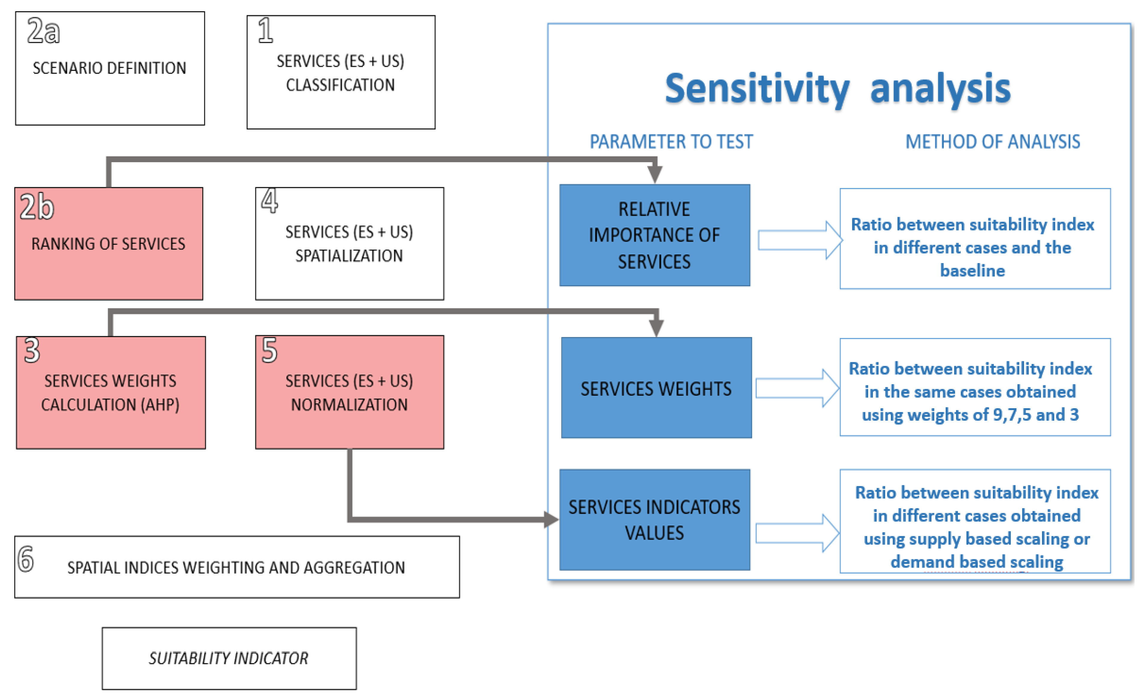
2.3. Sensitivity Analysis

A landscape suitability assessment model should be sensitive to variations of judgements, while it should be pretty resistant to the indicators’ variation. Thus, an extensive sensitivity analysis appeared very important to understand the level of responsivity of SUSAM to the variation of preferences about services and the variation of the indicators’ level. In this direction, we considered the three main factors mainly influencing results variability in a typical S-MCDA model [42]: (1) service indicators values, (2) relative importance of services, and (3) service weights. To test sensitivity for each scenario, we fixed the different parameters of the model, varying one of the variables (Figure 3). Couples of suitability index outputs were compared by calculating ratios per landscape class to understand better the entity and the localization of the effect of the varying parameter on the results.

2.3.1. Understand the Model’s Behaviour under Changing Service Values

The model was applied to the baseline case and the five scenarios under analysis using supply-based scaling and demand-based scaling. These applications were performed to test how much SUSAM’s results change due to the method used to scale service indicators. Then, average suitability values in each landscape class were calculated. The ratios between SI calculated using supply-based scaling and demand-based scaling were calculated for each case to better compare the service value’s effect on the results.

2.3.2. Understand the Model’s Behaviour under Changing Services Ranking

To understand the model’s sensitivity to the change in the relative importance of criteria in terms of spatial pattern and suitability values, SUSAM was applied to the baseline of the five scenarios under analysis, both applying supply-based scaling and demand-based scaling. Then, average suitability values in each landscape class (Figure 1, Table 1) were calculated. The ratios between SI calculated for each scenario and the baseline were calculated.

2.3.3. Understand the Model’s Behaviour under Changing Service Weights

The model’s sensitivity to the changes in weights of criteria was tested to understand how this factor affects the results in terms of services’ relative weight or services’ ranking. This step was performed on the three economic activities’ scenarios (FARM, HOUS, and COMM). In each scenario, the effect of relative weights of 3, 5, 7, and 9 from the Saaty’s scale, applied to the services defined as “important”, was measured, and the results obtained were compared. This comparison was performed by calculating the ratios between sequential weights (9/7, 7/5, 5/3, and 3/baseline) for each landscape class. These weights were chosen because PCMs are commonly filled based on five linguistic indicators that correspond to the main numerical weights (1, 3, 5, 7, and 9), while the intermediate ones (2, 3, 6, and 8) are rarely used [52].

3. Results and Discussion

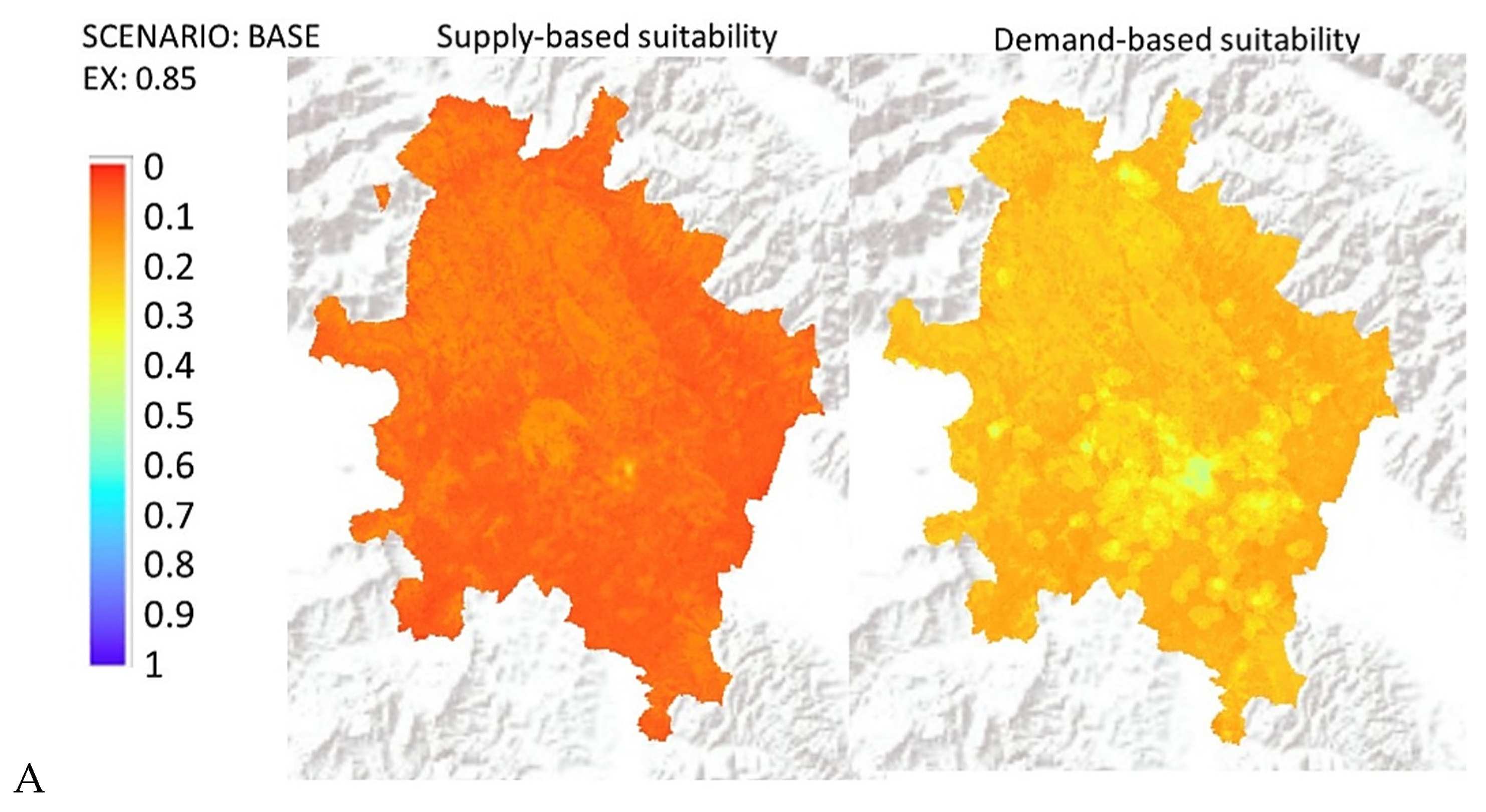
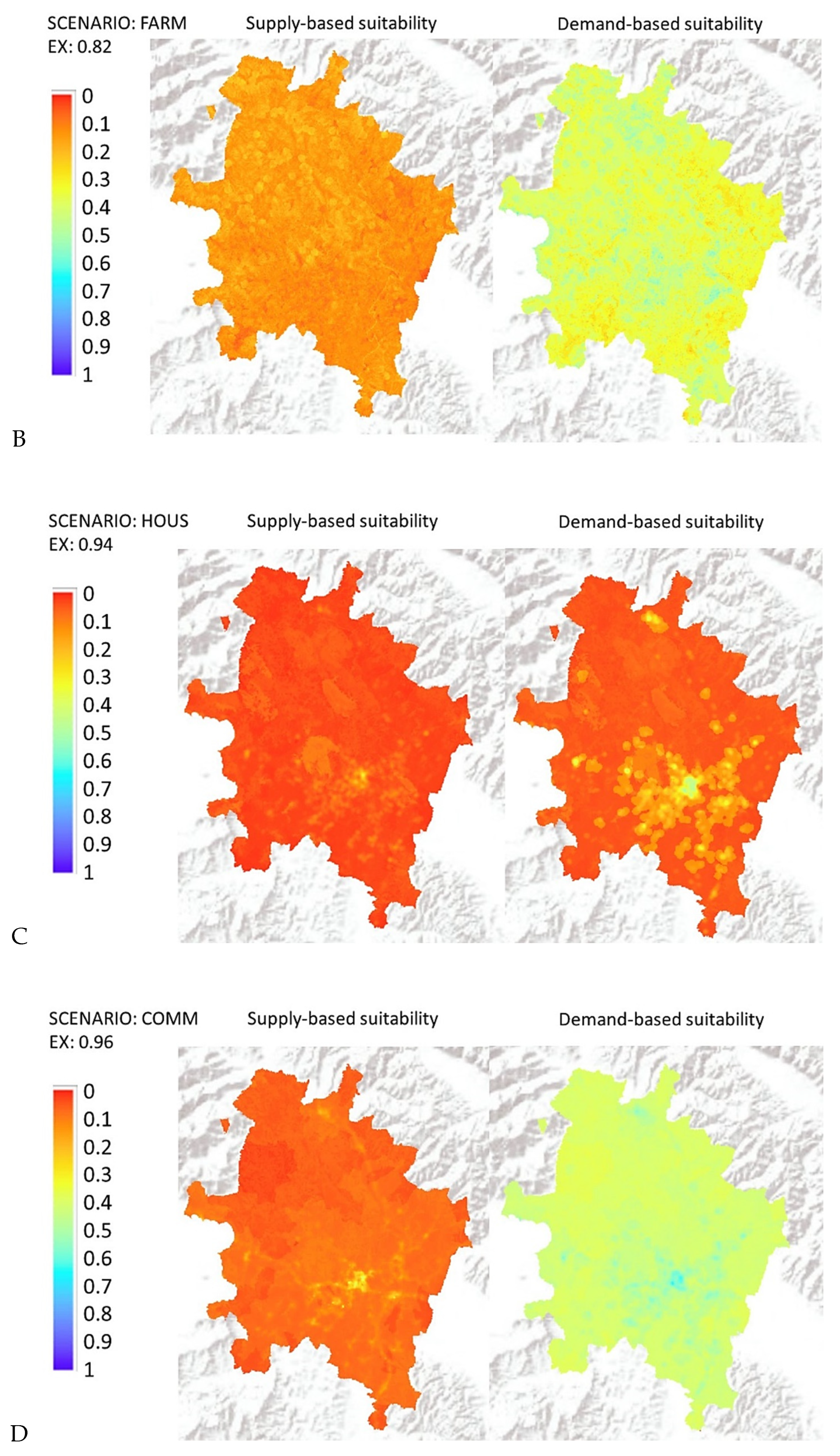
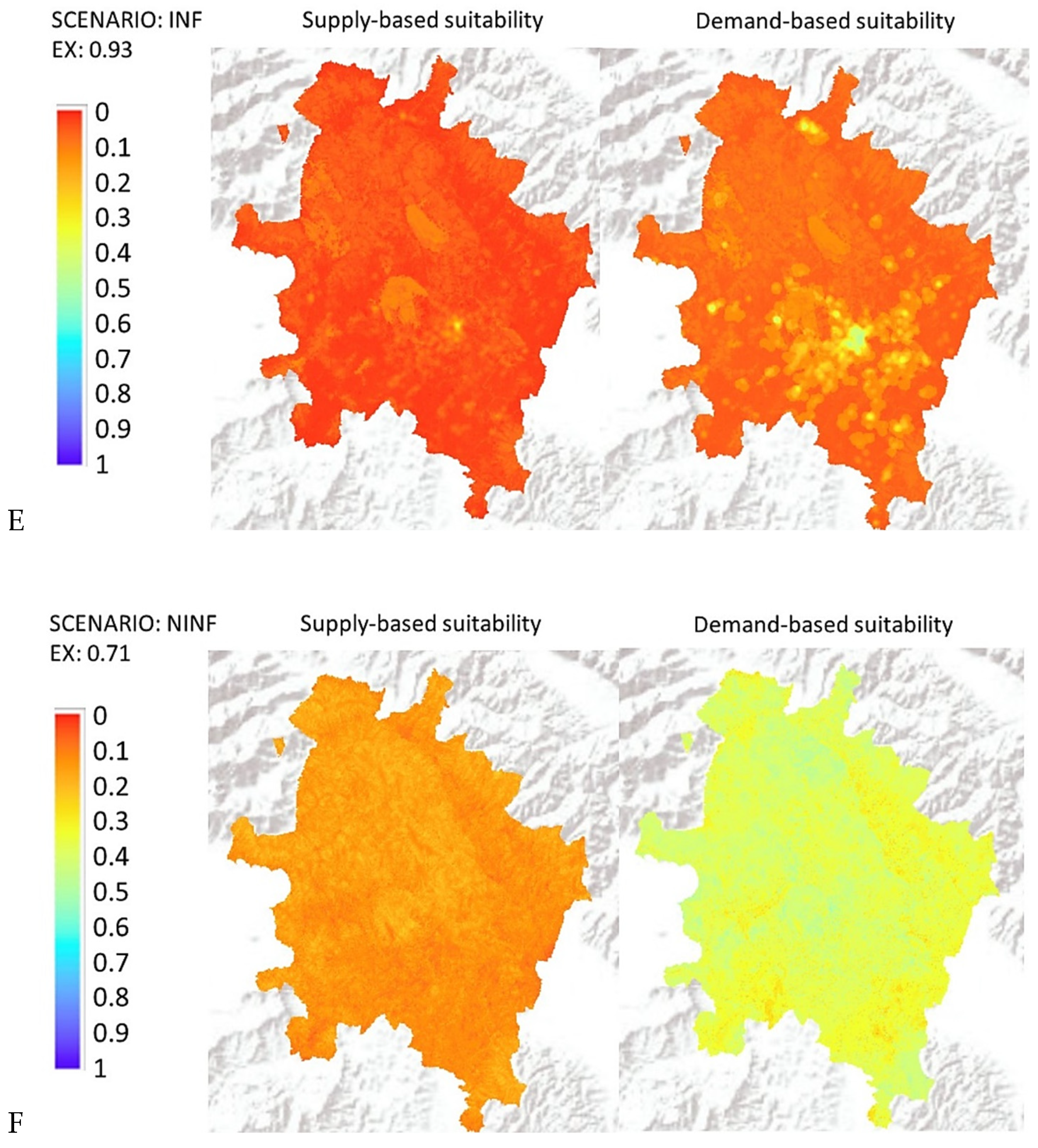
3.1. Landscape Suitability Assessment

The model application results for the suitability assessment are shown in Figure 4 and Figure 5 (baseline and the five scenarios). Supply-based suitability identifies the landscape areas where there is a relatively higher presence of services. Demand-based suitability shows, in percentage, how the different locations of the landscape fulfil the potential demand of services. The application of the model in the baseline scenario resulted in non-uniform levels of suitability across space. These results are driven by the higher presence of services in the more urbanized areas, representing the benefiting areas of many of the services included in the classification. In the first case, when supply-based indicators are used, suitability is comparably higher in natural landscapes, where many cultural services are provided in relatively high quantities. When the demand-based scaling is used to calculate the results, suitability is generally higher than in the first case in the whole study area. In contrast, the highest levels are clearly shown in the more urbanized landscapes, where urban services are provided. In both cases, landscapes dominated by agricultural features such as olive yards (OMI and OHI), arable lands (AHI and AMI), or vineyards (VHI and VMI) are suffering from a lack of suitability due to the low presence of different categories of services, mainly cultural.
The explained suitability, representing the percentage of suitability for which indicators are available, is generally high, ranging from 71% to 96% in the cases under analysis, since we spatialized 49 on 53 services included in the classification.
The application of SUSAM in the selected scenarios shows that the highest value of suitability usually characterizes the urbanized landscapes (UHI and UMI). Results from the supply-based scaling show that values of suitability for agricultural activities (FARM) are higher in the agri-natural areas. In contrast, the demand-based suitability is higher in urban and peri-urban areas, showing high possibilities for the whole area to perform urban agriculture. In fact, the land and environmental conditions are also generally good in the city centre, while materials are generally well available. The housing scenario (HOUSE) shows, as expected, its highest values in the UHI landscape, with both types of scaling. UMI and CMI landscapes also show relatively high levels of suitability for housing if compared to other landscapes, meaning that the urban component is highly benefiting this group of activities. Inversely, suitability to housing is considerably low in other landscapes.
The supply-based and demand-based values of suitability for the commercial activity scenario (COMM) are also increased by the landscape’s urban component, particularly by the main roads and fast internet connection. The highest levels of this kind of suitability appear in the UHI landscape, where the demand-based SI reaches 0.66, which is the maximum value reached by the indicator in the whole study area. The explained suitability is high in each case, ranging between 0.81 and 0.96.
When SUSAM is applied to produce maps for identifying the areas that need infrastructures (INF), results show that the more urbanized areas (UHI, UMI, and CMI) typically need roads and transport infrastructures. This tendency appears more evident when demand-based scaling is applied. Similarly, the suitability of natural landscapes (NHI and NMI) to roads and transport infrastructures is also high, since they deliver services that can only be benefited in loco. On the other side, when the areas with no need for infrastructures are highlighted (NINF), the suitability shows higher values in all the landscapes. However, the percentage of explained suitability is relatively lower (0.73). In this case, agricultural and natural landscapes produce more directly delivered services to the use regions than urban landscapes (UHI, UMI, and CMI).
These results indicate how the scaling method represents a crucial factor determining noticeable quantitative differences in landscape suitability. This evidence is due to their different mathematical meaning: on the supply-based scaling, the result is relative, and for each indicator, there are always a value of 0 and a value of 1 in the study area, while when demand-based scaling is applied, indicators represent the percentage of potential demand that is satisfied. Thus, the two scaling methods give a different meaning to the final suitability indicator: when supply-based scaling is applied, indicators effectively identify the areas with service scarcity, while when demand-based scaling is applied, SUSAM gives informative results about the satisfaction of potential demand. Since many essential services are equally provided across the whole study area, the demand-based scaling results in a lower level of differentiation between landscape areas, but the resulting suitability is also potentially comparable with the index from other study areas, scaled with the same method. On the contrary, supply-based scaling is more effective in highlighting differences within the area, guiding policy makers more effectively towards comparing the different locations within their administrative areas.
The application of SUSAM for identifying the areas where services needing accessibility are concentrated (INF) highlights the crucial role of accessibility for these areas to benefit the supplied services. In fact, accessibility, defined as the potential opportunities that can be reached from a given place by paying a specific generalized and space/time-based cost [61], is a vast and complex concept that needs deep understanding to be adequately quantified also considering its spatial nature. As suggested by [13], accessibility can be used as a proxy for assessing service supply, but its application can limit the use of indicators able to quantify the service supplied. So, further investigation is needed to integrate service quantification with their accessibility assessment.

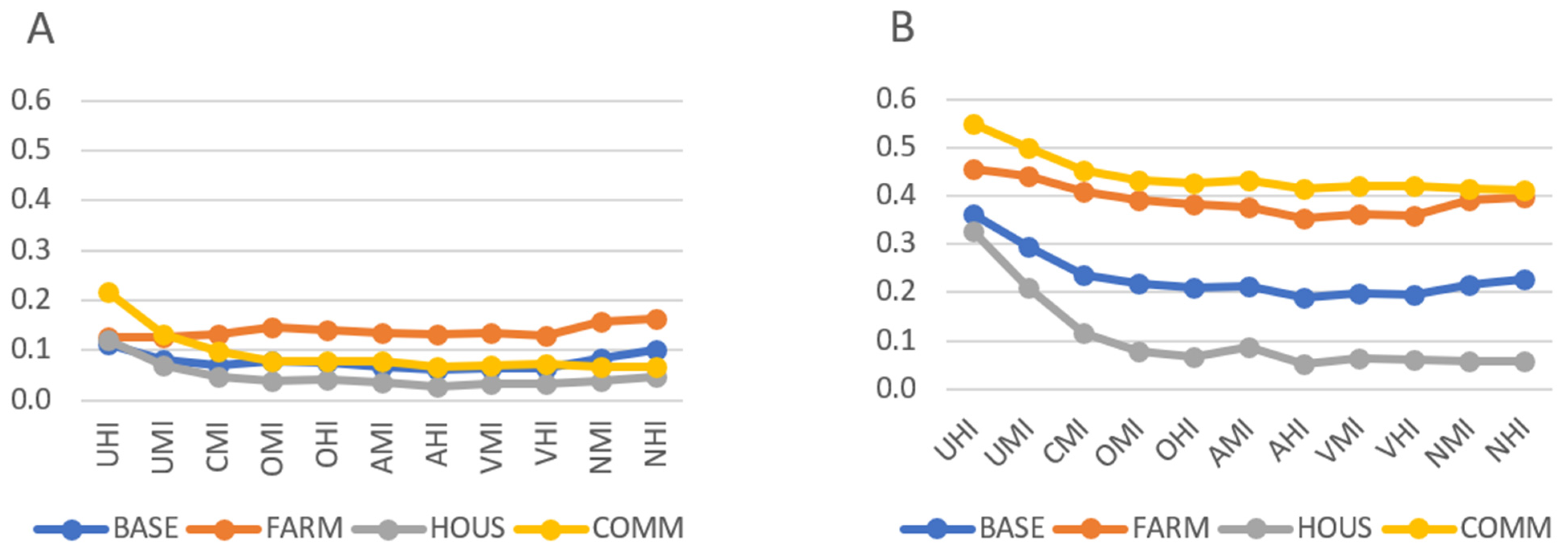
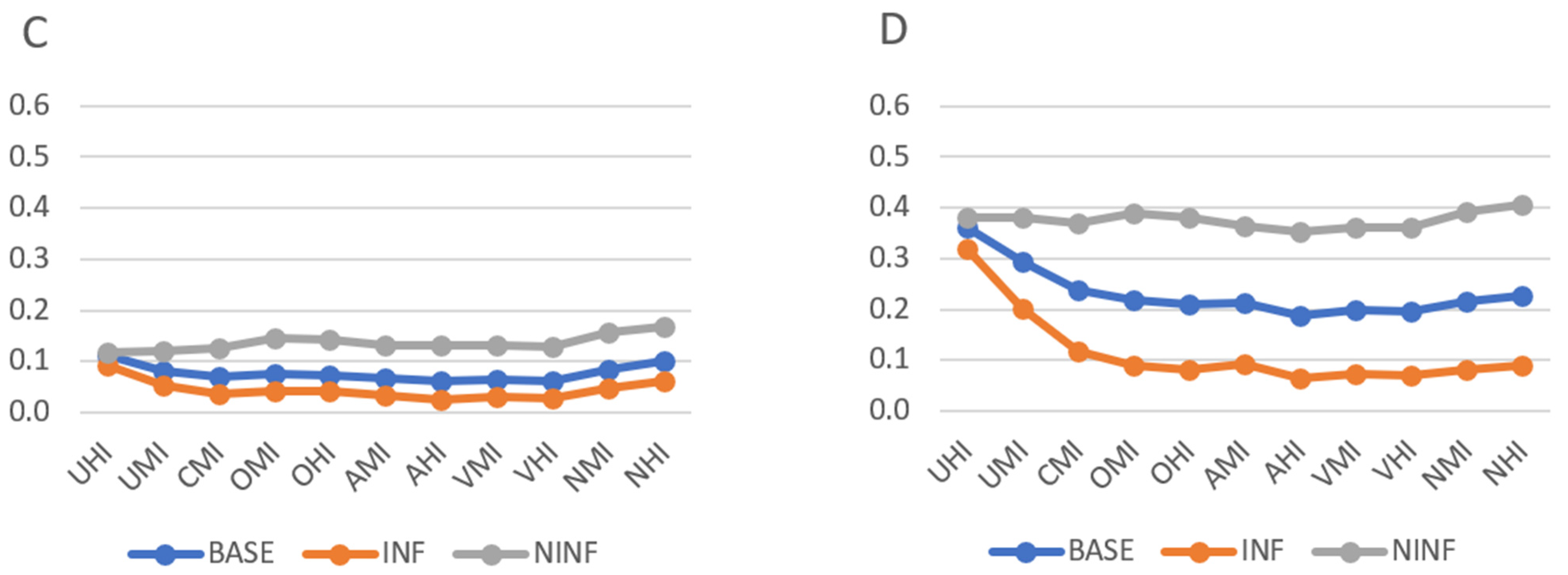
3.2. Sensitivity Analysis

3.2.1. Model’s Behaviour under Changing Service Values

Ratios between suitability calculated applying the supply-based approach and the demand-based approach are reported in Figure 6 for the different scenarios under investigation. Results show that the values are lower than 1. Moreover, the graphs show few relevant differences between the results in different landscape classes, while there are some evident differences in ratios between the different scenarios.
In the analysed cases, demand-based suitability is higher than supply-based suitability, meaning that the area has an excellent capacity to fulfil human needs even in landscapes with a relatively low quantity of service supplied. Demand-based suitability is generally higher and flatter than supply-based suitability. A reason for that is that some services typically satisfy all the potential demand in the area, despite varying the supplied quantity. For example, soil fertility varies across the area, generating variability in supply-based suitability. However, the soil fertility is generally rated as “very good” across the whole area, flattening the differences between the different landscapes. This consideration is also valid for other services, such as water provision for drinking purposes. This evidence is also supported by the fact that in those landscape classes where the supply–demand ratio shows high values, suitability is also high. The contrary happens in the areas with low liveability values, where the differences between supply-based and demand-based indicators are more evident. For example, in COMM, a scenario mainly benefiting from services produced and delivered in urban areas, the supply-based suitability of urbanized landscapes is high, and the supply-based and demand-based values of the index are more similar. In the scenarios INF and HOUS, landscapes NHI, NMI, OMI, and OHI show the highest ratios, meaning that in these cases, supply-based and demand-based suitability are pretty similar. So, landscape type is relatively suitable to the purpose identified because it offers a high density of maximized services.

3.2.2. Model’s Behaviour under Changing Services Ranking

The analysis of ratios between specific scenarios and the baseline support the understanding of the suitability indicator’s sensitivity to the variation of the relative importance of services (Figure 7).
Results from this analysis show that the relative importance of services strongly influences the final SI. When this factor varies, the suitability is reduced to 75% or increased up to 220% if compared with the baseline. When the importance of services needing accessibility is maximized (in INF and HOUS scenarios), suitability tends to decrease compared to the baseline. On the contrary, when the importance of services that do not require accessibility is maximized, suitability tends to increase compared to the baseline. This happens in NINF and FARM. These trends suggest that each landscape type offers high quantities of the services maximized in NINF and low quantities of the services maximized in INF and FARM. In the cases discussed above, suitability shows similar trends with supply-based scaling and demand-based scaling. However, in the COMM scenario, where many essential services are required, suitability is higher than the baseline in the demand-based suitability. Differently, it shows a different trend in supply-based suitability.

3.2.3. Model’s Behaviour under Changing Service Weights

Results reported in Figure 8 show the suitability values in the economic activities’ scenarios under changing service weights in the different landscape classes.
These results show clearly that the effect of the weights’ increase with inverse proportionality to the weight increment both in supply-based and demand-based suitability index. This evidence means that weights have a slight influence on suitability, while the services’ ranking influences the results strongly, as the diversity of trends shown by the different cases shows. Moreover, since the graphs show an equal shape of the curves in Figure 7 (scenarios calculated with a relative weight of 9/indifference case), it is possible to conclude that the relation between the weights’ increase and the suitability increase is monotonic in each scenario analysed.
In general, the sensitivity analysis showed that the services’ ranking strongly influences results. On the one hand, it means that the model is very sensitive to stakeholders’ preferences, and it can be used to measure suitability, differentiating results based on such preferences. On the other hand, these results indicate that the model is more sensitive to the relative importance of criteria than their relative weight. This evidence suggests that when PCMs are filled, and two questions are asked for each pair of services compared (“which service is more important between these two?” and “how much this service is more important than the other one?”), the answer to the first question is much more important than that to the second one. Consequently, more accuracy is required for the definition of the service ranking than for the service weight. In this view, since PCMs’ completion is a really demanding technique to calculate service ranking, as the number of pairwise comparisons can become overwhelming [62], different techniques, such as ranking or scale rating [63], could also be used for defining service order to simplify the definition of relative importance at the expenses of the service weight accuracy. In this direction, further investigation may be necessary.

4. Conclusions

This research developed an S-MCDA model, called SUSAM, for the spatial quantification of landscape suitability, intended as the landscape ability to provide services with common features as preferred by specific groups of stakeholders. This application showed that SUSAM could effectively produce a spatial index of suitability, highlighting areas with different provision degrees of a defined group of services, producing informative indicators for landscape policy makers.
The sensitivity analysis applied on SUSAM showed that the relative importance of services (services ranking) heavily influences the results, demonstrating that the method is highly sensitive to the change in scenarios, and therefore very helpful for supporting landscape analysis for policy making. The service relative weights only secondarily influence the results, especially if the weights used in the comparison are lower than seven. This evidence suggests an uncertainty reduction in the suitability assessment, since the weight can be more complex to define than the ranking of services. The service indicators’ values are highly influential on the SUSAM results, meaning that the choice of the indicators and the methodology for their normalization should be carefully evaluated for an effective SUSAM application.

Supplementary Materials

The following are available online at www.mdpi.com/article/10.3390/app11178232/s1, Table S1: SUSAM service list in MS Excel format, including the correspondent spatial indicators’ details, and the service codes.

Author Contributions

Conceptualization, S.A., M.V.; methodology S.A., M.V.; investigation, S.A.; data curation, S.A.; writing—original draft preparation, S.A., M.V.; writing—review and editing, S.A., M.V.; visualization, S.A.; supervision, M.V. All authors have read and agreed to the published version of the manuscript.

Funding

This research was developed within the framework of the Towards Rural Synergies and Trade-offs between Economic Development and Ecosystem Services (TRUSTEE) project funded by the RURAGRI ERA-NET Consortium (project number 235175), which includes the Italian Ministry of Agricultural, Food and Forestry Policies.

Institutional Review Board Statement

Not applicable.

Informed Consent Statement

Not applicable.

Data Availability Statement

Data are available, upon any reasonable request, from the authors.

Acknowledgments

The authors wish to thank Catharina J. E. Schulp of the Environmental Geography Group, Institute for Environmental Studies, Vrije Universiteit Amsterdam, for her valuable collaboration during all the research steps.

Conflicts of Interest

The authors declare no conflict of interest.

Appendix A

Additional spatial indicators developed in this research for quantifying specific services or group of services (the indicator codes reported in Table S1 are indicated in parenthesis):
  • Habitat suitability for the most common edible species. It quantifies the provisioning of nutrition goods “wild plants, algae and their outputs” (112wildpl) as suggested by [64]. The indicator was calculated as follows:
    Data collection: Data from Global Biodiversity Information Facility (GBIF) database were collected for each edible plant and fungi species localized in the study area. Information about edible species was retrieved from actaplantarum.org (accessed on 15 April 2020). A geobotanic map was used as a database of the land use of the area;
    Calculation: The potential habitats of each different species were listed and, then, identified on the geobotanic map. The elevation at which each species typically live was also considered to define each species’ potential habitat better. Then, a buffer of 5 km around the potential service benefiting area was built [55] to select the landscape areas where the service can benefit the residents. The potential habitat areas of each edible species were selected between the many land uses included in the buffer. The service indicator was calculated as the sum of the species potentially present in each point of the study area. As nine edible species were assessed, the indicator value varies between 0 and 9.
  • Building density: It is used as an indicator for provisioning of nutrition goods, namely groundwater and surface water availability for drinking purposes (115grdrin, 116 surdrin) and energy from fossil fuels (134netener). This indicator can be considered a meaningful proxy of the quantity of these services, as, in Italy, they are associated by law with the construction of new buildings. The radius used for the Kernel Density Estimation is 200 m, which is the distance from the electricity cabin at which a typical local electricity service asks for a supplementary payment. It is calculated as follows:
    Data collection: a municipal database was used to extract buildings, their covered areas, and their number of floors;
    Calculation: Kernel density estimation (KDE) of the total floor area of buildings, obtained by multiplying the number of floors of a building by the building dimension.
  • Easiness of wells digging: It is used as an indicator of the service: provisioning of groundwater for the non-drinking purpose (intended as material for different production uses) (122grnodrin). The indicator was calculated as follows:
    Data collection: A database from local public authorities reporting the wells registered across the territory was collected. This database also includes the wells’ depth;
    Calculation: inverse distance weighting was applied to the difference between the maximum depth of a well (conventionally defined as 50 m) and the actual well depth.
  • Average water yield from rivers and water reservoirs was calculated to quantify the provisioning of surface water for non-drinking purposes (123surnodrin). The service was spatialized based on the following empirical observations: (1) a total amount of 2% of the average river flow can be used for industrial and agricultural uses; (2) about 40% of the total volume of reservoirs is available yearly. The indicator was calculated as follows:
    Data collection: a database of the water reservoirs, indicating the water volume capacity, and a database of the rivers and streams, indicating the average flow rate, were collected from local public authorities;
    Calculation: River flow rates and water reservoir volumes were multiplied by the percentages of availability observed empirically, resulting in the calculation of the average daily water availability. This value was distributed on a 50 m buffer area around each watercourse or reservoir.
  • Coppices: It has been used to estimate the provision of plant-based resources for energy (131planres). The indicator was calculated as follows:
    Data collection: The forest map of Umbria was used as a dataset for the estimation of this indicator. It categorizes the forests with many attributes, such as accessibility of each forested land, which were assessed in the forest map, mainly based on slope;
    Calculation: the intensity of the service delivery was based on the levels of forest accessibility defined by the map: 1 = not sufficient, 2 = low, 3 = good.
  • Energy plants powered by livestock manure. It was used to map the provision of animal-based resources for energy (132animres). The indicator was calculated as follows:
    Data collection: a municipal database of energy plants powered by livestock manure, including each plant’s maximum power, was used;
    Calculation: Biomass plants powered by manure were spatialized based on coordinates reported in the municipal databases and integrated with local knowledge. Then, the maximum power produced by each plant was used to define service intensity. The service was spatialized by a KDE application (radius = 50 m), since the energy produced can be transported from the plant at increasing costs with increasing distances.
  • Cumulated avoided runoff due to land cover. It expresses the buffering and attenuation of mass flows in river basins and flood protection by natural subsystems (211ecoflood). This service, delivered downstream by the water retention property of soils, is a regulating service of natural physical phenomena:
    Data collection: A database of the rivers and streams from the local authorities was used to localize water streams. The geobotanic map was used for the LULC definition, while the EU-DEM [65] was used to define topographic variables, such as slope;
    Calculation: The soil conservation service curve number (SCS-CN) equation was used for calculating runoff [66,67] both in the actual situation and in a theoretical worst case, where all the study area is covered by built surface. The areas covered by rivers and water streams were excluded from the results. Based on [68], soil moisture was set as 20% of the potential maximum soil retention (S) in both cases, and the rain event considered was the highest one-day precipitation amount of the last ten years (100 mm) [69]. The cumulated upstream runoff reduction was calculated as the cumulated difference between the worst-case runoff and the actual runoff in each cell.
  • Percentage of avoided runoff by artificial reservoirs at sub-basin scale. It expresses the buffering and attenuation of mass flows in river basins and flood protection by human subsystems, a regulating service of natural physical phenomena (212urflood). The service was calculated as follows:
    Data collection: a climate database of rain was used to analyse precipitation amounts, while sub-basins were defined based on EU-DEM dataset;
    Calculation: Total water runoff per each sub-basin was calculated by SCS-CN equation [66,67], setting the soil moisture as 20% of the potential maximum soil retention (S) [68], while the rain event considered in the model is the highest one-day precipitation amount of the last ten years (100 mm) [69]. Then, the total volume of reservoirs in each sub-basin was calculated. At the sub-basin level, the indicator intensity was calculated as 30% of the ratio between the total volume of the reservoirs and the total water runoff.
  • Amount of avoided erosion by agri-natural surfaces and urban surfaces. These indicators were used, respectively, to spatialize services for the regulation of natural physical phenomena, namely the mass stabilization and control of erosion rates by natural (213ecoeros) and human (214urberos) subsystems:
    Data collection: geobotanic map and EU-DEM were used as input databases;
    Calculation: The amount of avoided erosion was calculated as the difference of eroded soil in the actual situation and in a theoretical worse case, where all the surface was supposed covered by bare soil. For this purpose, the revised universal soil loss equation (RUSLE) was applied [70]. While R is considered constant, the K factor (soil erodibility) from [71] was used in agricultural and natural areas. The K factor in urban areas was roughly estimated using focal mean, with radius = 500 m. The length and slope (LS) factor was retrieved from [72], while C was calculated associating the RUSLE C factor tables to land covers indicated in the geobotanic map. Since the anti-erosion effect is delivered locally, the avoided erosion was clipped into urban areas for estimating service 214, while it was clipped into the other lands’ uses for estimating the quantity of the service 213 delivered.
  • Average pest predation rate. It quantifies the pest and disease control by natural subsystem, which is a regulating service for maintaining physical, chemical, and biological conditions (231ecopestcont). For the indicator calculation, we adapted the methodology suggested by [73]:
    Data collection: The geobotanic map was used for the identification of land use and land covers. A map of the linear features was autonomously designed by photo interpretation;
    Calculation: Habitats of pest predators were identified on the geobotanic map and the linear features map. Then, the percentage of LULC covered by the predators’ habitat in a radius of 2 km was calculated by focal mean. Then, the predation rate was calculated by the following equation [73]:
    19.65 + (0.309 × A)
    where A is the average habitat size of a given natural predator.
  • Land quality indicator. It expresses a service within the division of “maintenance of physical, chemical, and biological conditions”, namely the weather decomposition and fixing processes (234pedogen). For the calculation of this indicator, we adapted the methodology suggested by [74]:
    Data collection: www.isric.org/explore/soilgrids (Accessed on 6 May 2020) database at 250 m resolution was used for mapping fertility factors;
    Calculation: To calculate the land quality indicator, scores suggested in the paper were attributed to five fertility factors (organic C content, clay + silt, pH, cation exchange capacity, and soil depth). The factors were reclassified as “poor” (1), “medium” (2), “good” (3), and “excellent” (4) and, then, summed, producing an indicator with a minimum value of 5 and a maximum value of 17. Zero was associated with the urban areas.
  • Areas contributing to water flows in forested or wooded areas. This indicator was used to spatially quantify the maintenance of chemical conditions of freshwater by natural subsystems (235ecowatqual), which is a regulating service for the maintenance of physical, chemical, and biological conditions:
    Data collection: geobotanic map and EU-DEM were used as input databases;
    Calculation: Flow accumulation was calculated for the whole study area to calculate this indicator. Then, only the forested cells—the service provisioning area of this service—were selected.
  • Buffer from depurators. It was calculated to map the maintenance of chemical conditions of freshwater by human subsystems (236urwatqual), which is a regulating service for the maintenance of physical, chemical, and biological conditions. The indicators spatialize and quantify the ability of man-made systems to maintain clean water:
    Data collection: a database of local depurators was collected from public authorities;
    Calculation: A 500-metre buffer was considered adequate for mapping the SBA, since all the depurators are nearby the rivers. The intensity considered is represented by equivalent inhabitants.
  • Recreational potential of the agri-natural areas. It expresses the experiential and physical potential use of plants, animals, and land/seascapes in different environmental settings (313ecouse). It is a service related to the physical and intellectual interaction with the agri-natural environment [75]. The indicator was developed considering a previous research [76]:
    Data collection: geobotanic map was used as an input of the indicator;
    Calculation: Different scores of recreation potential ranging from 0 to 9 were attributed to the different land-uses in the study area to calculate this indicator. Then, the effect on surrounding areas was summed or subtracted from the base score. In detail: the baseline indicator was used when the cells were surrounded by arable land. When water, forests, or urban areas were within 1 km from a cell, their positive influence was considered. A KDE (radius = 1000 m) was applied to the streams and coasts and then scaled between 0 and 1 to calculate this influence. Then, the watershed effect was added to the baseline indicator. The effect of urban areas was added in the same way, while the effect of forests and woods was added by KDE addition, scaling the results between 0 and 2.

References

  1. MA (Millennium Ecosystem Assessment). Ecosystems and Human Well-Being: A Framework for Assessment; Island Press: Washington, DC, USA, 2003; ISBN 1559634022. [Google Scholar]
  2. Duraiappah, A.K. Ecosystem Services and Human Well-being: Do Global Findings Make Any Sense? Bioscience 2011, 61, 7–8. [Google Scholar] [CrossRef]
  3. Burkhard, B.; Kroll, F.; Nedkov, S.; Müller, F. Mapping ecosystem service supply, demand and budgets. Ecol. Indic. 2012, 21, 17–29. [Google Scholar] [CrossRef]
  4. Vizzari, M.; Antognelli, S.; Hilal, M.; Sigura, M.; Joly, D. Ecosystem Services Along the Urban--Rural--Natural Gradient: An Approach for a Wide Area Assessment and Mapping. In Computational Science and Its Applications—ICCSA 2015, Proceedings of the 15th International Conference, Banff, AB, Canada, 22–25 June 2015, Part III; Gervasi, O., Murgante, B., Misra, S., Gavrilova, L.M., Rocha, C.A.M.A., Torre, C., Taniar, D., Apduhan, O.B., Eds.; Springer International Publishing: Cham, Switzerland, 2015; pp. 745–757. ISBN 978-3-319-21470-2. [Google Scholar]
  5. Vizzari, M.; Sigura, M.; Antognelli, S. Ecosystem Services Demand, Supply and Budget Along the Urban-Rural-Natural Gradient. Aktual. Zadaci Meh. Poljopr. 2015, 43, 473–484. [Google Scholar]
  6. Wu, J. Landscape sustainability science: Ecosystem services and human well-being in changing landscapes. Landsc. Ecol. 2013, 28, 999–1023. [Google Scholar] [CrossRef]
  7. Saarikoski, H.; Jax, K.; Harrison, P.A.; Primmer, E.; Barton, D.N.; Mononen, L.; Vihervaara, P.; Furman, E. Exploring operational ecosystem service definitions: The case of boreal forests. Ecosyst. Serv. 2015, 14, 144–157. [Google Scholar] [CrossRef]
  8. Haines-young, R.; Potschin, M. Common International Classification of Ecosystem Services (CICES): Consultation on Version 4, August–December 2012; Centre for Environmental Management, University of Nottingham: Nottingham, UK, 2013. [Google Scholar]
  9. Nahlik, A.M.; Kentula, M.E.; Fennessy, M.S.; Landers, D.H. Where is the consensus? A proposed foundation for moving ecosystem service concepts into practice. Ecol. Econ. 2012, 77, 27–35. [Google Scholar] [CrossRef]
  10. Syrbe, R.-U.; Walz, U. Spatial indicators for the assessment of ecosystem services: Providing, benefiting and connecting areas and landscape metrics. Ecol. Indic. 2012, 21, 80–88. [Google Scholar] [CrossRef]
  11. Bagstad, K.J.; Johnson, G.W.; Voigt, B.; Villa, F. Spatial dynamics of ecosystem service flows: A comprehensive approach to quantifying actual services. Ecosyst. Serv. 2013, 4, 117–125. [Google Scholar] [CrossRef]
  12. Antognelli, S.; Vizzari, M.; Schulp, C.J.E. Integrating Ecosystem and Urban Services in Policy-Making at the Local Scale: The SOFA Framework. Sustainability 2018, 10, 1017. [Google Scholar] [CrossRef] [Green Version]
  13. Antognelli, S.; Vizzari, M. Landscape liveability spatial assessment integrating ecosystem and urban services with their perceived importance by stakeholders. Ecol. Indic. 2017, 72, 703–725. [Google Scholar] [CrossRef]
  14. Malczewski, J. GIS-based multicriteria decision analysis: A survey of the literature. Int. J. Geogr. Inf. Sci. 2006, 20, 703–726. [Google Scholar] [CrossRef]
  15. Malczewski, J.; Rinner, C. Multicriteria Decision Analysis in Geographic Information Science; Springer: Berlin/Heidelberg, Germany, 2015; ISBN 9783540747567. [Google Scholar]
  16. Hanssen, F.; May, R.; Van Dijk, J.; Stokke, B.G.; De Stefano, M. Spatial Multi-Criteria Decision Analysis (SMCDA) Toolbox for Consensus-Based Siting of Powerlines and Wind-Power Plants (ConSite). NINA Rapp.; Norwegian Institute for Nature Research: Tromso, Norway, 2018.
  17. Cervelli, E.; Scotto di Perta, E.; Pindozzi, S. Energy crops in marginal areas: Scenario-based assessment through ecosystem services, as support to sustainable development. Ecol. Indic. 2020, 113, 106180. [Google Scholar] [CrossRef]
  18. Cervelli, E.; Pindozzi, S.; Capolupo, A.; Okello, C.; Rigillo, M.; Boccia, L. Ecosystem services and bioremediation of polluted areas. Ecol. Eng. 2016, 87, 139–149. [Google Scholar] [CrossRef]
  19. Saarikoski, H.; Mustajoki, J.; Hjerppe, T.; Aapala, K. Participatory multi-criteria decision analysis in valuing peatland ecosystem services—Trade-offs related to peat extraction vs. pristine peatlands in Southern Finland. Ecol. Econ. 2019, 162, 17–28. [Google Scholar] [CrossRef]
  20. Lautenbach, S.; Volk, M.; Gruber, B.; Dormann, C.F.; Strauch, M.; Seppelt, R. Quantifying Ecosystem Service Trade-Offs. In Proceedings of the 2012 International Congress on Environmental Modelling and Software—Managing Resources of a Limited Planet, Sixth Biennial Meeting, Leipzig, Germany, 1 July 2012; p. 8. [Google Scholar]
  21. Albert, C.; Galler, C.; Hermes, J.; Neuendorf, F.; von Haaren, C.; Lovett, A. Applying ecosystem services indicators in landscape planning and management: The ES-in-Planning framework. Ecol. Indic. 2015, 61, 100–113. [Google Scholar] [CrossRef]
  22. de Haan, F.J.; Ferguson, B.C.; Adamowicz, R.C.; Johnstone, P.; Brown, R.R.; Wong, T.H.F. The needs of society: A new understanding of transitions, sustainability and liveability. Technol. Forecast. Soc. Chang. 2014, 85, 121–132. [Google Scholar] [CrossRef]
  23. Menconi, M.E.; Tasso, S.; Santinelli, M.; Grohmann, D. A card game to renew urban parks: Face-to-face and online approach for the inclusive involvement of local community. Eval. Program. Plann. 2020, 79, 101741. [Google Scholar] [CrossRef]
  24. Antognelli, S.; Vizzari, M. Ecosystem and urban services for landscape liveability: A model for quantification of stakeholders’ perceived importance. Land Use Policy 2016, 50, 277–292. [Google Scholar] [CrossRef]
  25. Landers, D.H.; Nahlik, A.M. Final Ecosystem Goods and Services Classification System (FEGS-CS); EPA/600/R-13/ORD-004914; U.S. Environmental Protection Agency, Office of Research and Development: Washington, DC, USA, 2012.
  26. Power, A.G. Ecosystem services and agriculture: Tradeoffs and synergies. Philos. Trans. R. Soc. Lond. B Biol. Sci. 2010, 365, 2959–2971. [Google Scholar] [CrossRef] [PubMed]
  27. Hein, L.; Van Koppen, K.; de Groot, R.S.; Van Ierland, E.C. Spatial scales, stakeholders and the valuation of ecosystem services. Ecol. Econ. 2006, 57, 209–228. [Google Scholar] [CrossRef]
  28. Menconi, M.E.; Heland, L.; Grohmann, D. Learning from the gardeners of the oldest community garden in Seattle: Resilience explained through ecosystem services analysis. Urban. For. Urban. Green. 2020, 56, 126878. [Google Scholar] [CrossRef]
  29. Campanera, J.M.; Nobajas, A.; Higgins, P. Modulating the person–environment relationship through local government intervention in England. Appl. Geogr. 2014, 47, 20–32. [Google Scholar] [CrossRef]
  30. de Groot, R.S.; Alkemade, R.; Braat, L.; Hein, L.; Willemen, L. Challenges in integrating the concept of ecosystem services and values in landscape planning, management and decision making. Ecol. Complex. 2010, 7, 260–272. [Google Scholar] [CrossRef]
  31. Le Clec’h, S.; Oszwald, J.; Decaens, T.; Desjardins, T.; Dufour, S.; Grimaldi, M.; Jegou, N.; Lavelle, P. Mapping multiple ecosystem services indicators: Toward an objective-oriented approach. Ecol. Indic. 2016, 69, 508–521. [Google Scholar] [CrossRef]
  32. Coutinho-Rodrigues, J.; Simão, A. A GIS-based multicriteria spatial decision support system for planning urban infrastructures. Decis. Support. Syst. 2011, 51, 720–726. [Google Scholar] [CrossRef]
  33. Gulinck, H.; Marcheggiani, E.; Verhoeve, A.; Bomans, K.; Dewaelheyns, V.; Lerouge, F.; Galli, A. The Fourth Regime of Open Space. Sustainability 2018, 10, 2143. [Google Scholar] [CrossRef] [Green Version]
  34. Neri, M.; Menconi, M.E.; Vizzari, M.; Mennella, V.G.G. A proposal of a new methodology for best location of environmentally sustainable roads infrastructures. Validation along the Fabriano-Muccia road. Inf. Constr. 2010, 62, 101–112. [Google Scholar] [CrossRef]
  35. Abildtrup, J.; Garcia, S.; Olsen, S.B.; Stenger, A. Spatial preference heterogeneity in forest recreation. Ecol. Econ. 2013, 92, 67–77. [Google Scholar] [CrossRef] [Green Version]
  36. Apparicio, P.; Séguin, A.-M. Measuring the accessibility of services and facilities for residents of public housing in Montréal. Urban Stud. 2006, 43, 187–211. [Google Scholar] [CrossRef]
  37. Chen, Y.; Yu, J.; Khan, S. Spatial sensitivity analysis of multi-criteria weights in GIS-based land suitability evaluation. Environ. Model. Softw. 2010, 25, 1582–1591. [Google Scholar] [CrossRef]
  38. Chen, Y.; Yiu, J.; Khan, S. The spatial framework for weight sensitivity analysis in AHP-based multi-criteria decision making. Environ. Model. Softw. 2013, 48, 129–140. [Google Scholar] [CrossRef]
  39. Delgado, M.G.; Sendra, J.B. Sensitivity analysis in multicriteria spatial decision-making: A review. Hum. Ecol. Risk Assess. 2004, 10, 1173–1187. [Google Scholar] [CrossRef]
  40. Ganji, A.; Maier, H.R.; Dandy, G.C. A modified Sobol’ sensitivity analysis method for decision-making in environmental problems. Environ. Model. Softw. 2016, 75, 15–27. [Google Scholar] [CrossRef]
  41. Saltelli, A.; Tarantola, S.; Campolongo, F.; Ratto, M. Sensitivity Analysis in Practice: A Guide to Assessing Scientific Models; John Wiley & Sons: Chichester, UK, 2004. [Google Scholar]
  42. Feizizadeh, B.; Blaschke, T. An uncertainty and sensitivity analysis approach for GIS-based multicriteria landslide susceptibility mapping. Int. J. Geogr. Inf. Sci. 2014, 28, 610–638. [Google Scholar] [CrossRef] [PubMed] [Green Version]
  43. Maletič, D.; Maletič, M.; Lovrenčić, V.; Al-Najjar, B.; Gomišček, B. An Application of Analytic Hierarchy Process (AHP) and Sensitivity Analysis for Maintenance Policy Selection. Organizacija 2014, 47, 177–188. [Google Scholar] [CrossRef] [Green Version]
  44. Büttner, G. CORINE Land Cover and Land Cover Change Products. In Land Use & Land Cover Mapping in Europe: Current Practice, Trends and Future; Springer: Dordrecht, The Netherlands, 2014; Volume 18, pp. 55–74. ISBN 978-94-007-7968-6. [Google Scholar]
  45. Vizzari, M.; Antognelli, S. Landscapes Along the Urban-Rural- Natural Gradient: Typologies, similarities, Contiguities. In Proceedings of the Geographic Information Systems Conference and Exhibition “GIS ODYSSEY 2017”, Vattaro (TN), Italy, 4–8 September 2017. [Google Scholar]
  46. Vizzari, M.; Sigura, M. Landscape sequences along the urban–rural–natural gradient: A novel geospatial approach for identification and analysis. Landsc. Urban. Plan. 2015, 140, 42–55. [Google Scholar] [CrossRef]
  47. Antognelli, S.; Vizzari, M. Liveability services in transitional landscapes: A spatial-MCDA model for assessment and mapping. In Proceedings of the INPUT2016 9th International Conference on Innovation in Urban and Regional Planning, Torino, Italy, 14–15 September 2016. [Google Scholar]
  48. Comino, E.; Bottero, M.; Pomarico, S.; Rosso, M. The combined use of Spatial Multicriteria Evaluation and stakeholders analysis for supporting the ecological planning of a river basin. Land Use Policy 2016, 58, 183–195. [Google Scholar] [CrossRef]
  49. Langemeyer, J.; Gómez-Baggethun, E.; Haase, D.; Scheuer, S.; Elmqvist, T. Bridging the gap between ecosystem service assessments and land-use planning through Multi-Criteria Decision Analysis (MCDA). Environ. Sci. Policy 2016. [Google Scholar] [CrossRef]
  50. Saaty, T.L. Analytic Hierarchy Process; McGraw-Hill: New York, NY, USA, 1980. [Google Scholar]
  51. Saaty, T.L. A scaling method for priorities in hierarchical structures. J. Math. Psychol. 1977, 15, 234–281. [Google Scholar] [CrossRef]
  52. Vizzari, M.; Modica, G. Environmental effectiveness of swine sewage management: A multicriteria AHP-based model for a reliable quick assessment. Environ. Manag. 2013, 52, 1023–1039. [Google Scholar] [CrossRef]
  53. Das, B.; Pal, S.C. Assessment of groundwater vulnerability to over-exploitation using MCDA, AHP, fuzzy logic and novel ensemble models: A case study of Goghat-I and II blocks of West Bengal, India. Environ. Earth Sci. 2020, 79, 104. [Google Scholar] [CrossRef]
  54. Modica, G.; Merlino, A.; Solano, F.; Mercurio, R. An index for the assessment of degraded Mediterranean forest ecosystems. For. Syst. 2015, 24, e037. [Google Scholar] [CrossRef] [Green Version]
  55. Kumar, S.; Srivastava, P.K. Snehmani GIS-based MCDA–AHP modelling for avalanche susceptibility mapping of Nubra valley region, Indian Himalaya. Geocarto Int. 2016, 32, 1254–1267. [Google Scholar] [CrossRef]
  56. Wolff, S.; Schulp, C.J.E.; Verburg, P.H. Mapping ecosystem services demand: A review of current research and future perspectives. Ecol. Indic. 2015, 55, 159–171. [Google Scholar] [CrossRef]
  57. Swinton, S.M.; Lupi, F.; Robertson, G.P.; Hamilton, S.K. Ecosystem services and agriculture: Cultivating agricultural ecosystems for diverse benefits. Ecol. Econ. 2007, 64, 245–252. [Google Scholar] [CrossRef]
  58. Tallon, A.R.; Bromley, R.D.F. Exploring the attractions of city centre living: Evidence and policy implications in British cities. Geoforum 2004, 35, 771–787. [Google Scholar] [CrossRef]
  59. Caschili, S.; De Montis, A.; Trogu, D. Accessibility and rurality indicators for regional development. Comput. Environ. Urban. Syst. 2015, 49, 98–114. [Google Scholar] [CrossRef]
  60. Tenerelli, P.; Demšar, U.; Luque, S. Crowdsourcing indicators for cultural ecosystem services: A geographically weighted approach for mountain landscapes. Ecol. Indic. 2016, 64, 237–248. [Google Scholar] [CrossRef] [Green Version]
  61. De Montis, A.; Reggiani, A. Cities special section on “Analysis and Planning of Urban Settlements: The Role of Accessibility”. Cities 2013, 30, 1–3. [Google Scholar] [CrossRef]
  62. Harker, P.T. Incomplete pairwise comparisons in the analytic hierarchy process. Math. Model. 1987, 9, 837–848. [Google Scholar] [CrossRef] [Green Version]
  63. Sayadi, S.; Gonzalez, M.G.; Calatrava, J. Ranking versus scale rating in Conjoint Analysis: Evaluating landscapes in mountainous regions in South-Eastern Spain. Ecol. Econ. 2005, 55, 539–550. [Google Scholar] [CrossRef]
  64. Schulp, C.J.E.; Thuiller, W.; Verburg, P.H. Wild food in Europe: A synthesis of knowledge and data of terrestrial wild food as an ecosystem service. Ecol. Econ. 2014, 105, 292–305. [Google Scholar] [CrossRef]
  65. CCopernicus Land Monitoring Service—EU-DEM—European Environment Agency. Available online: https://www.eea.europa.eu/data-and-maps/data/copernicus-land-monitoring-service-eu-dem (accessed on 21 July 2021).
  66. Bo, X.; Qing-Hai, W.; Jun, F.; Feng-Peng, H.; Quan-Hou, D. Application of the SCS-CN Model to Runoff Estimation in a Small Watershed with High Spatial Heterogeneity. Pedosph. An. Int. J. 2011, 21, 738–749. [Google Scholar] [CrossRef]
  67. Mishra, S.K.; Singh, V.P. SCS-CN Method. In Soil Conservation Service Curve Number (SCS-CN) Methodology; Springer: Dordrecht, The Netherlands, 2003; pp. 84–146. [Google Scholar] [CrossRef]
  68. Zhan, X.; Huang, M.L. ArcCN-Runoff: An ArcGIS tool for generating curve number and runoff maps. Environ. Model. Softw. 2004, 19, 875–879. [Google Scholar] [CrossRef]
  69. Haylock, M.R.; Hofstra, N.; Tank, A.M.G.K.; Klok, E.J.; Jones, P.D.; New, M. A European daily high-resolution gridded data set of surface temperature and precipitation for 1950–2006. J. Geophys. Res. Atmos. 2008, 113, D20. [Google Scholar] [CrossRef] [Green Version]
  70. Fistikoglu, O.; Harmancioglu, N.B. Integration of GIS with USLE in Assessment of Soil Erosion. Water Resour. Manag. 2002, 16, 447–467. [Google Scholar] [CrossRef]
  71. Panagos, P.; Meusburger, K.; Ballabio, C.; Borrelli, P.; Alewell, C. Soil erodibility in Europe: A high-resolution dataset based on LUCAS. Sci. Total Environ. 2014, 479, 189–200. [Google Scholar] [CrossRef]
  72. Panagos, P.; Borrelli, P.; Meusburger, K. A New European Slope Length and Steepness Factor (LS-Factor) for Modeling Soil Erosion by Water. Geosciences 2015, 5, 117–126. [Google Scholar] [CrossRef] [Green Version]
  73. Petz, K.; Schulp, C.J.E.; Van Der Zanden, E.H.; Veerkamp, C.; Schelhaas, M.; Nabuurs, G.; Hengeveld, G. Indicators and Modelling of Land Use, Land Management and Ecosystem Services; PBL Netherlands Environmental Assessment Agency: The Hague, The Netherlands, 2016. [Google Scholar]
  74. Schiefer, J.; Lair, G.J.; Blum, W.E.H. Indicators for the definition of land quality as a basis for the sustainable intensification of agricultural production. Int. Soil Water Conserv. Res. 2015, 3, 42–49. [Google Scholar] [CrossRef] [Green Version]
  75. Modica, G.; Zoccali, P.; Di Fazio, S. The e-Participation in Tranquillity Areas Identification as a Key Factor for Sustainable Landscape Planning. In Computational Science and Its Applications—ICCSA 2013 SE 40; Murgante, B., Misra, S., Carlini, M., Torre, C., Nguyen, H.-Q., Taniar, D., Apduhan, B., Gervasi, O., Eds.; Lecture Notes in Computer Science; Springer: Berlin/Heidelberg, Germany, 2013; Volume 7973, pp. 550–565. ISBN 978-3-642-39645-8. [Google Scholar]
  76. Verhagen, W.; Verburg, P.H.; Schulp, C.J.E.; Sturck, J. Mapping Ecosystem Services. In Ecosystem Services—From Concept to Practice; Bouma, J., van Beukering, P.J.H., Eds.; Cambridge University Press: Cambridge, UK, 2015; pp. 65–86. ISBN 9781107062887. [Google Scholar]
Figure 1. Study area location with landscape classes identification [5]. Landscape codes are described in Table 1.
Applsci 11 08232 g001
Figure 2. Methodological steps of SUSAM.
Applsci 11 08232 g002
Figure 3. Methodological approach to sensitivity analysis (pink rectangles: sources of variability of SUSAM, blue rectangles: methodological steps of sensitivity analysis).
Applsci 11 08232 g003
Figure 4. Maps from SUSAM application in the different scenarios. (A): BASE, (B): FARM, (C): HOUS, (D): COMM, (E): INF, (F): NINF, EX: explained suitability (scenario codes are described in Table 2).
Applsci 11 08232 g004aApplsci 11 08232 g004bApplsci 11 08232 g004c
Figure 5. Graphs of mean suitability values in the various landscape classes (landscape codes are described in Table 1 and scenario codes in Table 2). (A,B): economic perspective, (C,D): infrastructure perspective. (A,C): supply-based suitability, (B,D): demand-based suitability.
Applsci 11 08232 g005aApplsci 11 08232 g005b
Figure 6. Average ratios between suitability calculated with supply-based scaling and demand-based scaling for each scenario and each landscape class (descriptions of landscape codes are reported in Table 1, scenario codes in Table 2). (A) economic perspective, (B) infrastructure perspective.
Applsci 11 08232 g006aApplsci 11 08232 g006b
Figure 7. Ratios between suitability indices and their baselines calculated for the different scenarios and for each landscape class (descriptions of landscape classes’ codes are reported in Table 1, scenario codes in Table 2). (A,B): economic perspective, (C,D): infrastructure perspective. (A,C): supply-based suitability, (B,D): demand-based suitability.
Applsci 11 08232 g007
Figure 8. Average ratios between suitability indices of economic activities’ scenarios calculated using different weights for each landscape class (w9/w7: 9 on 7, w7/w5: 7 on 5, w5/w4: 5 on 3, w3/base: 3 on the baseline). (A,B): FARM scenario; (C,D): HOUS scenario; (E,F): COMM scenario. (A,C,E): supply-based suitability; (B,D,F): demand-based suitability; Descriptions of the landscape classes’ codes are reported in Table 1, scenarios’ codes in Table 2.
Applsci 11 08232 g008
Table 1. Landscape codes, names, and descriptions (extracted from Vizzari et al. [45]).
Landscape CodeLandscape NameDescription
UHIUrban high intensityLandscape highly dominated by the urban component
UMIUrban medium intensityLandscape dominated by the urban component, with sparse natural, agricultural, and commercial elements
CMICommercial medium intensityLandscape dominated by commercial buildings, with high presence of roads, mixed with sparse natural, agricultural, and urban elements
OMIOlive yards medium intensityLandscape dominated by olive yards, with relatively widespread residential settlements, sparse arable lands, and natural linear elements
OHIOlive yards high intensityLandscape highly dominated by olive yards
AMIAgricultural medium intensityLandscape dominated by arable lands, with relatively widespread urban features and sparse natural elements, vineyards, and rare olive yards
AHIAgricultural high intensityLandscape highly dominates by arable lands
VMIVineyards medium intensityLandscape dominated by vineyards, with sparse arable lands, natural elements, and small urban settlements
VHIVineyards high intensityLandscape highly dominated by vineyards
NMINatural medium intensityLandscape dominated by woods and linear wooded features frequently framing agricultural lands, olive yards, and isolated buildings
NHINatural high intensityLandscapes highly dominated by woods and wooded features
Table 2. Scenarios defined in this study for the SUSAM application.
PerspectiveScenario CodePurposeServices with Higher ImportanceRelevant References
BaselineBASEObtain a reference suitability index for comparison of scenariosSame importance to all the services
Economic activitiesFARMIdentify the most suitable area for farming activityServices for farming activity[25,57]
HOUSIdentify the most suitable area for housingServices for housing[25,36,58]
COMMIdentify the most suitable areas for commercial and production activityServices for industrial and commercial activity
Infrastructural needsINFIdentify areas with high demand of infrastructures Services with accessibility needed[13,32,35,59]
NINFIdentify areas that deliver unmovable servicesServices with accessibility not needed
Table 3. Approaches used for demand-based scaling of the ecosystem and urban services’ indicators.
Indicator TypeIndicator SubtypePotential Demand-MinPotential Demand-Max
Presence–absenceDensity of point featuresAbsenceOne point per cell (250 m2)
Presence–absenceAreal featuresAbsencePresence
IntensityIndicators for which demand is supposed to be = max of the indicator in all the study areaAbsenceTheoretical maximum of the indicator
IntensityIndicators for which potential demand vary across space due to landscape features variation (slope, LULC, sub-basins)0% of the (potential or real) demand is satisfied by the service100% of the (potential or real) demand is satisfied by the service
Publisher’s Note: MDPI stays neutral with regard to jurisdictional claims in published maps and institutional affiliations.

