Comparative Analysis of Different Spatial Interpolation Methods Applied to Monthly Rainfall as Support for Landscape Management

Abstract

Landscape management requires spatially interpolated data, whose outcomes are strictly related to models and geostatistical parameters adopted. This paper aimed to implement and compare different spatial interpolation algorithms, both geostatistical and deterministic, of rainfall data in New Zealand. The spatial interpolation techniques used to produce finer-scale monthly rainfall maps were inverse distance weighting (IDW), ordinary kriging (OK), kriging with external drift (KED), and ordinary cokriging (COK). Their performance was assessed by the cross-validation and visual examination of the produced maps. The results of the cross-validation clearly evidenced the usefulness of kriging in the spatial interpolation of rainfall data, with geostatistical methods outperforming IDW. Results from the application of different algorithms provided some insights in terms of strengths and weaknesses and the applicability of the deterministic and geostatistical methods to monthly rainfall. Based on the RMSE values, the KED showed the highest values only in April, whereas COK was the most accurate interpolator for the other 11 months. By contrast, considering the MAE, the KED showed the highest values in April, May, June and July, while the highest values have been detected for the COK in the other months. According to these results, COK has been identified as the best method for interpolating rainfall distribution in New Zealand for almost all months. Moreover, the cross-validation highlights how the COK was the interpolator with the best least bias and scatter in the cross-validation test, with the smallest errors.

1. Introduction

The accurate spatial modelling of rainfall distribution has a widely recognized value among scholars and practitioners of different scientific and engineering fields (e.g., hydrology, water balances and resources management, regional impacts of global change, etc.) [1,2,3,4,5]. Moreover, sustainable landscape management requires spatially interpolated data, whose outcomes are strictly related to models and geostatistical parameters adopted. In fact, temperature and rainfall patterns significantly contribute to the configuration of natural vegetation types [6] and affect the suitability of territory to specific crops. Moreover, an accurate mapping rainfall distribution represents a key data input in modelling and monitoring the effects of climate change [7,8]. Referring to these mentioned uses of spatial rainfall models at different timescales, it is worth highlighting their fundamental role in the parametrization of crop models simulating crop growth as well as in the implementation of hydrological models aiming at flood forecasting [9].

A prerequisite for implementing the spatial rainfall distribution is the availability of official climate databases with sufficient temporal and spatial completeness. Indeed, to implement reliable hydrological or environmental models, there is the need to accurately assess the choice and set-up of spatial interpolation models that can affect the obtained results introducing significant errors. Rainfall is not a regular phenomenon and is characterized by high spatial variability.

Usually, meteorological networks are widely dispersed in a territory without a defined sample scheme. Moreover, rain gauge networks just collect point estimates, and in most cases, their number is quite limited [10,11]. Thus, there is the need to estimate rainfall values at unrecorded locations using the values at surrounding sites [12] to spatially interpolate the original discrete point measurements so as to obtain continuous surfaces. Notwithstanding the possibility of using different precipitation products as rainfall proxies, rain gauge databases today represent the primary reference to implement hydrological models [13], largely because of the temporal consistency of these data that in most cases are multi-decades time-series.

In the last two decades, several authors have attempted to identify the most reliable and accurate method of spatial rainfall interpolation in different geographical areas and spatial domains (continental, national, regional, local) [9,10,11,14,15,16]. Referring to the spatial interpolation of the rainfall phenomenon, we have to consider that the most reliable interpolator may vary depending on the different regions in which it is applied [3,17].

In the scientific literature, several spatial interpolation methods have been proposed and compared by scholars to map rainfall data in a reliable way in various world areas. There is no recent comprehensive review analysing the spatial interpolators tested for rainfall spatialisation to our best knowledge. Indeed, the work of Li and Heap [18] found more than fifty spatial interpolation models applied in the estimation of spatial rainfall spatial distribution.

The spatial interpolation methods can be classified as deterministic/stochastics and probabilistic, either applied to a global or a local scale. The comparison of deterministic (multiple empirical regressions [19,20]; splines [21]; inverse distance weighting, IDW [22,23,24,25]) with geostatistical algorithms [26,27]) can be considered one of the most common in the climatology field of research. Several authors pointed out that the geostatistical approach, based on the regionalised variables [26,28,29], can lead to a more reliable estimate of rainfall distribution than the deterministic ones [12,17,30,31,32,33].

However, other authors have demonstrated that the reliability of the obtained results also depends on the point sampling density and distribution [34] while current scientific literature does not support the suitability for an interpolation method to be applied in every region of the Earth [24]. Therefore, a general consensus does not exist in the literature on the best method for interpolating monthly rainfall, and several research articles comparing different spatial interpolation methods have been published in recent years [10,14,15,35].

The present paper aimed to compare different methods for interpolating spatial patterns of monthly rainfall in New Zealand. Considering that, in New Zealand, agriculture represents one of the most important economic sectors, including with reference to overseas exports, the knowledge of a reliable spatial distribution of rainfall in the different areas of this country is crucial. Moreover, these kinds of research findings are helpful in implementing sustainable landscape management programmes that require precise knowledge of diverse spatial phenomena and whose outcomes are frequently related to models and geostatistical parameters adopted. In the above-depicted scope, this research provides a comparative analysis with significant novelties. Among these, we proposed spatial interpolation approaches of monthly precipitation based on multivariate geostatistics integrating auxiliary variables such as elevation and geographic coordinates.

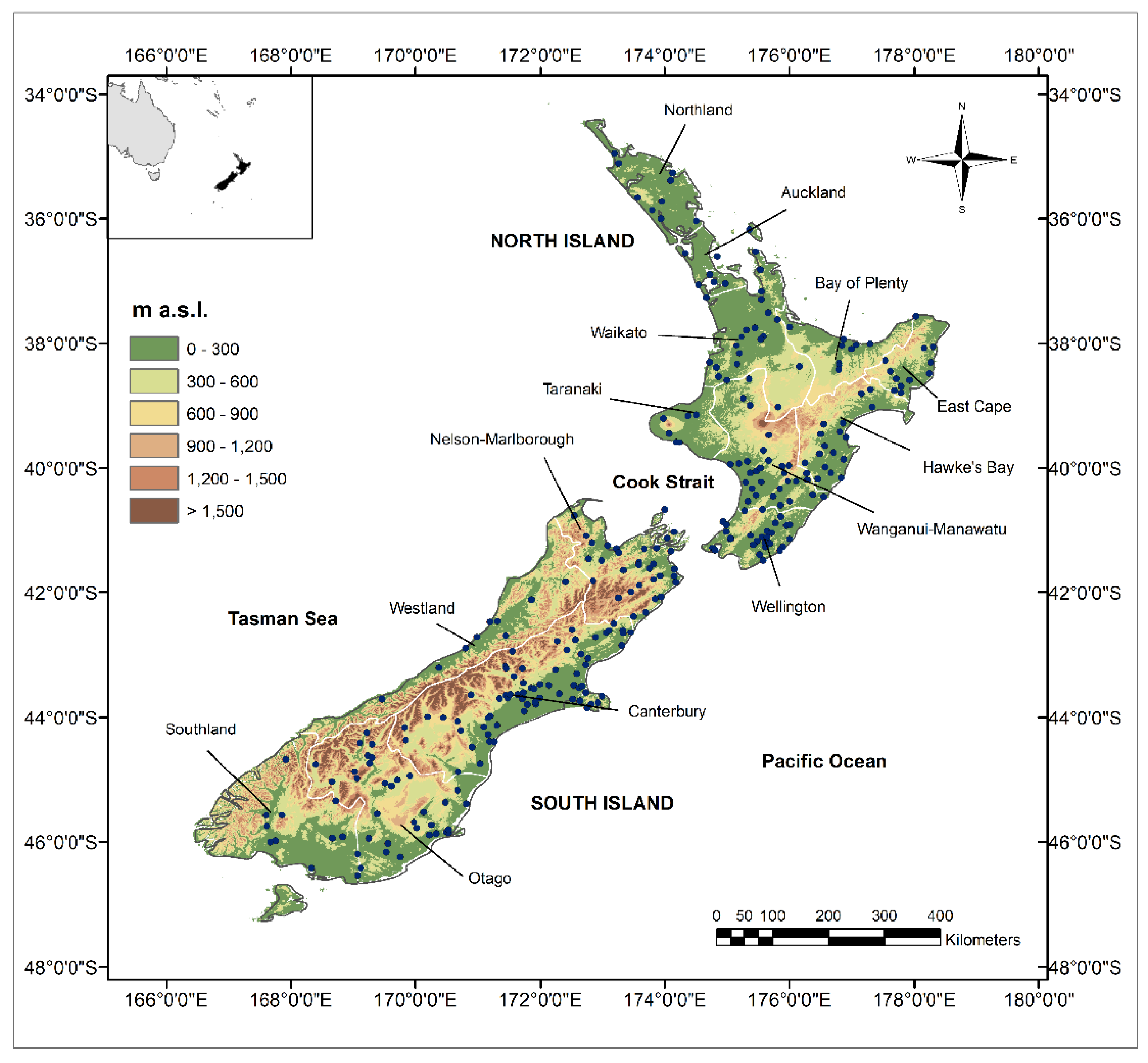
2. Study Area and Observation

New Zealand is an island country located in the southwestern Pacific Ocean, east of the Australian continent, between 34° to 47° S and between 164° to 179° E, with an area of 270,000 km². It consists of two main islands presenting a northeast-southwest oriented shape. The North Island is mainly characterized by plains but it also presents mountains reaching a maximum altitude of more than 2700 m a.s.l. Conversely, the South Island is mainly mountainous, with the Southern Alps reaching an altitude of 3764 m (Figure 1).

Generally, New Zealand’s weather patterns reflect those of the oceanic mid-latitude locations [36,37], but it is also affected by some physical factors [38]. The first factor is the location of the country in the Pacific Ocean, which influences air circulation and seasonal climate. The air masses coming from the tropical zones of the Pacific lead to a humid weather, with fresh summers and mild winters, and temperatures oscillating between 18 °C and 21 °C, although snow and frost occur as a consequence of the oceanic currents from Antarctica. The presence of the mountains in the eastern side of the North Island and of the 750-km long, over 3000-m high Southern Alps traversing the South Island constitutes the second factor affecting air circulation and determining New Zealand’s climate [39,40]. As a result, large differences in the rainfall volumes occur even over short distances between the mountain areas and the eastward plans. Moreover, summers in the northern part of the North Island are influenced by the westerly wind perturbations [38]. Finally, although more than 2000 km divide New Zealand from the Australian continent, this significantly influences New Zealand seasonal climate because of the cyclogenesis region moving through the Tasman Sea which is responsible for the significant differences in the precipitation amount occurring over short distances especially in the South Island [41,42,43,44]. Clear sky conditions in winter lead to considerable surface cooling, which, in turn, results in stable lower atmospheric conditions. This has an impact eastward since it prevents the western airflow from significantly affecting New Zealand. On the contrary, large convective hot air masses coming across the Tasman Sea cause robust airflows affecting New Zealand in summer [25].

New Zealand’s climate has been carefully described by The National Institute of Water and Atmosphere Research (NIWA) of New Zealand [45]. According to NIWA, warm, humid summers and mild winters affect the North Island, in which winter is the rainiest period of the year, while summer and autumn are characterized by tropical storms and intense precipitation. The Central Region of the North Island is the least affected by winds that heavily sweep many areas of the country. Stable, dry, and warm summers with unstable cool winters are typical of this region. The south-west part of the North Island does not present many climate extremes with a stable weather in summer, which is usually warm, and at the beginning of autumn and unsettled, although not very cold, winters. The sunniest area of New Zealand is the northern part of the South Island, characterised by warm, dry and stable summer. In the western side of the South Island is affected by extreme yearly precipitation higher than average, although occasional dry spells my occur between the end of the summer and the winter months. The eastern and inland areas of the South Island are characterized by low mean annual rainfall and by long dry episodes in the summer season.

With the aim to perform a spatial analysis of the rainfall in New Zealand, monthly observations have been extracted from the NIWA database for the period 1951–2012. Several studies on New Zealand climate [36,46,47,48,49,50] made extensive use of this database, which has been acknowledged as a high-quality database with almost complete records. In 2012 the original database included monthly observation from 3011 rain gauges (1 station per 89 km²). In order to perform a reliable analysis, in this study only the stations working in 2012, with more than 50 years of observation and less than 5% of missing data have been considered. As a result of this preliminary check a final database of monthly observation from 294 rain gauges (1 station per 913 km²) has been considered (Figure 1).

3. Methodology

With the aim to determine the best technique in reproducing the actual surface, both deterministic and geostatistical algorithms were applied to generate the rainfall maps of New Zealand at a monthly scale. The performance of each method was evaluated. All the procedures mentioned above have been implemented in an R statistical computing environment, mainly using the ‘gstat’ package [51].

3.1. The Inverse Distance Weighting (IDW)

One of the most popular and adopted deterministic methods in reproducing the actual surface is the IDW [52], which is a non-linear interpolation technique that considers the measured values in neighbouring points to evaluate a value for any unmeasured location. A neighbourhood about the interpolated point is identified and a weighted average is taken of the observation values within this neighbourhood. The weights are a decreasing function of distance computed as follows.

$${\widehat{v}}_i=\frac{{\displaystyle \sum _{i=1}^n\frac{1}{d^p{}_i}{v}_i}}{{\displaystyle \sum _{i=1}^n\frac{1}{d^p{}_i}}},$$

(1)

where ${\widehat{v}}_i$ is the value to be estimated, $v_i$ is the known value, $d^p{}_i\dots ,d^p{}_n$ are distances from n data points to the power of p of the point estimated.

The lower the exponent, the more uniformly all neighbours are incorporated into the calculation (regardless of their distance), and therefore, the “smoother” the estimated surface. The higher the exponent, the more accentuated and “unsettled” is the surface because only the nearest neighbours’ weight is integrated into the interpolation.

To minimise the interpolation errors, a power value of 2 for monthly time steps has been performed and applied in the estimation for IDW.

3.2. Geostatistical Methods

Although the IDW is largely applied, it lacks any direction-specific (anisotropic) information, thus ignoring the spatial correlations which are not incorporated into the estimation. In some scientific contributions, the IDW was used as a basic approach (i.e., a reference) to assess the spatial prediction [53]. This weakness does not occur in geostatistical approach. For interested readers a detailed presentation of geostatistical theories can be found in [26,54,55,56]. Usually the spatial interpolation is performed by using a weight of observed regionalised values to evaluate a regionalised value in unmeasured points. Kriging is a widely used interpolation technique that takes into account the spatial dependent correlation of environmental variables assigning more weight to neighbouring points [56]. Kriging also provides an uncertainty estimate. Semi-variogram modelling [57] is the first and the key step between spatial description and spatial prediction in kriging computation. After computing the empirical semi-variogram, for all pairs of locations in a given distance, this is fitted with a theoretical model, which is a function of the lag of data pair values, that is used to evaluate the weight by means of the different equation systems of the several krigings: ordinary kriging (OK), kriging with an external drift (KED), and cokriging (COK). In this study, we did not provide local variograms, considering that, as demonstrated by Lloyd [53], their use leads to a small reduction in prediction errors.

3.2.1. Ordinary Kriging (OK)

Ordinary kriging is the most popular kriging interpolator. It provides an estimate of the value of the random variable Z(x) at an unsampled point x₀ based on the weighted average of observed neighbouring points Z(x_α) within a specific area [56]:

$$Z_{OK}^{*}\left(x_0\right)={\displaystyle \sum _{\alpha =1}^{n\left(x_0\right)}{\lambda }_{\alpha }^{OK}z\left(x_{\alpha }\right)},$$

(2)

where λ_α are the ordinary kriging weights and n(x₀) is the number of measured values of pairs of points multiplied by their spatial distance h. The weights are obtained so that the estimate is unbiased and the variance is minimised.

3.2.2. Kriging with an External Drift (KED)

In geostatistics, the kriging with an external drift (KED) method allows the use of auxiliary information, available at all locations, which has an effect on the local spatial trend of the dependent variable. So, the predictions are made as with kriging, with the difference that the covariance matrix of residuals is extended with the auxiliary predictors.

The secondary variable’s spatial behaviour is similar to an indicator of the general trend typical of predictions’ representation. In this study, the KED method was applied because it allows incorporation of the elevation and geographic coordinates as the secondary variables. This choice is in accordance with the rainfall observation analysed, which have a global elevation-controlled trend in the south-western to north-east direction.

Let z(x) be the external deterministic variable. The model for the random function is:

$$Y\left(x\right)=a+b.z\left(x\right)+Y_R\left(x\right),$$

(3)

where Y_R(x) is a residual stationary random field, z(x) is known everywhere and a and b are coefficients to be estimated if Y_R(x) is needed. Kriging of Y at a location x₀ where it is unknown is a linear combination of the data:

$$Y^{*}\left(x_0\right)={\displaystyle \sum _{i=1}^n{\lambda }_i}\left(x_i\right),$$

(4)

where the Y(x_i)’s are the values at the n measured sites and the λ_i’s solve the following kriging system:

$$\{\begin{array}{l}{\displaystyle \sum _{j=1}^n{\lambda }_{j}C\left(x_i-x_j\right)-{\mu }_1-{\mu }_{2}z\left(x_i\right)=C\left(x_i-x_0\right)fori=1,\dots ,n}\\ {\displaystyle \sum _{i=1}^n{\lambda }_i=1}\\ {\displaystyle \sum _{j=1}^n{\lambda }_{i}z\left(x_i\right)=z\left(x_0\right)}\end{array},$$

(5)

The KED requires a less demanding semivariogram analysis compared to OK which requires a semivariogram for each of the covariates.

The last constraint is added so that the linear predictor Y*(x₀) filters the effect of the external drift, μ₁ and μ₂ are the Lagrange multipliers that account for the unbiasedness constraints with the minimal prediction variance.

3.2.3. Ordinary Cokriging (COK)

The last methodology applied in the present study is ordinary cokriging (COK). It offers additional advantages over ordinary kriging. It involves the use of a secondary variable (covariate) that is cross-correlated with the primary or sample variable of interest. The secondary variable is usually sampled more frequently and regularly, thus allowing estimation of unknown points using both variables ‘globally’ for the mean of all estimates but also ‘conditionally’ for the estimates within individually specified grade categories. This can aid in minimizing the error variance of the estimation.

3.3. Cross-Validation

The process of deciding whether the numerical results quantified by different interpolators are acceptable as descriptions of the data, is known as cross-validation, which tests the model’s capability to predict data. Performing the cross-validation, some of the data are removed before training begins. Then when training is done, the data that were removed can be used to test the performance of the learned model on “new” data. The actual error incurred in this process is measured by the difference between the actual and estimated value [58,59,60].

The accuracy of calculation was measured by the mean absolute error (MAE) and the root-mean-square error (RMSE). The MAE and RMSE are calculated for the data set as:

$$MAE=\frac{1}{n}{\displaystyle \sum _{i=1}^n\left|e_i\right|},$$

(6)

$$RMSE=\sqrt{\frac{1}{n}{\displaystyle \sum _{i=1}^n{e}_i^2}},$$

(7)

where $\left|e_i\right|=\left|y_i-{\widehat{y}}_i\right|$, actual = $y_i$, and predicted = ${\widehat{y}}_i$.

The closer the values of RMSE are to zero the more accurate the model results will be.

The RMSE value cannot be considered a performance criterion to define the reliability of the kriging estimate [12], even if it is used in all geostatistical methods. Many studies regarding spatial interpolation of rainfall [34], evaluation of the best interpolation methods for mapping climatic variables at regional scale [61], and spatial distribution of rainfall [62] have performed the MAE and RMSE calculation in order to compare the results. A graphical result of the goodness of fitting actual and estimated values is given by the scatterplot: the closer its slope is 1, the more accurate the estimation is.

4. Results and Discussion

In this section, a comparison of the results obtained through deterministic and geostatistical algorithms is presented. In

Table 1. Descriptive statistics of the monthly precipitation observation for the 294 rainfall series.

Month	Mean	Median	Max	Min	CV	SK	KU
January	90.0	77.3	632.6	36.9	0.66	5.21	35.06
February	83.2	73.9	512.0	27.9	0.58	4.52	29.42
March	94.4	80.9	609.7	40.8	0.60	4.81	33.29
April	98.2	88.4	547.5	35.9	0.57	3.74	20.67
May	113.0	102.9	553.5	31.8	0.54	3.09	14.98
June	113.8	106.0	439.5	25.8	0.53	1.90	6.31
July	117.4	111.8	380.0	20.4	0.49	1.41	3.42
August	110.9	101.7	433.5	21.4	0.52	1.92	6.03
September	98.9	85.6	542.3	26.5	0.64	3.42	16.52
October	106.2	91.3	612.0	37.4	0.66	3.96	20.34
November	94.5	79.7	573.3	34.5	0.66	4.27	23.48
December	101.8	88.7	595.5	37.2	0.61	4.26	23.93

CV = Coefficients of variation; SK = Coefficient of skewness; KU = Kurtosis.

, the results of the exploratory statistical analysis of monthly rainfall are shown. Mean monthly rainfall ranges between 83.2 mm (February) and 117.4 mm (July). The maximum and the minimum monthly values have been detected in January (632.6 mm) and in July (20.4 mm), respectively.

The coefficients of variation evaluated for the monthly rainfall values range between 49% and 66%, thus evidencing a low spatial heterogeneity of rainfall in New Zealand (Table 1). The exploratory statistical analysis of the precipitation observation was mainly performed to evaluate whether the monthly values fit a normal distribution. Indeed normality is a desirable property for kriging, that will generate the best absolute estimate only if the random function fits a normal distribution [30]. As a result, appreciably different monthly mean and median values and high values of skewness coefficients were observed (Table 1). Therefore, a priori logarithmic transformation of the data was performed after which normality was obtained (similar mean and median values and close to zero values of the coefficients of skewness).

Due to the station density, 1 station per 913 km², the spatial variability has been considered to be equal in the different directions, and thus an omnidirectional semi-variograms, evaluated for the monthly rainfall observation, has been considered to carried out the spatial dependence analysis. To represent the empirical semivariogram by fitting a theoretical model, it was found that using a combination of theoretical models results in a more accurate fit onto the empirical semivariance than using a single model. Therefore, the semivariance of three models, precisely Gaussian, spherical, and circular, were used to fit the empirical semivariograms of monthly rainfall observation and for avoidance of negative interpolations. For all cases, two models combined showed the best fittings. The results of variograms parameters are different for each month (not shown). An example of experimental semi-variograms and their fitted models for the three geostatistical methods, computed for June, is shown in Figure 2.

In order to match the interpolation performance of the adopted algorithms, the cross-validation has been applied. The cross-validation results (scatter plots of predicted versus measured values) for June are shown for the four methods in Figure 2.

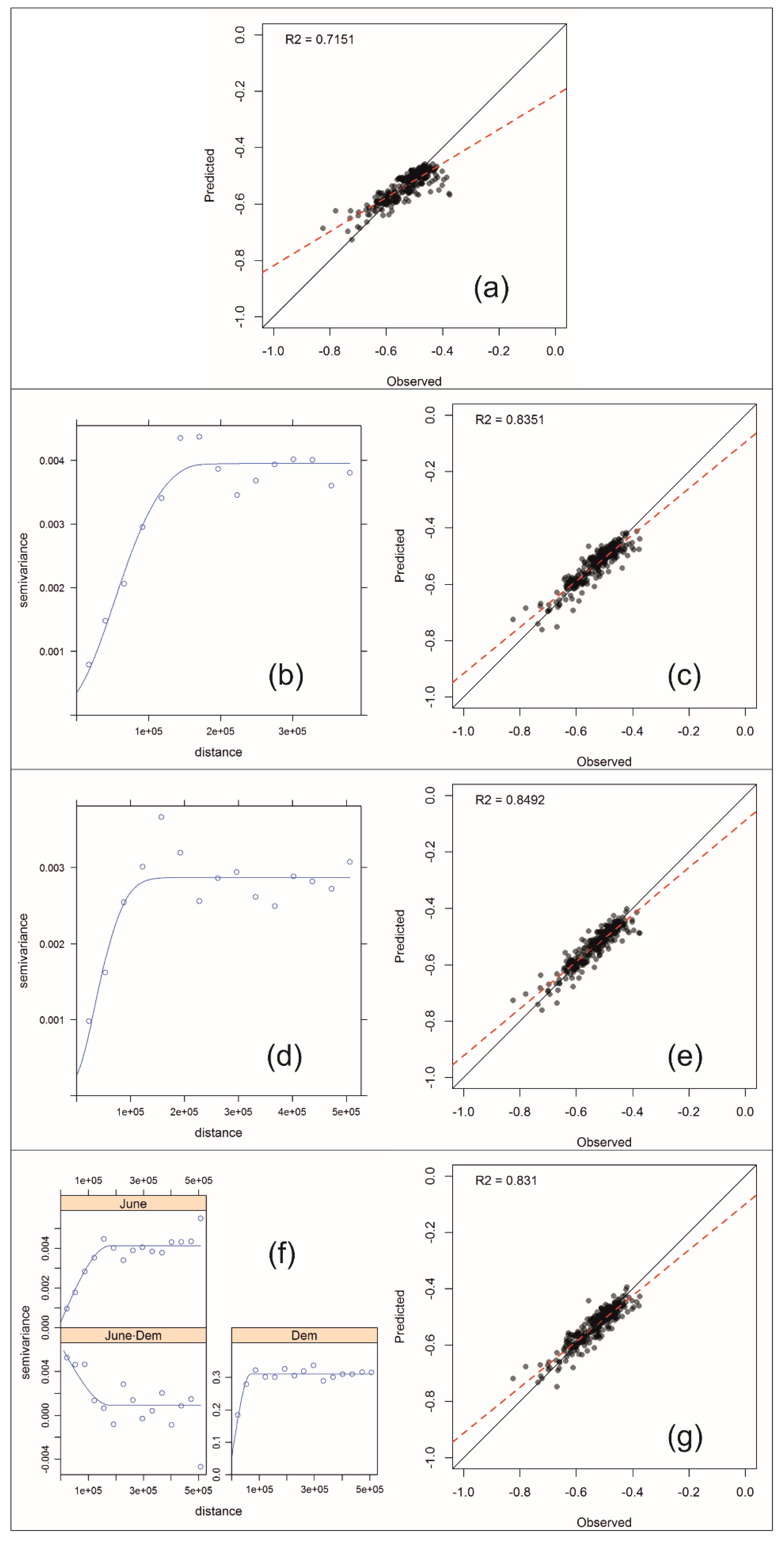
4.1. The Inverse Distance Weighting (IDW)

For the IDW interpolation, which uses a simple algorithm based on distance, the closest measured values had the most influence. Typically, the spatial distribution evaluated with this method showed marked areas in correspondence of the high or low rainfall values (Figure 3). In fact, generally, this method produces spikes around the measured points [63], although it can depict well local detailed changing as shown by Shi et al. [64]. On the other hand, Chen and Liu [65], using IDW in estimating the spatial distribution of rainfall in the middle of Taiwan, obtained an higher accuracy in the dry season, also revealing a better ability of this estimator to predict the spatial distribution of small events.

For the several months, the coefficient of determination (R²) of the IDW of measured versus predicted rainfall, showed the lowest values among the different interpolation methods, ranging between 0.5318 and 0.7324 (Figure 2 and

Table 2. Coefficient of determination (R²) of measured versus predicted monthly rainfall for the different interpolation methods (inverse distance weighting, IDW; ordinary kriging, OK; kriging with an external drift, KED; ordinary cokriging, COK).

Month	IDW	OK	KED	COK
January	0.5393	0.6375	0.7021	0.7089
February	0.5329	0.6406	0.6711	0.6816
March	0.5318	0.6551	0.6901	0.7098
April	0.6178	0.7449	0.7748	0.7921
May	0.6266	0.7515	0.7748	0.7766
June	0.7151	0.8236	0.8492	0.8486
July	0.7324	0.8277	0.8320	0.8332
August	0.7043	0.8074	0.8194	0.8408
September	0.6569	0.7825	0.7956	0.8055
October	0.6097	0.7459	0.7723	0.7900
November	0.5712	0.6963	0.7168	0.7422
December	0.5562	0.6811	0.7064	0.7319

). Moreover, as a consequence of the cross-validation test, this method did not result, in any analysed month, the best interpolating rainfall method (

Table 3. Best interpolation method (inverse distance weighting, IDW; ordinary kriging, OK; kriging with an external drift, KED; ordinary cokriging, COK) based on the cross-validation test (mean absolute error, MAE; root-mean-square error, RMSE).

Month	MAE	RMSE
January	COK	COK
February	COK	COK
March	COK	COK
April	KED	KED
May	KED	COK
June	KED	COK
July	KED	COK
August	COK	COK
September	COK	COK
October	COK	COK
November	COK	COK
December	COK	COK

).

4.2. Ordinary Kriging (OK)

The ordinary kriging maps are more smoothed than the maps by IDW, especially for maximum and minimum rainfall values representations (Figure 4). Compared to the others geostatistical methods, lower results for OK were achieved by correlation coefficients of measured versus predicted monthly rainfall, particularly for the wettest months, June (0.8236), July (0.8277), and August (0.8074) (Figure 2 and Table 2).

Considering that the OK method tends to underestimate mean rainfall values, as well as IDW, it is not the best interpolator for spatially analysing the rainfall observation in any considered month. It is confirmed by the MAE and RMSE results.

4.3. Kriging with an External Drift (KED)

Improvements to accuracy for monthly rainfall interpolations in KED approach were realized by the use of elevation, extracted from a digital elevation model, and geographic coordinates as the secondary information. In the area without data, elevation, mainly extracted from a DEM, represents easily available data, which can be used to be incorporated into multivariate geostatistics of rainfall. A minimal improvement in the interpolation accuracy for monthly rainfall occurred since elevation and geographic coordinates were used as secondary variables, considering that a significantly smaller error of estimates was not achieved. Figure 5 shows the rainfall maps for 12 months obtained by using the KED technique. The results of the correlation coefficients of measured versus predicted monthly rainfall, which ranging from 0.67 to about 0.85 (Figure 2 and Table 2), attest that the KED interpolator, in few months, operated better than the COK interpolator, which was, however, the best methods for most months. In fact, differently from the IDW and the OK, the MAE and RMSE results indicated that the KED method was the best approach in some autumn and winter months (Table 3).

4.4. Ordinary Cokriging (COK)

A comparison between the use of secondary information, such as elevation, both in KED and COK interpolators, confirms that the accuracy improvement was not reached considering the error of estimates. Consequently, although adding secondary variables can increase precision, in the case study the produced maps by COK are similar to those obtained by KED and OK. Figure 6 shows the rainfall maps for 12 months obtained by using the COK technique. Therefore, as already evidenced in previous studies [12] and confirmed in this one, when the correlation between rainfall and elevation is too small, the advantages derived by using multivariate techniques is negligible. The values of the correlation coefficients of measured versus predicted monthly rainfall ranged between 0.68 and 0.84 (Figure 2 and Table 2). The COK interpolator can be evaluated as the best approach to analysing rainfall observation in many analysed months (Table 3) as confirmed by the MAE and the RMSE results.

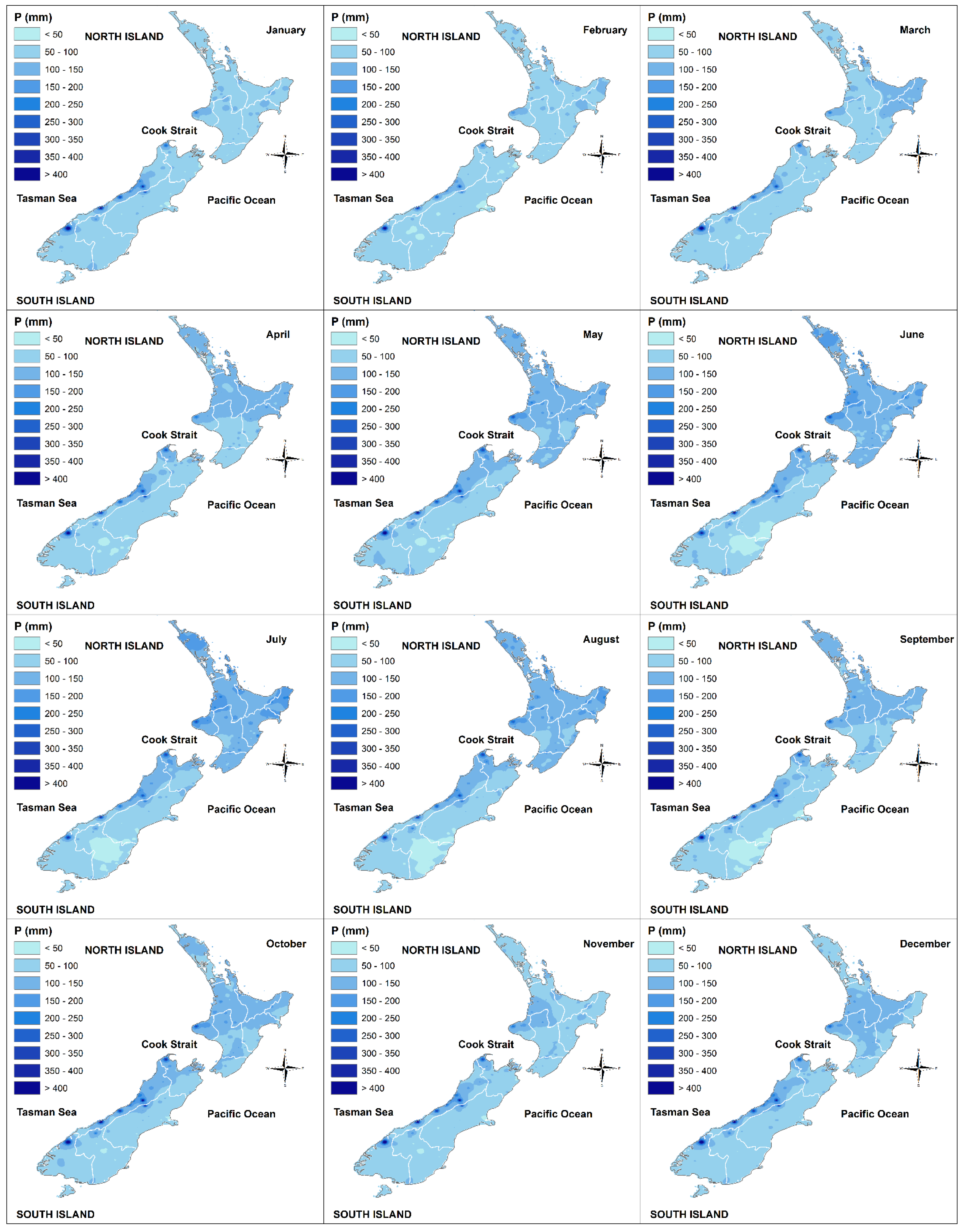
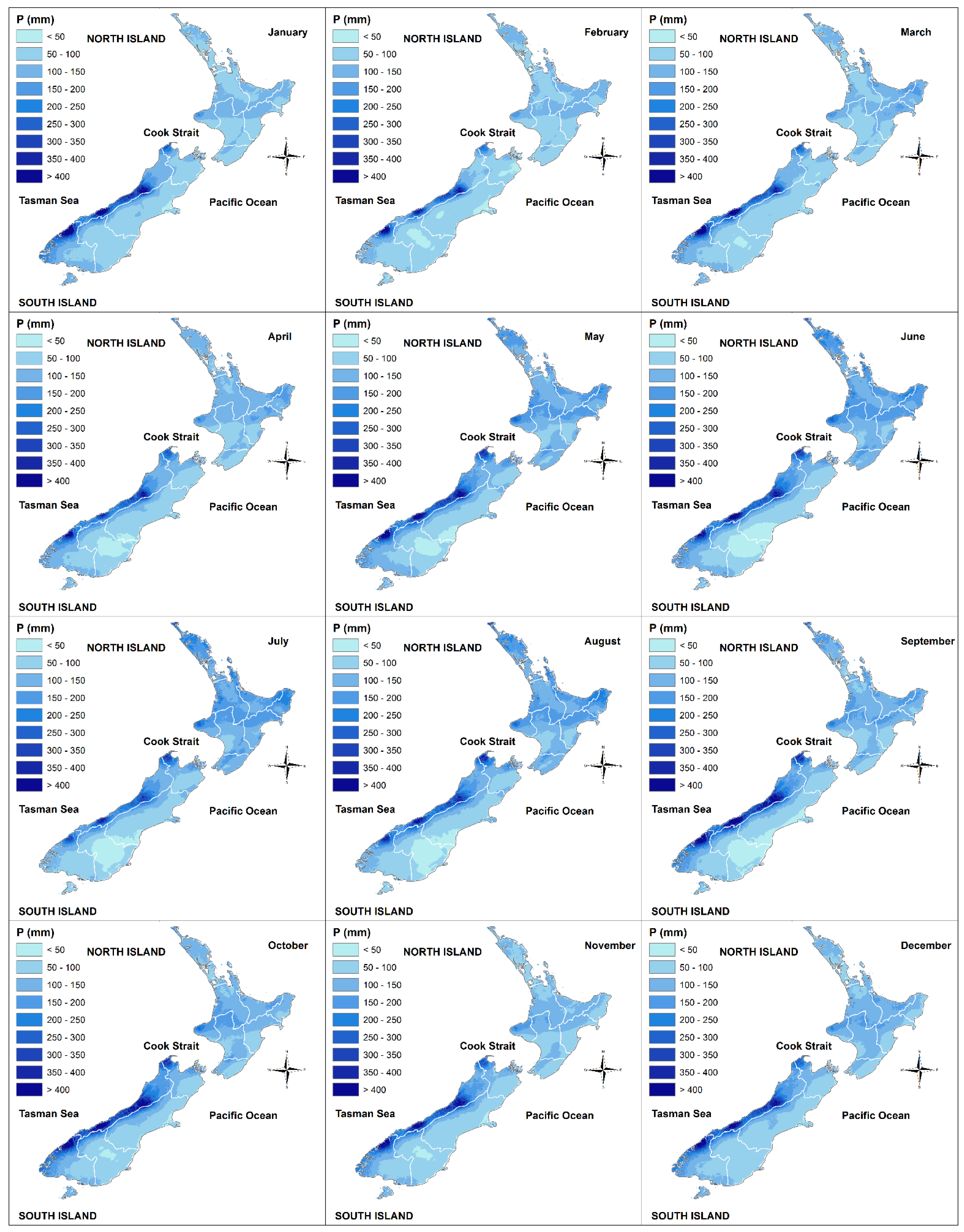
4.5. Comparison of the Interpolation Methods

The analysis of deterministic and geostatistical methods allowed to identify strengths and weaknesses of the applicability of the different algorithms to monthly rainfall in New Zealand. Since IDW considers only the distance between estimated and sampled points and leaves out the pattern of spatial dependence of rainfall observation, as expected, substantially different results have been obtained by applying the IDW and the geostatistical methods.

In Table 3 results of the cross-validation are shown in terms of MAE and RMSE values, providing clear indications of the effectiveness of kriging in the spatial interpolation of monthly rainfall observation in New Zealand. In fact, the IDW technique has been clearly outperformed by the geostatistical approaches, thus confirming past studies (e.g., [12,63]) which found IDW to be less accurate than geostatistical interpolators in the estimation of monthly and annual rainfall.

Specifically, considering the RMSE, the COK has been identified as the most accurate interpolator in 11 months with the exception of April when the KED resulted more precise. However, taking into account the MAE, the KED has been identified as the most accurate interpolator in April, May, June and July, and the COK in the remaining months. The COK can be thus indicated as the best method for the spatial interpolation of rainfall in New Zealand for almost all months. The IDW and OK methods were not the best approaches for interpolating rainfall in any analysed month. Overall, the COK evidenced the best least bias and scatter in the cross-validation test, with the lowest errors. Finally, interesting results can be obtained from the visual comparison among the maps obtained from the application of the different geostatistical interpolation algorithms. In fact, similar rainfall spatial distributions, have been produced with the geostatististical interpolators, and all these distributions seem to be consistent with natural precipitation. In particular, as demonstrated in previous studies [12,14,53,66,67,68], adding elevation and geographical coordinates as secondary variables in the application of the KED and the COK, did not lead to a significant improvement of the results, that is explainable considering the weak correlation identified between precipitation and the secondary variables. In fact, as pointed out by Goovaerts [12], better results of the COK with respect to the OK can be observed with an increase in the correlation between precipitation and altitude. Moreover, Goovaerts [26] evidenced that the impact of the auxiliary data on the COK interpolations generally depends on the correlation between primary and secondary variables but also on their spatial continuity patterns. Perhaps, as suggested by Kyriakidis et al. [66], using monthly time series of covariates (e.g., monthly wind speed or humidity) as additional information in the KED and the COK instead of variables fixed in time (e.g., topography and geographical coordinates) can lead to a much better cross-validation than those obtained by the OK. Unfortunately, these variables are available in New Zealand only for short observation periods and in very few stations.

5. Conclusions

Agriculture in New Zealand is the largest sector of the tradable economy; consequently, knowledge of the spatial distributions of rainfall in this country is essential for water resource management. In fact, New Zealand presents large spatial differences in the rainfall distribution. As an example, although the Southern Alps are one of the rainiest places in the world, the east side of the South Island often suffers from droughts. Moreover, sustainable landscape management requires spatially interpolated data, whose outcomes are strictly related to models and geostatistical parameters adopted.

In this paper, in order to generate precipitation maps at monthly scale, both deterministic (inverse distance weighting) and geostatistical (ordinary kriging, kriging with an external drift, and ordinary cokriging) methodologies have been applied and the prediction performance of each method was evaluated through cross-validation and visual examination of the precipitation maps produced. Results of the cross-correlation confirmed the worse accuracy of IDW than geostatistical methods. In particular, although the COK has been identified as the best method in the interpolation of monthly rainfall in New Zealand, the visual comparison of the spatial results obtained with the different geostatistical methods evidenced similar rainfall distributions, thus demonstrating that no significant results have been achieved by adding elevation and geographical coordinates as secondary variables. Further analysis could be conducted to improve the spatial distribution of monthly rainfall by adding new secondary variables, such as wind speed or humidity.

References

1. Buttafuoco, G.; Caloiero, T.; Guagliardi, I.; Ricca, N. Drought assessment using the reconnaissance drought index (RDI) in a southern Italy region. In Proceedings of the 6th IMEKO TC19 Symposium on Environmental Instrumentation and Measurements, Reggio Calabria, Italy, 24–26 June 2016; pp. 52–55. [Google Scholar]
2. Frazier, A.G.; Giambelluca, T.W.; Diaz, H.F.; Needham, H.L. Comparison of geostatistical approaches to spatially interpolate month-year rainfall for the Hawaiian Islands. Int. J. Climatol. 2016, 36, 1459–1470. [Google Scholar] [CrossRef] [Green Version]
3. Ly, S.; Charles, C.; Degré, A. Geostatistical interpolation of daily rainfall at catchment scale: The use of several variogram models in the Ourthe and Ambleve catchments, Belgium. Hydrol. Earth Syst. Sci. 2011, 15, 2259–2274. [Google Scholar] [CrossRef] [Green Version]
4. Ricca, N.; Guagliardi, I. Multi-temporal dynamics of land use patterns in a site of community importance in southern Italy. Appl. Ecol. Environ. Res. 2015, 13, 677–691. [Google Scholar] [CrossRef]
5. Caloiero, T.; Caloiero, P.; Frustaci, F. Long-term precipitation trend analysis in Europe and in the Mediterranean basin. Water Environ. J. 2018, 32, 433–445. [Google Scholar] [CrossRef]
6. Rosas, Y.M.; Peri, P.L.; Lencinas, M.V.; Lasagno, R.; Martínez Pastur, G.J. Improving the knowledge of plant potential biodiversity-ecosystem services links using maps at the regional level in Southern Patagonia. Ecol. Process. 2021, 10, 53. [Google Scholar] [CrossRef]
7. Dhamodaran, S.; Lakshmi, M. Comparative analysis of spatial interpolation with climatic changes using inverse distance method. J. Ambient Intell. Humaniz. Comput. 2021, 12, 6725–6734. [Google Scholar] [CrossRef]
8. Hadri, A.; Saidi, M.E.M.; Saouabe, T.; El Alaoui El Fels, A. Temporal trends in extreme temperature and precipitation events in an arid area: Case of Chichaoua Mejjate region (Morocco). J. Water Clim. Chang. 2021, 12, 895–915. [Google Scholar] [CrossRef]
9. Delbari, M.; Afrasiab, P.; Jahani, S. Spatial interpolation of monthly and annual rainfall in northeast of Iran. Meteorol. Atmos. Phys. 2013, 122, 103–113. [Google Scholar] [CrossRef]
10. Rata, M.; Douaoui, A.; Larid, M.; Douaik, A. Comparison of geostatistical interpolation methods to map annual rainfall in the Chéliff watershed, Algeria. Theor. Appl. Climatol. 2020, 141, 1009–1024. [Google Scholar] [CrossRef]
11. Mirás-Avalos, J.M.; Paz-González, A.; Vidal-Vázquez, E.; Sande-Fouz, P. Mapping monthly rainfall data in Galicia (NW Spain) using inverse distances and geostatistical methods. Adv. Geosci. 2007, 10, 51–57. [Google Scholar] [CrossRef] [Green Version]
12. Goovaerts, P. Geostatistical approaches for incorporating elevation into the spatial interpolation of rainfall. J. Hydrol. 2000, 228, 113–129. [Google Scholar] [CrossRef]
13. Zhang, G.; Su, X.; Ayantobo, O.O.; Feng, K.; Guo, J. Spatial interpolation of daily precipitation based on modified ADW method for gauge-scarce mountainous regions: A case study in the Shiyang River Basin. Atmos. Res. 2021, 247, 105167. [Google Scholar] [CrossRef]
14. Pellicone, G.; Caloiero, T.; Modica, G.; Guagliardi, I. Application of several spatial interpolation techniques to monthly rainfall data in the Calabria region (southern Italy). Int. J. Climatol. 2018, 38, 3651–3666. [Google Scholar] [CrossRef]
15. Hurtado, S.I.; Zaninelli, P.G.; Agosta, E.A.; Ricetti, L. Infilling methods for monthly precipitation records with poor station network density in Subtropical Argentina. Atmos. Res. 2021, 254, 105482. [Google Scholar] [CrossRef]
16. Di Piazza, A.; Lo Conti, F.; Noto, L.V.; Viola, F.; La Loggia, G. Comparative analysis of different techniques for spatial interpolation of rainfall data to create a serially complete monthly time series of precipitation for Sicily, Italy. Int. J. Appl. Earth Obs. Geoinf. 2011, 13, 396–408. [Google Scholar] [CrossRef]
17. Xu, W.; Zou, Y.; Zhang, G.; Linderman, M. A comparison among spatial interpolation techniques for daily rainfall data in Sichuan Province, China. Int. J. Climatol. 2015, 35, 2898–2907. [Google Scholar] [CrossRef]
18. Li, J.; Heap, A.D. A review of comparative studies of spatial interpolation methods in environmental sciences: Performance and impact factors. Ecol. Inform. 2011, 6, 228–241. [Google Scholar] [CrossRef]
19. Agnew, M.; Palutikof, J. GIS-based construction of baseline climatologies for the Mediterranean using terrain variables. Clim. Res. 2000, 14, 115–127. [Google Scholar] [CrossRef] [Green Version]
20. Vicente-Serrano, S.; Saz-Sánchez, M.; Cuadrat, J. Comparative analysis of interpolation methods in the middle Ebro Valley (Spain): Application to annual precipitation and temperature. Clim. Res. 2003, 24, 161–180. [Google Scholar] [CrossRef] [Green Version]
21. Hutchinson, M.F.; Gessler, P.E. Splines—More than just a smooth interpolator. Geoderma 1994, 62, 45–67. [Google Scholar] [CrossRef]
22. Legates, D.R.; Willmott, C.J. Mean seasonal and spatial variability in global surface air temperature. Theor. Appl. Climatol. 1990, 41, 11–21. [Google Scholar] [CrossRef]
23. Mair, A.; Fares, A. Comparison of Rainfall Interpolation Methods in a Mountainous Region of a Tropical Island. J. Hydrol. Eng. 2011, 16, 371–383. [Google Scholar] [CrossRef]
24. de A. Borges, P.; Franke, J.; da Anunciação, Y.M.T.; Weiss, H.; Bernhofer, C. Comparison of spatial interpolation methods for the estimation of precipitation distribution in Distrito Federal, Brazil. Theor. Appl. Climatol. 2016, 123, 335–348. [Google Scholar] [CrossRef]
25. Chen, T.; Ren, L.; Yuan, F.; Yang, X.; Jiang, S.; Tang, T.; Liu, Y.; Zhao, C.; Zhang, L. Comparison of Spatial Interpolation Schemes for Rainfall Data and Application in Hydrological Modeling. Water 2017, 9, 342. [Google Scholar] [CrossRef] [Green Version]
26. Goovaerts, P. Geostatistics for Natural Resources Evaluation; Oxford University Press: New York, NY, USA, 1997. [Google Scholar]
27. Isaaks, E.H.; Srivastava, R.M. An Introduction to Applied Geostatistics; Oxford University Press: New York, NY, USA, 1989. [Google Scholar]
28. Goovaerts, P. Using elevation to aid the geostatistical mapping of rainfall erosivity. CATENA 1999, 34, 227–242. [Google Scholar] [CrossRef]
29. Journel, A.G.; Huijbregts, C.J. Mining Geostatistics; Academic Press: London, UK; New York, NY, USA, 1978. [Google Scholar]
30. Moral, F.J. Comparison of different geostatistical approaches to map climate variables: Application to precipitation. Int. J. Climatol. 2010, 30, 620–631. [Google Scholar] [CrossRef]
31. Phillips, D.L.; Dolph, J.; Marks, D. A comparison of geostatistical procedures for spatial analysis of precipitation in mountainous terrain. Agric. For. Meteorol. 1992, 58, 119–141. [Google Scholar] [CrossRef]
32. Tabios, G.Q.; Salas, J.D. A comparative analysis of techniques for spatial interpolation of precipitation. J. Am. Water Resour. Assoc. 1985, 21, 365–380. [Google Scholar] [CrossRef]
33. Tsintikidis, D.; Georgakakos, K.P.; Sperfslage, J.A.; Smith, D.E.; Carpenter, T.M. Precipitation Uncertainty and Raingauge Network Design within Folsom Lake Watershed. J. Hydrol. Eng. 2002, 7, 175–184. [Google Scholar] [CrossRef]
34. Dirks, K.N.; Hay, J.E.; Stow, C.D.; Harris, D. High-resolution studies of rainfall on Norfolk Island. J. Hydrol. 1998, 208, 187–193. [Google Scholar] [CrossRef]
35. Zou, W.; Yin, S.; Wang, W. Spatial interpolation of the extreme hourly precipitation at different return levels in the Haihe River basin. J. Hydrol. 2021, 598, 126273. [Google Scholar] [CrossRef]
36. Dravitzki, S.; McGregor, J. Extreme precipitation of the Waikato region, New Zealand. Int. J. Climatol. 2011, 31, 1803–1812. [Google Scholar] [CrossRef]
37. Garnier, B. New Zealand Weather and Climate; Whitcombe and Tombs Ltd.: Christchurch, NZ, USA, 1950. [Google Scholar]
38. Oliver, J.E. (Ed.) Encyclopedia of World Climatology; Springer: Dordrecht, The Netherlands, 2005; ISBN 978-1-4020-3266-0. [Google Scholar]
39. Griffiths, G. Drivers of extreme daily rainfalls in New Zealand. Weather Clim. 2011, 31, 24. [Google Scholar] [CrossRef]
40. Jiang, N.; Griffiths, G.; Lorrey, A. Influence of large-scale climate modes on daily synoptic weather types over New Zealand. Int. J. Climatol. 2013, 33, 499–519. [Google Scholar] [CrossRef]
41. Sinclair, M.R. An Objective Cyclone Climatology for the Southern Hemisphere. Mon. Weather Rev. 1994, 122, 2239–2256. [Google Scholar] [CrossRef]
42. Sinclair, M.R. An extended climatology of extratropical cyclones over the southern hemisphere. Weather Clim. 1995, 15, 21. [Google Scholar] [CrossRef]
43. Sinclair, M.R. A Climatology of Cyclogenesis for the Southern Hemisphere. Mon. Weather Rev. 1995, 123, 1601–1619. [Google Scholar] [CrossRef] [Green Version]
44. Trenberth, K.E. Storm Tracks in the Southern Hemisphere. J. Atmos. Sci. 1991, 48, 2159–2178. [Google Scholar] [CrossRef]
45. National Institute of Water and Atmospheric Research (NIWA) Overview of New Zealand Climate. Available online: http://www.niwa.co.nz/education-and-training/schools/resources/climate/overview (accessed on 27 February 2021).
46. Griffith, J.A.; Stehman, S.V.; Sohl, T.L.; Loveland, T.R. Detecting trends in landscape pattern metrics over a 20-year period using a sampling-based monitoring programme. Int. J. Remote Sens. 2003, 24, 175–181. [Google Scholar] [CrossRef]
47. Salinger, M.J.; Mullan, A.B. New Zealand climate: Temperature and precipitation variations and their links with atmospheric circulation 1930–1994. Int. J. Climatol. 1999, 19, 1049–1071. [Google Scholar] [CrossRef]
48. Caloiero, T. Drought analysis in New Zealand using the standardized precipitation index. Environ. Earth Sci. 2017, 76, 569. [Google Scholar] [CrossRef]
49. Caloiero, T. SPI Trend Analysis of New Zealand Applying the ITA Technique. Geosciences 2018, 8, 101. [Google Scholar] [CrossRef] [Green Version]
50. Caloiero, T. Evaluation of rainfall trends in the South Island of New Zealand through the innovative trend analysis (ITA). Theor. Appl. Climatol. 2020, 139, 493–504. [Google Scholar] [CrossRef]
51. Pebesma, E.J.; Graeler, B. Package “Gstat”: Spatial and Spatio-Temporal Geostatistical Modelling, Prediction and Simulation. Available online: https://cran.r-project.org/web/packages/gstat/index.html (accessed on 27 February 2021).
52. Lu, G.Y.; Wong, D.W. An adaptive inverse-distance weighting spatial interpolation technique. Comput. Geosci. 2008, 34, 1044–1055. [Google Scholar] [CrossRef]
53. Lloyd, C.D. Nonstationary models for exploring and mapping monthly precipitation in the United Kingdom. Int. J. Climatol. 2009, 30, 390–405. [Google Scholar] [CrossRef]
54. Chiles, J.; Delfiner, P. Geostatistics: Modeling Spatial Uncertainty; John Wiley & Sons: New York, NY, USA, 1999; ISBN 9780471083153. [Google Scholar]
55. Cressie, N. Geostatistical analysis of spatial data. In Spatial Statistics and Digital Image Analysis; National Academy Press: Washington, DC, USA, 1991; pp. 87–108. [Google Scholar]
56. Webster, R.; Oliver, M.A. Geostatistics for Environmental Scientists, 2nd ed.; Statistics in Practice; John Wiley & Sons, Ltd.: Chichester, UK, 2007; ISBN 9780470517277. [Google Scholar]
57. Matheron, G. Principles of geostatistics. Econ. Geol. 1963, 58, 1246–1266. [Google Scholar] [CrossRef]
58. Buttafuoco, G.; Guagliardi, I.; Tarvainen, T.; Jarva, J. A multivariate approach to study the geochemistry of urban topsoil in the city of Tampere, Finland. J. Geochem. Explor. 2017, 181, 191–204. [Google Scholar] [CrossRef]
59. Iovine, G.; Guagliardi, I.; Bruno, C.; Greco, R.; Tallarico, A.; Falcone, G.; Lucà, F.; Buttafuoco, G. Soil-gas radon anomalies in three study areas of Central-Northern Calabria (Southern Italy). Nat. Hazards 2017, 91, 193–219. [Google Scholar] [CrossRef]
60. Guagliardi, I.; Rovella, N.; Apollaro, C.; Bloise, A.; De Rosa, R.; Scarciglia, F.; Buttafuoco, G. Modelling seasonal variations of natural radioactivity in soils: A case study in southern Italy. J. Earth Syst. Sci. 2016, 125, 1569–1578. [Google Scholar] [CrossRef] [Green Version]
61. Attorre, F.; Alfo, M.; De Sanctis, M.; Francesconi, F.; Bruno, F. Comparison of interpolation methods for mapping climatic and bioclimatic variables at regional scale. Int. J. Climatol. 2007, 27, 1825–1843. [Google Scholar] [CrossRef] [Green Version]
62. Basistha, A.; Arya, D.S.; Goel, N.K. Analysis of historical changes in rainfall in the Indian Himalayas. Int. J. Climatol. 2009, 29, 555–572. [Google Scholar] [CrossRef]
63. Lloyd, C.D. Assessing the effect of integrating elevation data into the estimation of monthly precipitation in Great Britain. J. Hydrol. 2005, 308, 128–150. [Google Scholar] [CrossRef]
64. Shi, Y.F.; Li, L.; Zhang, L.L. Application and comparing of IDW and Kriging interpolation in spatial rainfall information. In Proceedings of the Geoinformatics 2007: Geospatial Information Science, Nanjing, China, 25–27 May 2007. [Google Scholar]
65. Chen, F.-W.; Liu, C.-W. Estimation of the spatial rainfall distribution using inverse distance weighting (IDW) in the middle of Taiwan. Paddy Water Environ. 2012, 10, 209–222. [Google Scholar] [CrossRef]
66. Kyriakidis, P.C.; Kim, J.; Miller, N.L. Geostatistical Mapping of Precipitation from Rain Gauge Data Using Atmospheric and Terrain Characteristics. J. Appl. Meteorol. 2001, 40, 1855–1877. [Google Scholar] [CrossRef]
67. Moges, S.A.; Alemaw, B.F.; Chaoka, T.R.; Kachroo, R.K. Rainfall interpolation using a remote sensing CCD data in a tropical basin—A GIS and geostatistical application. Phys. Chem. Earth Parts A/B/C 2007, 32, 976–983. [Google Scholar] [CrossRef]
68. Pellicone, G.; Caloiero, T.; Guagliardi, I. The De Martonne aridity index in Calabria (Southern Italy). J. Maps 2019, 15, 788–796. [Google Scholar] [CrossRef]
Figure 1. Geographic localisation of New Zealand and the selected 294 rain gauges (blue dots) over a digital elevation model (DEM).
Applsci 11 09566 g001
Figure 2. Scatterplots between observed and estimated monthly precipitation in June for (a) inverse distance weighting (IDW), (c) ordinary kriging (OK), (e) kriging with an external drift (KED), and (g) ordinary cokriging (COK). Related semi-variograms in June for (b) OK, (d) KED, and (f) cross-variograms in June for COK. Distance is expressed in meters. DEM stands for Digital Elevation Model.
Applsci 11 09566 g002
Figure 3. Mean monthly precipitation interpolated using inverse distance weighting (IDW) method.
Applsci 11 09566 g003
Figure 4. Mean monthly precipitation interpolated using ordinary kriging (OK) method.
Applsci 11 09566 g004
Figure 5. Mean monthly precipitation interpolated using ordinary kriging (OK) method.
Applsci 11 09566 g005
Figure 6. Mean monthly precipitation interpolated using ordinary cokriging (COK) method.
Applsci 11 09566 g006