Customized Approach to Greenhouse Gas Emissions Calculations in Railway Freight Transport

Featured Application

This proposed and verified customized approach to greenhouse gas emission calculations in railway freight transport for the automotive industry is the basis for creating a software tool to support logistic planning and decision making.

Abstract

The topic of global warming is and will continue to be a crucial topic of this millennium. Freight transport, as a producer of greenhouse gas (hereinafter GHG) emissions, makes a significant contribution to the greenhouse effect. Large supply chains and large volumes of freight transport, which imply the production of significant volumes of GHG emissions, characterize the automotive industry (hereinafter AI). Thanks to these premises, it is necessary to seek and develop tools for reducing the volume of GHG emissions produced from the logistic activities of the AI, while maintaining the required level of logistic services. The assumptions for the calculation of GHG emissions from railway freight transport (hereinafter RFT) in the AI were identified through the use of semi-structured interviewing. Available railway freight GHG emission calculators were identified and analyzed from the perspective of suitability for the AI using a comparative content analysis. The main result of this manuscript is the proposal of a fully customized approach to GHG emission calculations in RFT for the AI. This approach was proposed, applied, and verified in the form of an interpretative case study. The use of this approach can be expected in support of logistic planning and decision making.

1. Introduction

In the past several decades, global warming has become a severe issue that needs a response in order to reduce CO₂ from all sectors [1]. Due to global warming, focus is given to one of CO₂’s origins, which is the continuous increase in greenhouse gas (hereinafter GHG) emissions caused by various human activities [2]. There are a number of studies and reasons to analyze direct relationships between emission sources, air pollutant concentrations, and health end-points, e.g., Lee et al. [3]. Next to the United States, China is the second largest source of CO₂ emissions in the world [4]. Organic carbon is one of the major components of ambient PM_2.5 (particulate matter (PM) ≤ 2.5 µm in aerodynamic diameter) and a significant portion of organic carbon is from secondary organic aerosol formation; results from studies suggest that the anthropogenic origin of secondary organic carbon is dominant [5]. Epidemiological studies suggest that ambient particulate matter has significant associations with adverse respiratory and cardiovascular health effects [6]. Lee et al. [7] added that it is important to understand which emission sources contribute to elevated daily PM_2.5 levels in order to develop effective control strategies. One approach to solving this problem involves the use of green energies and the reduction of CO₂ emitted from all sectors [8]. On the other hand, it must also be stated that extensive forest fires, including wildfires, prescribed burnings, agricultural waste burnings, and domestic biofuel combustion are important sources of primary air pollutants and precursors of secondary pollutants too [9,10,11,12]. With the improvement of people’s living standards, energy consumption by the transport sector will increase dramatically and, in many areas, the environmental problems and health effects caused by the transport sector have become increasingly serious [13]. The transport sector is the second largest contributor to CO₂ emissions in the world [14]. Regarding the transportation sector, it emitted above one-fourth of global CO₂ emissions [8]. It is believed that CO₂ emissions from the transport sector are growing faster than total CO₂ emissions [15]. Freight transport is an important source of energy consumption and GHG emissions [16,17].

The authors of this manuscript closely focus on GHG emissions from railway freight transport (hereinafter RFT) in the AI. The main purpose of the manuscript is to propose a customized approach to GHG emission calculations in RFT. The AI has been the most crucial industry of the domestic economy long-term but also of the whole European Union (hereinafter EU). The transport sector contributes about 10% of the gross domestic product in the Czech Republic [18]. Many domestic and global suppliers are connected to the AI. Suppliers participating in the automotive production chain in the Czech Republic make up 23% of the Czech Republic’s industrial production [18]. Many material flows are connected to the AI (e.g., materials, car bodies, containers, finished cars), which means a lot of transport, which produces GHG emissions.

Logistics with low emissions have become a preferred aim in all transport modes, especially in the EU [19,20]. The EU is on the correct path to achieve its GHG emissions reduction goal for 2020 and yet has submitted a plan to further reduce emissions by at least 55% in 2030 [21,22,23]. Chen et al. [24] discussed and analysed the energy consumption and carbon emissions of roads and railways in China’s transport sector, and they modelled scenarios of that sector’s energy consumption and carbon emissions until 2025. Wang et al. [25] studied a reduction in emissions in the transport sector, discussed current trends between RFT and road and waterway freight transport, identified de-carbonation potentials for the transport sector, and predicted transport emissions under different scenarios. Since 2019, the rate of emissions growth has continued to decrease, with transport emissions to be reduced in the near future. Feng et al. [26] defined a concept of carbon-saving profit for studying railway freight prices and discussed a maximization model of railway freight based on an established low-carbon economy. Kaewunruen et al. [27] mentioned the importance of efficient and feasible approach development for recovering and recycling wasted rolling stocks. Krezo et al. [28] discovered that emissions from materials contribute more than nine times the CO_2e emissions of machines used in renewal projects, and in addition, that extending the lifespan of rail infrastructure assets through maintenance is beneficial in terms of reducing CO_2e emissions. Furthermore, Krezo et al. [29] examined the CO₂ impact of railway resurfacing in ballasted track bed maintenance. Kaewunruen et al. [30] assessed global warming potentials due to railway tunnel construction and maintenance.

The European standard EN 16258 Methodology for the calculation and declaration of energy consumption and GHG emissions in transport (freight and passenger) was approved by the European Committee for Standardisation in 2012 [31,32,33]. Currently, there are three main approaches to the measurement of energy consumption and produced emissions [32]: Well-to-Wheel (hereinafter WtW), Well-to-Tank (hereinafter WtT) and Tank-to-Wheel (hereinafter TtW):

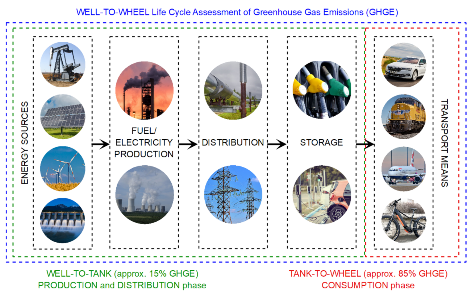
• Well-to-Wheel (the sum total of Well-to-Tank together with Tank-to-Wheel): an approach based on the monitoring of energy consumption and associated emissions production, which covers the whole process from the production of electricity or fuel, through supply to appropriate means of transport via the distribution network, to consumption associated with the operation of transport means. This approach is based on the sum of Tank-to-Wheel and Well-to-Tank values (Figure 1).
• Well-to-Tank: Energy consumption and emission production associated with energy or fuel production—this indicator covers all activities from mining of raw materials via energy or fuel production to delivery to relevant means of transport via the distribution network. This indicator does not include the mode of transport (Figure 1).
• Tank-to-Wheel: Consumption of energy and associated emissions production connected with transport means operations. This approach does not include the additional life cycle of the fuel and transport means (Figure 1).

Skrúcaný et al. [33] described a comparison of energy consumption and GHG production of three modes of transport (road, rail and water) according to current legislation—EN 16258. Another option is to use the life cycle assessment (LCA) method and a life cycle cost (LCC) analysis method [34]. These methods summarize energy consumption, GHG emissions, and costs from the perspective of the whole life cycle during the conception stage, construction stage, operation and maintenance stage, and disposal stage [34]. In some cases, the authors describe only these stages: construction, operation, maintenance, and dismantlement or demolition [1,35]. However, the authors of this manuscript, in contrast to the LCA method, focused only on the monitoring of energy consumption and associated emissions production, which covers the whole process from production of electricity or fuel, through to supply on appropriate means of transport via the distribution network, to consumption associated with the operation of transport means (WtW approach) [32]. Conception, construction, operation, maintenance, and disposal stages in connection with railway infrastructure are not included.

Reducing GHG emissions from freight transport can be achieved, for example, by supply chain pooling [36]. Supply chain logistic pooling consists of several independent companies sharing logistic activities and can be initiated for environmental reasons to optimize transportation and reduce the companies’ GHG emissions [37,38]. Lee et al. [39] stated that it is important to accurately estimate GHG emissions with their uncertainties to reduce GHG emissions and mitigate climate change. GHG emission calculators are useful tools for estimating GHG emissions and for providing information that can help to develop behavioral and policy change [40,41].

The aim of this article is to propose a fully customized approach to GHG emission calculations in RFT for the AI. The aim of this article also supports the fact that the AI has global impacts not only from an economic point of view but also from a social and especially environmental point of view. The economies of some countries, such as China, Japan, USA, and Germany, are completely dependent on the AI. The AI industry has very specific supply chains that consist of many logistic chain members located worldwide. This places enormous demands on the management of these supply chains but above all on transport, as one of the most important logistic activities. Inbound and outbound logistic processes within the AI produce significant volumes of GHG emissions with global, social, and environmental impacts. This implies the need to develop fully customized tools for calculating GHG emissions. The novelty of this research lies in the proposal of a fully customized and unique approach to GHG emission calculations in RFT for the AI.

2. Materials and Methods

This manuscript’s methodological approach consists of four basic steps. In the first step, the assumptions for the GHG emission calculation from RFT in the AI are identified and synthesized using the scientific method of three-round semi-structured interviews (theoretically described in Section 2.1).

In the second step, available railway freight GHG emission calculators were identified and then analyzed from the perspective of suitability for calculating GHG emissions in the AI. In the second step, the scientific method of comparative content analysis (theoretically defined in Section 2.2) was used.

In the third step, a fully customized approach to GHG emission calculations in RFT for the AI is designed (Section 3.3).

In the fourth step, the fully customized approach to GHG emission calculations in RFT for the AI was applied and verified (Section 3.4) using the scientific method of interpretative case study (theoretically described in Section 2.3).

2.1. Semi-Structured Interviews

Semi-structured interviews were used to identify assumptions for the GHG emission calculations from RFT in the AI with four respondents from one company, which is a leader in the AI Czech Republic market. This method was used in the first processing step in the form of a three-round semi-structured interview (Section 3.1).

This scientific method is very suitable in situations where the scientific team reduces the number of research topics [42]. At the same time, it is used as part of an inductive approach to identify topics related to the research aim [43]. Semi-structured interviews are suitable for gaining insights into the complex field of public perception too; the intention is to understand subject-oriented perspectives using a structured procedure [44]. A small sample is sufficient within semi-structured interviews [45]. These semi-structured interviews allow the collecting of direct insights of respondents [46].

This method was used, for example, by Karolemeas et al. [47] to develop a methodological framework for identifying suitable locations for the deployment of electric vehicle charging points in urban environments; by Kaupa and Naude [48] to report on a study that investigated the critical success factors in supply chain management of essential medicines in the public health care delivery system in Malawi; by Schlegel et al. [49] to investigate how big data analytic capabilities enable the implementation of integrated business planning—the advanced form of sales and operations planning—by counteracting the increasing information processing requirements.

2.2. Comparative Content Analysis

This method is used to identify, analyze, and compare available RFT GHG emission calculators potentially suitable for the AI. This method is used in the second processing step (Section 3.2).

The method of comparative content analysis is generally very well-known and very often used. It was first used in the 18th century and has been used to analyze content and to compare, for example, across different sources, topics, frequencies, etc. [50]. Lutz and Collins identified that this type of analysis allows researchers to identify and compare patterns of representation that are regularly unnoticed and elusive to detect [51]. Bryman [52] stated that it is the most common and suitable method used in the analysis of qualitative data. Researchers [53] emphasize three main characteristics of the method: its reductive quality, which helps researchers to derive more specific meanings from massive data; its systematicity, because the analysis should have comprehensive procedures of integrity; and its flexibility, due to the fact that the coding and data summaries contain subjectivity.

This method was used, for example, by Sousa [54] to assess local planning attitudes in Portugal towards demographic change, and in particular towards population decrease in terms of housing development; by Fischhendler and Tenenboim-Weinblatt [55] to examine the use of different types of arguments in mega-project justification, with a focus on the peace dividend as a political intangible benefit; and by Kim [56] to discover the lesser-known phenomenon of creating shared value in East Asia, to improve understanding of the concept and its applications so that businesses may pursue sustainable management.

2.3. Interpretative Case Study

This method is used to verify the fully customized approach to GHG emission calculations in RFT for the AI. This method is used in the fourth processing step (Section 3.4).

The interpretative case study is very suitable for exploratory research [57]. An interpretative qualitative approach is best suited for research in companies due to the fact that the interpretative case study approach minimizes the distance between the explorer and the key decision-maker [58]. The fundamental decisions within the interpretive case studies lie in the area of previous theories, the unit(s) of analysis, the number and selection of cases, the techniques of data collection, and the method(s) by which the collected data will be analyzed [59].

This method was used, for example, by Frishammar et al. [60] to present an omni-channel strategy typology showing how shopping malls can meet the evolving digitalization challenge; by Alvarez et al. [61] to examine how a state-owned Colombian multiutility conglomerate has used management accounting practices to shape efficiency; and by Diab [62] to provide a political explanation of management, accounting, and control practices in a traditional and unstable African setting.

3. Mathematical Formulation

The mathematical formulation chapter is composed of these sections: identification and synthesis of assumptions for GHG emission calculation from RFT (Section 3.1), analysis of available railway freight emission calculators (Section 3.2), proposal of a customized approach to GHG emission calculations in RFT for the AI (Section 3.3), application of the customized approach to GHG emission calculations in RFT for the AI (Section 3.4).

3.1. Identification and Synthesis of Assumptions for GHG Emission Calculations from RFT

Three independent researchers used a three-round semi-structured interview in January 2021 with four respondents from a company that is the leader of the Czech Republic AI market [63,64,65,66]. All respondents were highly qualified and well-founded in the field of GHG emission calculations. The three-round semi-structured interview was focused on the following topics:

• GHG emission calculations from RFT;
• GHG emission calculators or similar tool-use related to RFT;
• Cargo types related to RFT;
• Vehicle types and their specifications related to RFT;
• RFT restrictive assumptions;
• Requirements for GHG emission calculations related to RFT.

The questions applied during interviewing are in Appendix A. The aggregated answers obtained from the three-round semi-structured interview are shown in Appendix B. A summary of the parameters of the railway cars used for RFT of passenger cars (hereinafter PC) is in Appendix C (

Table A1. A summary of the parameters of the railway cars used for RFT of passenger cars [authors].

Railway Car	Type of Railway Car	Vmax
RC1	Laaers 509.8	18,000 kg
RC2	Laaeks 911	15,000 kg
RC3	Leks 3125	18,000 kg
RC4	Laekks 552	17,000 kg
RC5	Laaeks 553	18,500 kg
RC6	Laaes 556	24,000 kg
RC7	Laes 559	20,000 kg
RC8	Laaers 560	34,000 kg
RC9	Laaers 1160-Touax	34,000 kg
RC10	Laaers 700–702	34,000 kg
RC11	Laaers 800	34,000 kg
RC12	Laeks 063C	18,000 kg
RC13	Laeks 063F	18,000 kg
RC14	Laeks 063A	19,000 kg
RC15	Laaeks 89	22,500 kg
RC16	Laaers 142, 142A	23,700 kg
RC17	Laaers TAL 489M	25,200 kg
RC18	Laaefrs TAL 497	23,000 kg
RC19	Laes TA 364M	18,000 kg
RC20	Laes TA 370M	18,900 kg
RC21	Laaers 5.837	21,000 kg
RC22	Laaers 5.850	33,000 kg
RC23	Laaers 224Sc	24,000 kg
RC24	Laaers 5.854	36,000 kg
RC25	Laaers 6433CO	24,000 kg

), of car bodies (hereinafter CB) is in Appendix D (

Table A2. A summary of the parameters of the railway cars used for RFT of car bodies [authors].

Railway Car	Type of Railway Car	Vmax
RC26	Habiis 6	52,000 kg
RC27	Habiis 8	51,500 kg
RC28	Habiikks 10	43,000 kg
RC29	Himrrs Doublwagon	47,500 kg

), and of freight containers (hereinafter FC) is in Appendix E (

Table A3. A summary of the parameters of the railway cars used for RFT of containers [authors].

Railway Car	Type of Railway Car	Vmax
RC30	Lgs 580	27,000 kg
RC31	Lgns 583	27,000 kg
RC32	Sggns S183	67,500 kg

). The summary in Appendix C, Appendix D and Appendix E is divided into vehicles for the transport of PC, CB, and FC.

The most crucial conclusions and findings obtained from the three-round semi-structured interview are as follows: the issue of GHG emission calculations from RFT is essential for this leading company in the AI operating on the market in the Czech Republic, because the company strives to minimize negative logistic impacts on the environment and to society as a whole. Due to the fact that the respondents also requested calculations of sulfur dioxide emissions (in addition to carbon dioxide emissions), although sulfur dioxide is not a greenhouse gas, this will also be considered in the next steps. The company does not currently use any RFT emission calculators or other similar tools, as there is no suitable calculator available to meet company requirements, restrictive conditions, and other limitations. Logistic processes related to RFT are very extensive with many specific conditions. Due to this fact, there is currently no suitable railway freight emission calculator or other similar tool that contains all the required specifics of the company. The aggregated conclusions and findings were also confronted by representatives of the logistic departments of two other AI international companies operating on the Czech market, who also confirmed the identified conclusions and findings.

3.2. Analysis of Available Emission RFT Calculators

Four independent researchers applied a content analysis and comparative analysis of RFT emission calculators available in February 2021 based on the outputs of the interviews. The following RFT emission calculators were identified:

• No. 1—EcoPassenger [67];
• No. 2—Carbon Foot Print [68];
• No. 3—EcoTree [69];
• No. 4—The Engineering ToolBox [70];
• No. 5—EcoTransIT World [71];
• No. 6—CN [72];
• No. 7—CarbonCare [73];
• No. 8—World Land Trust [74];
• No. 9—ScotRail [75];
• No. 10—BNSF Railway Carbon Estimator [76];
• No. 11—Logward [77];
• No. 12—Trees for All [78].

The results of the analysis of RFT emission calculators are presented in

Table 1. The content analysis results of RFT emission calculators (authors based on [67,68,69,70,71,72,73,74,75,76,77,78]).

No.	Source	Railway Transport	Transport of PC, CB, and FC	Own Vehicle Option	Restrictive Condition Implementation	One-Way and Return Transport	CO2e and SO2e Outputs	Total and Average Emission Outputs	WtW, WtT and TtW Calculation Approach
1	[67]	RPT	NFA	NFA	NFA	NFA	NFA	NFA	NFA
2	[68]	RPT	NFA	NFA	NFA	NFA	NFA	NFA	NFA
3	[69]	RPT	NFA	NFA	NFA	NFA	NFA	NFA	NFA
4	[70]	RPT	NFA	NFA	NFA	NFA	NFA	NFA	NFA
5	[71]	RFT	NA	Y	NA	Y	Y	Only total emissions	Y
6	[72]	RFT	NA	NA	NA	NA	Only CO2e	Only total emissions	NA
7	[73]	RFT	NA	NA	NA	NA	Only CO2e	Only total emissions	Y
8	[74]	RPT	NFA	NFA	NFA	NFA	NFA	NFA	NFA
9	[75]	RPT	NFA	NFA	NFA	NFA	NFA	NFA	NFA
10	[76]	RFT	NA	NA	NA	NA	Only CO2e	Only total emissions	NA
11	[77]	RFT	NA	NA	NA	NA	Only CO2e	Only total emissions	NA
12	[78]	RPT	NFA	NFA	NFA	NFA	NFA	NFA	NFA

Notes: PC—passenger cars, CB—car bodies, FC—freight containers, CO_2e—carbon dioxide equivalent, SO_2e—sulfur dioxide equivalent, WtW—Well-to-Wheel approach, WtT—Well-to-Tank approach, TtW—Tank-to-Wheel approach, RPT—railway passenger transport only, RFT—railway freight transport only, Y—Yes, N—No, NA—not available, NFA—not further analyzed due to inapplicability to RFT.

.

Important indicators that are crucial for the manuscript and the proposed approach are shown in the columns. The emission calculators no. 1–4, 8–9, and 12 were not further analyzed because they are not suitable for RFT emission calculations. These emission calculators can only be used to calculate emissions from passenger railway transport. None of the analyzed RFT emission calculators allow the transport of PC, CB, or FC because calculators no. 5–7 and 10–11 allow the transport of general cargo. At the same time, no emission railway freight calculator allows the implementation of specific restrictive conditions customized for the AI. A single emission calculator (no. 5) allows you to enter the specifications of your own railway car and then calculate GHG emissions with it. This emission calculator (no. 5) also allows you to calculate GHG emissions for one-way and return transport and differentiates the resulting GHG emissions in CO_2e and SO_2e equivalents. All analyzed GHG emission calculators present only the total resulting GHG emissions. None of the GHG emission calculators present average GHG emissions related to transport distance, cargo weight or ton-kilometers. Two analyzed GHG emission calculators (no. 5 and 7) use WtW, WtT, and TtW calculation approaches and differentiate the resulting GHG emissions according to these calculation approaches.

In conclusion, we can state that none of the identified and analyzed GHG emission calculators in the field of RFT is suitable for the needs of GHG emission calculations in the AI, because it does not meet the identified assumptions (Table 1) based on the results of the interviews (Appendix A and Appendix B). Based on the results of the analysis, it can be further stated that a market gap has been identified and that there is a need to develop an appropriate approach and tool for calculating GHG emissions in the area of RFT that is fully customized for the AI.

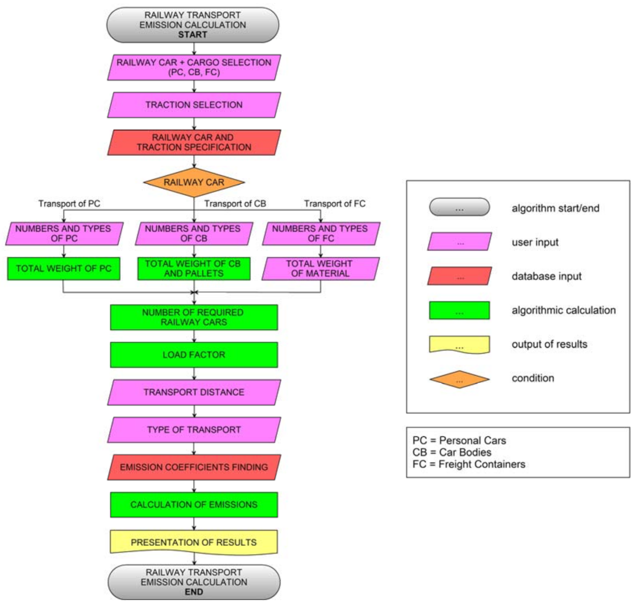
3.3. Proposal of a Customized Approach to GHG Emission Calculations in RFT for the AI

A proposal for a customized approach to the GHG emission calculations in the context of RFT for the AI is presented in Figure 2. The proposed approach is based on the conclusions obtained from the semi-structured interviews and comparative content analysis of available GHG emission calculators.

The customized approach to GHG emission calculations for RFT consists of five consecutive user steps. In the first step, the user selects a specific type of transported cargo (PC, CB, or FC) and a specific railway car (RC_1–32). In the second step, the user selects between dependent or independent traction, or can choose the ratio of dependent and independent traction. Subsequently, information about the selected railway car and information about the selected traction is retrieved from the database of railway cars. In the next steps, the GHG emission calculations are different according to the type of transported cargo (PC, CB or FC).

In the third step:

• In the case of PC transport, the user enters the number of individual types of transported PC;
• In the case of CB transport, the user enters the number of individual types of transported CB;
• In the case of FC transport, the user enters the number of individual types of transported FC and the total weight of transported material.

Subsequently, the total weight of the transported cargo is algorithmically calculated as follows:

• In the case of PC transport, as the total weight of all transported PC;
• In the case of CB transport, as the total weight of all transported CB including all transported pallet weight;
• In the case of FC transport, as the total weight of all transported FC including all transported material weight.

The required number of railway car(s) of the type specified for transport is determined from the input parameters entered by the user, information from the database and restrictive assumptions. Subsequently, the load factor for this transport is calculated for all railway car(s). In the fourth step, the user inserts the total transport distance. In the fifth step, the user decides whether it is a one-way or return transport. Subsequently, the emission coefficients for the calculated load factor are found in the emission coefficients database. Based on all inputs, GHG emissions are algorithmically calculated. Finally, the results of GHG emissions are presented according to the requirements of the company.

An overview of all the variables used is shown in alphabetical order in Appendix F. The following restrictive assumption (Equation (1)) must be taken into consideration with regard to the transported weight of the cargo:

for RC₁ to RC₃₂: V [t] ≤ (n_c [−] × V_max [t]), n_c ∈ N,

(1)

where RC_1–32 represent different types of railway cars, V is the weight of the freight, n_c is the required number of railway cars for transport, and V_max is the maximum freight weight of the railway cars required for transport.

The following universal and specific restrictive assumptions (Equation (2)) must be taken into consideration with regard to the transported volume of the cargo:

for RC₁ to RC₃₂: LV [−] ≤ (n_c [−] × LV_max [−]), n_c ∈ N,
for RC₁ to RC₂₅: LV [−] ≤ (n_c [−] × LV_max [−]), n_c ∈ N, LV_max = <10;11>,
for RC₂₆ to RC₂₉: LV [−] ≤ (n_c [−] × LV_max [−]), n_c ∈ N, LV_max = <8;10>,
for RC₃₀ to RC₃₂: LV [−] ≤ (n_c [−] × LV_max [−]), n_c ∈ N, LV_max = <1;4>,

(2)

where RC_1–32 represent different types of railway cars, LV is the load volume of the freight, n_c is the required number of railway cars for transport, and LV_max is the maximum load volume of the railway car required for transport.

The maximum load volumes of railway cars for transportation of PC and CB are defined in accordance with the following algorithmic techniques (Equation (3)):

IF transport of PC in RC_1-25 from plant A THEN LV_max = 10,
IF transport of PC in RC_1-25 from plant B THEN LV_max = 11,
IF transport of CB in RC₂₆ OR RC₂₈ THEN LV_max = 8,
IF transport of CB in RC₂₇ OR RC₂₉ THEN LV_max = 10,

(3)

where RC_1–32 represent different types of railway cars and LV_max is the maximum load volume of the railway car required for transport.

The maximum load volumes of railway cars for transportation of FC are defined in accordance with the following algorithmic techniques (Equation (4)):

IF transport of FC in RC₃₀ OR RC₃₁ THEN for FC₁: LV_max = 2,
IF transport of FC in RC₃₀ OR RC₃₁ THEN for FC₂: LV_max = 1,
IF transport of FC in RC₃₀ OR RC₃₁ THEN for FC₃: LV_max = 1,
IF transport of FC in RC₃₂ THEN for FC₁: LV_max = 4,
IF transport of FC in RC₃₂ THEN for FC₂: LV_max = 2,
IF transport of FC in RC₃₂ THEN for FC₃: LV_max = 2,

(4)

where RC_30–32 represent different types of railway cars for transportation of FC, FC_1–3 is the different types of FC, and LV_max is the maximum load volume of the railway car.

Loading of FC is possible in the following combinations only for RC₃₂ in accordance with the algorithmic techniques (Equation (5)):

IF transport of FC in RC₃₂ THEN for FC₁ = 2 AND FC₂ = 1,
IF transport of FC in RC₃₂ THEN for FC₁ = 2 AND FC₃ = 1,
IF transport of FC in RC₃₂ THEN for FC₂ = 1 AND FC₃ = 1,

(5)

where RC₃₂ represents type of railway cars for transportation of FC and FC_1–3 is the different types of FC.

The weight of the freight is determined according to Equation (6):

for PC: V = {(n_pc1 × V_PC1) + (n_pc2 × V_PC2) + … + (n_pc8 × V_PC8)} [t],
n_pck ∈ N, k ∈ <1;8>,
for CB: V = {(n_cb1 × (V_CB1 + V_P1)) + (n_cb2 × (V_CB2 + V_P2))} [t],
n_cbl ∈ N, l ∈ <1;2>,
for FC: V = {(n_fc1 × (V_FC1 + V_C1)) + (n_fc2 × (V_FC2 + V_C2)) + (n_fc3 × (V_FC3 + V_C3))} [t],
n_fcm ∈ N, m ∈ <1;3>,

(6)

where V is the weight of the freight, n_pck is the number of transported PC of type k, V_PCk is the weight of the PC of type k, k is the type of transported PC, n_cbl is the number of transported CB of type l, V_CBl is the weight of the CB of type l, V_Pl is the weight of the pallet for CB of type l, l is the type of transported CB, n_fcm is the number of transported FC of type m, V_FCm is the weight of the FC of type m, V_Cm is the weight of the freight in FC of type m, and m is the type of transported FC.

The railway car(s) load factor is calculated according to Equation (7):

LF = round up [V/(n_c × V_max)] [−], LF ∈ <0;1>, n_c ∈ N,

(7)

where LF is the railway car(s) load factor, V is the weight of the freight, n_c is the required number of railway cars for transport, and V_max is the maximum freight weight of the railway car(s) required for transport.

The appropriate emission coefficients are identified in accordance with the following algorithmic techniques (Equation (8)) with regard to the type of transport:

IF return transport THEN search emission coefficients values
for C_dWtTb, C_dWtTf, C_dTtWb, C_dTtWf, C_iWtTb, C_iWtTf, C_iTtWb and C_iTtWf,
IF one-way transport THEN search emission coefficients values
for C_dWtTb, C_dWtTf, C_dTtWb, C_dTtWf, C_iWtTb, C_iWtTf, C_iTtWb, C_iTtWf, C_d0WtTb, C_d0WtTf,
C_d0TtWb, C_d0TtWf, C_i0WtTb, C_i0WtTf, C_i0TtWb and C_i0TtWf,

(8)

where C_dWtTb is the appropriate emission coefficient of CO₂ or SO₂ of biogenic origin (hereinafter BO) calculated using the WtT approach for dependent traction, C_dWtTf is the appropriate emission coefficient of CO₂ or SO₂ of fossil origin (hereinafter FO) calculated using the WtT approach for dependent traction, C_dTtWb is the appropriate emission coefficient of CO₂ or SO₂ of BO calculated using the TtW approach for dependent traction, C_dTtWf is the appropriate emission coefficient of CO₂ or SO₂ of FO calculated using the TtW approach for dependent traction, C_iWtTb is the appropriate emission coefficient of CO₂ or SO₂ of BO calculated using the WtT approach for independent traction, C_iWtTf is the appropriate emission coefficient of CO₂ or SO₂ of FO calculated using the WtT approach for independent traction, C_iTtWb is the appropriate emission coefficient of CO₂ or SO₂ of BO calculated using the TtW approach for independent traction, C_iTtWf is the appropriate emission coefficient of CO₂ or SO₂ of FO calculated using the TtW approach for independent traction, C_d0WtTb is the appropriate emission coefficient for the empty load of CO₂ or SO₂ of BO calculated using the WtT approach for dependent traction, C_d0WtTf is the appropriate emission coefficient for the empty load of CO₂ or SO₂ of FO calculated using the WtT approach for dependent traction, C_d0TtWb is the appropriate emission coefficient for the empty load of CO₂ or SO₂ of BO calculated using the TtW approach for dependent traction, C_d0TtWf is the appropriate emission coefficient for the empty load of CO₂ or SO₂ of FO calculated using the TtW approach for dependent traction, C_i0WtTb is the appropriate emission coefficient for the empty load of CO₂ or SO₂ of BO calculated using the WtT approach for independent traction, C_i0WtTf is the appropriate emission coefficient for the empty load of CO₂ or SO₂ of FO calculated using the WtT approach for independent traction, C_i0TtWb is the appropriate emission coefficient for the empty load of CO₂ or SO₂ of BO calculated using the TtW approach for independent traction, and C_i0TtWf is the appropriate emission coefficient for the empty load of CO₂ or SO₂ of FO calculated using the TtW approach for independent traction.

Specific values of emission coefficients already include the route profile, the energy mix of the state, and the average speed of the vehicle, etc. CO₂ and SO₂ emissions are calculated for a specific shipment realized by RFT. The proposed approach is divided according to the identified requirements of the company into return transportation and one-way transportation. In the case of return transportation, Equations (9)–(22) are applied. In the case of one-way transportation, Equations (9)–(37) are applied.

The total CO₂ or SO₂ emissions produced by return transportation are calculated as Equation (9):

T [kg_CO2e/SO2e] = R [kg_CO2e/SO2e],

(9)

where T corresponds to the total CO₂ or SO₂ emissions produced by transportation and R is the total CO₂ or SO₂ emissions produced by the return transportation.

The total CO₂ or SO₂ emissions R produced by the return transportation are calculated using the WtW approach (Equation (10)):

R [kg_CO2e/SO2e] = R_WtT [kg_CO2e/SO2e] + R_TtW [kg_CO2e/SO2e],

(10)

where R_WtT is the CO₂ or SO₂ emissions calculated using the WtT approach and R_TtW is the CO₂ or SO₂ emissions calculated using the TtW approach.

R_WtT is the CO₂ or SO₂ emissions calculated using the WtT approach consisting of two parts (Equation (11)):

R_WtT [kg_CO2e/SO2e] = R_WtTb [kg_CO2e/SO2e] + R_WtTf [kg_CO2e/SO2e],

(11)

where R_WtTb is the CO₂ or SO₂ emissions of BO calculated using the WtT approach and R_WtTf is the CO₂ or SO₂ emissions of FO calculated using the WtT approach.

R_TtW is the CO₂ or SO₂ emissions calculated using the TtW approach consisting of two parts (Equation (12)):

R_TtW [kg_CO2e/SO2e] = R_TtWb [kg_CO2e/SO2e] + R_TtWf [kg_CO2e/SO2e],

(12)

where R_TtWb is the CO₂ or SO₂ emissions of BO calculated using the TtW approach and R_TtWf is the CO₂ or SO₂ emissions of FO calculated using the TtW approach.

The CO₂ or SO₂ emissions of BO calculated using the WtT approach R_WtTb are calculated according to Equation (13):

R_WtTb [kg_CO2e/SO2e] = {S_d1 [−] × C_dWtTb [kg_CO2e/SO2e/tkm]
+ S_i1 [−] × C_iWtTb [kg_CO2e/SO2e/tkm]} × V [t] × L₁ [km],

(13)

where S_d1 is the share of the total length of transport realized by RFT using dependent traction, C_dWtTb is the appropriate emission coefficient of CO₂ or SO₂ of BO calculated using the WtT approach for dependent traction, S_i1 is the share of the total length of transport realized by RFT using independent traction, C_iWtTb is the appropriate emission coefficient of CO₂ or SO₂ of BO calculated using the WtT approach for independent traction, V is the weight of the freight, and L₁ is the total transport distance.

The CO₂ or SO₂ emissions of FO calculated using the WtT approach R_WtTf are calculated according to Equation (14):

R_WtTf [kg_CO2e/SO2e] = {S_d1 [−] × C_dWtTf [kg_CO2e/SO2e/tkm]
+ S_i1 [−] × C_iWtTf [kg_CO2e/SO2e/tkm]} × V [t] × L₁ [km],

(14)

where S_d1 is the share of the total length of transport realized by RFT using dependent traction, C_dWtTf is the appropriate emission coefficient of CO₂ or SO₂ of FO calculated using the WtT approach for dependent traction, S_i1 is the share of the total length of transport realized by RFT using independent traction, C_iWtTf is the appropriate emission coefficient of CO₂ or SO₂ of FO calculated using the WtT approach for independent traction, V is the weight of the freight, and L₁ is the total transport distance.

The CO₂ or SO₂ emissions of BO calculated using the TtW approach R_TtWb are calculated according to Equation (15):

R_TtWb [kg_CO2e/SO2e] = {S_d1 [−] × C_dTtWb [kg_CO2e/SO2e/tkm]
+ S_i1 [−] × C_iTtWb [kg_CO2e/SO2e/tkm]} × V [t] × L₁ [km],

(15)

where S_d1 is the share of the total length of transport realized by RFT using dependent traction, C_dTtWb is the appropriate emission coefficient of CO₂ or SO₂ of BO calculated using the TtW approach for dependent traction, S_i1 is the share of the total length of transport realized by RFT using independent traction, C_iTtWb is the appropriate emission coefficient of CO₂ or SO₂ of BO calculated using the TtW approach for independent traction, V is the weight of the freight, and L₁ is the total transport distance.

The CO₂ or SO₂ emissions of FO calculated using the TtW approach R_TtWf are calculated according to Equation (16):

R_TtWf [kg_CO2e/SO2e] = {S_d1 [−] × C_dTtWf [kg_CO2e/SO2e/tkm]
+ S_i1 [−] × C_iTtWf [kg_CO2e/SO2e/tkm]} × V [t] × L₁ [km],

(16)

where S_d1 is the share of the total length of transport realized by RFT using dependent traction, C_dTtWf is the appropriate emission coefficient of CO₂ or SO₂ of FO calculated using the TtW approach for dependent traction, S_i1 is the share of the total length of transport realized by RFT using independent traction, C_iTtWf is the appropriate emission coefficient of CO₂ or SO₂ of FO calculated using the TtW approach for independent traction, V is the weight of the freight, and L₁ is the total transport distance.

The share of the total length of transport realized by RFT using dependent traction S_d1 is calculated according to Equation (17):

S_d1 [−] = L_1d [km]/L₁ [km], L_1d ≤ L₁, S_d1 ∈ <0;1>,

(17)

where L_1d is the length of transport realized by RFT using dependent traction and L₁ is the total transport distance.

The share of the total length of transport realized by RFT using independent traction S_i1 is calculated according to Equation (18):

S_i1 [−] = L_1i [km]/L₁ [km], L_1i ≤ L₁, S_i1 ∈ <0;1>,

(18)

where L_1i is the length of transport realized by RFT using independent traction and L₁ is the total transport distance.

The following (Equation (19)) must always apply to variables from Equations (17) and (18):

S_d1 [−] + S_i1 [−] = 1, {S_d1, S_i1} ∈ <0;1>,
L_1d [km] + L_1i [km] = L₁ [km],

(19)

where S_d1 is the share of the total length of transport realized by RFT using dependent traction, S_i1 is the share of the total length of transport realized by RFT using independent traction, L_1d is the length of transport realized by RFT using dependent traction, L_1i is the length of transport realized by RFT using independent traction, and L₁ is the total transport distance.

If the transport is carried out exclusively with the use of dependent traction, the following applies (Equation (20)):

S_d1 [−] = 1,
S_i1 [−] = 0,

(20)

where S_d1 is the share of the total length of transport realized by RFT using dependent traction and S_i1 is the share of the total length of transport realized by RFT using independent traction.

If the transport is carried out exclusively with the use of independent traction, the following applies (Equation (21)):

S_d1 [−] = 0,
S_i1 [−] = 1,

(21)

where S_d1 is the share of the total length of transport realized by RFT using dependent traction and S_i1 is the share of the total length of transport realized by RFT using independent traction.

If the transport is carried out with the use of dependent and independent traction, the following applies (Equation (22)):

S_d1 [−] + S_i1 [−] = 1,

(22)

where S_d1 is the share of the total length of transport realized by RFT using dependent traction and S_i1 is the share of the total length of transport realized by RFT using independent traction.

The total CO₂ or SO₂ emissions produced by one-way transportation are calculated as Equation (23):

T [kg_CO2e/SO2e] = R [kg_CO2e/SO2e] + O [kg_CO2e/SO2e],

(23)

where T corresponds to the total CO₂ or SO₂ emissions produced by transportation, R is the total CO₂ or SO₂ emissions produced by the return transportation, and O is the additional CO₂ or SO₂ emissions (the penalty for an unloaded railway cars).

The additional CO₂ or SO₂ emissions (the penalty for an unloaded railway cars) O are calculated using the WtW approach (Equation (24)):

O [kg_CO2e/SO2e] = O_WtT [kg_CO2e/SO2e] + O_TtW [kg_CO2e/SO2e],

(24)

where O_WtT is the CO₂ or SO₂ emissions calculated using the WtT approach and O_TtW is the CO₂ or SO₂ emissions calculated using the TtW approach.

O_WtT is the CO₂ or SO₂ emissions calculated using the WtT approach consisting of two parts (Equation (25)):

O_WtT [kg_CO2e/SO2e] = O_WtTb [kg_CO2e/SO2e] + O_WtTf [kg_CO2e/SO2e],

(25)

where O_WtTb is the CO₂ or SO₂ emissions of BO calculated using the WtT approach and O_WtTf is the CO₂ or SO₂ emissions of FO calculated using the WtT approach.

O_TtW is the CO₂ or SO₂ emissions calculated using the TtW approach consisting of two parts (Equation (26)):

O_TtW [kg_CO2e/SO2e] = O_TtWb [kg_CO2e/SO2e] + O_TtWf [kg_CO2e/SO2e],

(26)

where O_TtWb is the CO₂ or SO₂ emissions of BO calculated using the TtW approach and O_TtWf is the CO₂ or SO₂ emissions of FO calculated using the TtW approach.

The additional transport distance L₂ as a penalty for unloaded railway cars is calculated according to Equation (27):

L₂ [km] = L₁ [km] × l [−],

(27)

where L₁ is the transport distance and l is the internal coefficient defined by the company.

The CO₂ or SO₂ emissions of BO calculated using the TtW approach O_WtTb are calculated according to Equation (28):

O_WtTb [kg_CO2e/SO2e] = {S_d2 [−] × C_d0WtTb [kg_CO2e/SO2e/tkm]
+ S_i2 [−] × C_i0WtTb [kg_CO2e/SO2e/tkm]} × V [t] × L₂ [km],

(28)

where S_d2 is the share of the additional length of transport realized by RFT using dependent traction, C_d0WtTb is the appropriate emission coefficient for the empty load of CO₂ or SO₂ of BO calculated using the WtT approach for dependent traction, S_i2 is the share of the additional length of transport realized by RFT using independent traction, C_i0WtTb is the appropriate emission coefficient for the empty load of CO₂ or SO₂ of BO calculated using the WtT approach for independent traction, V is the weight of the load, and L₂ is the additional transport distance.

The CO₂ or SO₂ emissions of FO calculated using the WtT approach O_WtTf are calculated according to Equation (29):

O_WtTf [kg_CO2e/SO2e] = {S_d2 [−] × C_d0WtTf [kg_CO2e/SO2e/tkm]
+ S_i2 [−] × C_i0WtTf [kg_CO2e/SO2e/tkm]} × V [t] × L₂ [km],

(29)

where S_d2 is the share of the additional length of transport realized by RFT using dependent traction, C_d0WtTf is the appropriate emission coefficient for the empty load of CO₂ or SO₂ of FO calculated using the WtT approach for dependent traction, S_i2 is the share of the additional length of transport realized by RFT using independent traction, C_i0WtTf is the appropriate emission coefficient for the empty load of CO₂ or SO₂ of FO calculated using the WtT approach for independent traction, V is the weight of the freight, and L₂ is the additional transport distance.

The CO₂ or SO₂ emissions of BO calculated using the WtT approach O_TtWb are calculated according to Equation (30):

O_TtWb [kg_CO2e/SO2e] = {S_d2 [−] × C_d0TtWb [kg_CO2e/SO2e/tkm]
+ S_i2 [−] × C_i0TtWb [kg_CO2e/SO2e/tkm]} × V [t] × L₂ [km],

(30)

where S_d2 is the share of the additional length of transport realized by RFT using dependent traction, C_d0TtWb is the appropriate emission coefficient for the empty load of CO₂ or SO₂ of BO calculated using the TtW approach for dependent traction, S_i2 is the share of the additional length of transport realized by RFT using independent traction, C_i0TtWb is the appropriate emission coefficient for the empty load of CO₂ or SO₂ of BO calculated using the TtW approach for independent traction, V is the weight of the freight, and L₂ is the additional transport distance.

The CO₂ or SO₂ emissions of FO calculated using the TtW approach O_TtWf are calculated according to Equation (31):

O_TtWf [kg_CO2e/SO2e] = {S_d2 [−] × C_d0TtWf [kg_CO2e/SO2e/tkm]
+ S_i2 [−] × C_i0TtWf [kg_CO2e/SO2e/tkm]} × V [t] × L₂ [km],

(31)

where S_d2 is the share of the additional length of transport realized by RFT using dependent traction, C_d0TtWf is the appropriate emission coefficient for the empty load of CO₂ or SO₂ of FO calculated using the TtW approach for dependent traction, S_i2 is the share of the additional length of transport realized by RFT using independent traction, C_i0TtWf is the appropriate emission coefficient for the empty load of CO₂ or SO₂ of FO calculated using the TtW approach for independent traction, V is the weight of the freight, and L₂ is the additional transport distance.

The share of the additional length of transport realized by RFT using dependent traction S_d2 is calculated according to Equation (32):

S_d2 [−] = L_2d [km]/L₂ [km], L_2d ≤ L₂, S_d2 ∈ <0;1>,

(32)

where L_2d is the additional length of transport realized by RFT using dependent traction and L₂ is the additional transport distance.

The share of the additional length of transport realized by RFT using independent traction S_i2 is calculated according to Equation (33):

S_i2 [−] = L_2i [km]/L₂ [km], L_2i ≤ L₂, S_i2 ∈ <0;1>,

(33)

where L_2i is the additional length of transport realized by RFT using independent traction and L₂ is the additional transport distance.

The following (Equation (34)) must always apply to variables from Equations (32) and (33):

S_d2 [−] + S_i2 [−] = 1, {S_d2, S_i2} ∈ <0;1>,
L_2d [km] + L_2i [km] = L₂ [km],

(34)

where S_d2 is the share of the additional length of transport realized by RFT using dependent traction, S_i2 is the share of the additional length of transport realized by RFT using independent traction, L_2d is the additional length of transport realized by RFT using dependent traction, L_2i is the additional length of transport realized by RFT using independent traction, and L₂ is the additional transport distance.

If the transport is carried out exclusively with the use of dependent traction, the following applies (Equation (35)):

S_d2 [−] = 1,
S_i2 [−] = 0,

(35)

where S_d2 is the share of the additional length of transport realized by RFT using dependent traction and S_i2 is the share of the additional length of transport realized by RFT using independent traction.

If the transport is carried out exclusively with the use of independent traction, the following applies (Equation (36)):

S_d2 [−] = 0,
S_i2 [−] = 1,

(36)

where S_d2 is the share of the additional length of transport realized by RFT using dependent traction and S_i2 is the share of the additional length of transport realized by RFT using independent traction.

If the transport is carried out with the use of dependent and independent traction, the following applies (Equation (37)):

S_d2 [−] + S_i2 [−] = 1,

(37)

where S_d2 is the share of the additional length of transport realized by RFT using dependent traction and S_i2 is the share of the additional length of transport realized by RFT using independent traction.

In the following Section 3.4, the proposed customized approach to GHG emission calculations in RFT for the AI will be applied and verified in the form of an interpretative case study, theoretically described in Section 2.3.

3.4. Case Study Assumptions and Calculations

The proposed customized approach to GHG emission calculations in RFT for the AI is applied and verified in the form of the interpretative case study. This case study was conducted in a company, which is the leader of the AI operating on the Czech Republic market. The proposed approach was tested for real transport requirement with these parameters:

• Type of cargo: FC;
• Railway car: RC₃₂ (Sggns S183);
• Traction: 62% dependent traction (S_d1 = 0.62), 38% independent traction (S_i1 = 0.38);
• Numbers and types of FC: 24 FC₂;
• Weight of the freight in one FC₂ (V_C2): 27.25 t;
• Total transport distance (L₁): 472 km;
• Length of transport realized by RFT using dependent traction (L_1d): 292.64 km;
• Length of transport realized by RFT using independent traction (L_1i): 179.36 km;
• Type of transport: return.

The maximum load volume of railway car RC₃₂ for transportation of FC₂ is defined (according to Equation (4)) as follows (Equation (38)):

IF transport of FC in RC₃₂ THEN for FC₂: LV_max = 2,

(38)

where RC₃₂ represents type of railway car for transportation of FC, FC₂ is the type of FC, and LV_max is the maximum load volume of the railway car RC₃₂.

Due to the fact, that 24 FC_2′s are transported and the LV_max of FC₂ is 2 (according to Equation (4)), it will be necessary to use 12 RC₃₂’s for this transport (n_c = 12).

The weight of the freight is determined as follows (Equation (39) according to Equation (6)):

for FC: V = {(0 × (2.2 + 0)) + (24 × (3.8 + 27.25)) + (0 × (3.9 + 0))} [t],
for FC: V = {(0 + 745.2 + 0)} [t],
for FC: V = 745.2 [t],

(39)

where V is the weight of the freight.

The following restrictive assumption (Equation (40)) must be taken into consideration with regards to the transported weight of the cargo (according to Equation (1)):

for RC₃₂: 745.2 [t] ≤ (12 [−] × 67.5 [t]),
for RC₃₂: 745.2 [t] ≤ 810.0 [t],

(40)

where RC₃₂ represents type of railway car, V is the weight of the freight, n_c is the required number of railway cars for transport, and V_max is the maximum freight weight of the railway cars required for transport. The restrictive assumption (according to Equation (1)) is met.

The following specific restrictive assumption (Equation (41)) must be taken into consideration with regards to the transported volume of the cargo (according to Equation (2)):

for RC32: 24 [−] ≤ (12 [−] × 2 [−]),
for RC32: 24 [−] ≤ 24 [−],

(41)

where RC₃₂ represents type of the railway car, LV is the load volume of the freight, n_c is the required number of railway cars for transport, and LV_max is the maximum load volume of the railway car required for transport. The restrictive assumption (according to Equation (2)) is met.

The railway car load factor is calculated as follows (Equation (42) according to Equation (7)):

LF = round up [745.2/(12 × 67.5)] [−],
LF = 0.92 [−],

(42)

where LF is the railway car load factor.

The appropriate CO₂ emission coefficients for return transport and LF = 0.92 (according to Equation (7)) are searched in the database of GHG emission coefficients (according to Equation (8)) [79]:

• C_dWtTb = 0.001802327 [kg_CO2e/tkm];
• C_dWtTf = 0.009762854 [kg_CO2e/tkm];
• C_dTtWb = 0.000000000 [kg_CO2e/tkm];
• C_dTtWf = 0.000000000 [kg_CO2e/tkm];
• C_iWtTb = 0.000109177 [kg_CO2e/tkm];
• C_iWtTf = 0.002784794 [kg_CO2e/tkm];
• C_iTtWb =0.001200000 [kg_CO2e/tkm];
• C_iTtWf = 0.015700000 [kg_CO2e/tkm].

The total CO₂ emissions produced by return transportation are calculated as Equation (43) (according to Equation (9)):

T = 5167.724435009 [kg_CO2e],

(43)

where T represents the total CO₂ emissions produced by transportation.

The total CO₂ emissions R produced by the return transportation are calculated using the WtW approach as Equation (44) (according to Equation (10)):

R = 2908.886118209 + 2258.838316800 [kg_CO2e].

(44)

R_WtT is the CO₂ emissions calculated using the WtT approach consisting of two parts (Equation (45) according to Equation (11)):

R_WtT = 407.635548192 + 2501.250570017 [kg_CO2e].

(45)

R_TtW is the CO₂ emissions calculated using the TtW approach consisting of two parts (Equation (46) according to Equation (12)):

R_TtW = 160.390886400 + 2098.447430400 [kg_CO2e].

(46)

The CO₂ emissions of BO calculated using the WtT approach R_WtTb are calculated as Equation (47) (according to Equation (13)):

R_WtTb [kg_CO2e] = {0.62 [−] × 0.001802327 [kg_CO2e/tkm]
+ 0.38 [−] × 0.000109177 [kg_CO2e/tkm]} × 745.2 [t] × 472 [km],
R_WtTb [kg_CO2e] = 407.635548192.

(47)

The CO₂ emissions of FO calculated using the WtT approach R_WtTf are calculated as Equation (48) (according to Equation (14)):

R_WtTf [kg_CO2e] = {0.62 [−] × 0.009762854 [kg_CO2e/tkm]
+ 0.38 [−] × 0.002784794 [kg_CO2e/tkm]} × 745.2 [t] × 472 [km],
R_WtTf [kg_CO2e] = 2501.250570017.

(48)

The CO₂ emissions of BO calculated using the TtW approach R_TtWb are calculated as Equation (49) (according to Equation (15)):

R_TtWb [kg_CO2e] = {0.62 [−] × 0.000000000 [kg_CO2e/tkm]
+ 0.38 [−] × 0.001200000 [kg_CO2e/tkm]} × 745.2 [t] × 472 [km],
R_TtWb [kg_CO2e] = 160.390886400.

(49)

The CO₂ emissions of FO calculated using the TtW approach R_TtWf are calculated as Equation (50) (according to Equation (16)):

R_TtWf [kg_CO2e] = {0.62 [−] × 0.000000000 [kg_CO2e/tkm]
+ 0.38 [−] × 0.015700000 [kg_CO2e/tkm]} × 745.2 [t] × 472 [km],
R_TtWf [kg_CO2e] = 2098.447430400.

(50)

Finally, the resulting GHG emissions are presented according to the requirements of the company as total GHG emissions, average GHG emissions per 1 km, average GHG emissions per 1 t, and average GHG emissions per 1 tkm (Table 2, Section 4).

The same procedure as in Equations (43)–(50) can be used to calculate SO₂ GHG emissions. The proposed customized approach was also tested except with FC transport instead of PC and CB transport, but due to the range of the manuscript, the individual calculations are not listed here. The proposed customized approach to GHG emission calculations in RFT for the AI (Section 3.3) has been applied and verified.

4. Results and Discussion

The aim of this article was to propose a fully customized approach to GHG emission calculations in RFT for the AI. Firstly, the requirements for the calculation of GHG emissions from RFT in the AI were identified using three-round semi-structured interviews with highly qualified and well-founded employees of a leading company in the AI operating on the Czech Republic market. As a result, it was found that the area of GHG emission calculations is essential for the company because the company strives to minimize negative logistic impacts on the environment and society. The company does not currently use any RFT emission calculators or other similar tools, as there is no suitable calculator available to meet company requirements or restrictive assumptions. Following this, available railway freight GHG emission calculators were identified and analyzed from the perspective of suitability for the AI using comparative content analysis. As a result, we can state that none of the analyzed GHG emission calculators in the field of RFT is suitable for the needs of GHG emission calculations in the AI because it does not meet all the identified assumptions based on the results of the three-round semi-structured interview. Finally, a fully customized approach to GHG emission calculations in RFT for the AI was proposed, applied, and verified in the form of an interpretative case study. The summary of results for the test calculation is presented in

Table 2. Summary of results for test calculations [authors].

CO2 Emissions	WtT Biogenic Origin [kgCO2e]	WtT Fossil Origin [kgCO2e]	TtW Biogenic Origin [kgCO2e]	TtW Fossil Origin [kgCO2e]
Total by origin	407.635548192	2501.250570017	160.390886400	2098.447430400
Average per 1 km	0.863634636	5.299259682	0.339811200	4.445863200
Average per 1 t	0.547014960	3.356482246	0.215232000	2.815952000
Average per 1 tkm	0.001158930	0.007111191	0.000456000	0.005966000
Total WtT	2908.886118209		NC
Total TtW	NC		2258.838316800
Total WtW	5167.724435009

Notes: CO_2e—carbon dioxide equivalent, WtT—Well-to-Tank approach, TtW—Tank-to-Wheel approach, WtW—Well-to-Wheel approach, NC—not calculable.

.

The CO₂ emissions are presented in Table 2, according to the requirements of the company, as total GHG emissions, average GHG emissions per 1 km, average GHG emissions per 1 t, and average GHG emissions per 1 ton-kilometer. At the same time, the presented results are divided into emissions by origin (BO and FO) and by approach (WtT, TtW, and WtW approach). The total CO₂ emissions of the test calculation calculated by the WtW approach are 5167.72 kg_CO2e. These CO₂ emissions consist of emissions calculated by the WtT approach (2908.88 kg_CO2e) and TtW approach (2258.83 kg_CO2e). The overall results of the model calculation were compared with the results of the EcoTransIT emission calculator [71] and can be considered valid. If the input parameters change, the results also change in a reasonable manner.

This proposed fully customized approach to GHG emission calculations in RFT can be used by all companies in the AI worldwide, because the company that was used in the interpretive case study has plants around the world and the proposed approach was also tested for shipments in individual plants.

This study contains some limitations that are worth discussing. The first limitation is the processed theoretical background. The authors cannot guarantee the use of all available sources, but the processed theoretical background contains all the essential knowledge in the field and the basic axioms. At the same time, the existence of other available materials that were not used in the processed theoretical background cannot be ruled out. Another limitation is the area of identification of assumptions for the GHG emission calculations from RFT. These assumptions were identified and synthetized by using three-round semi-structured interviews. It cannot be completely ruled out that there may be a company in the AI that will have a specific requirement for GHG emission calculations that is not implemented in the proposed approach. On the other side, semi-structured interviews were conducted with highly qualified and well-founded employees of a company which is the leader in the AI Czech Republic market. These employees have sufficient experience across the entire AI to be able to define all requirements for GHG emission calculations. The last potential limitation may lie in the selection of available GHG emission calculators for analysis. Again, the existence of other GHG emission calculators than those analyzed cannot be ruled out. In any case, analyzed GHG emission calculators were selected in a clear, scientific, and objective procedure.

5. Conclusions

The issue of global warming and related GHG emissions are a current topic from not only a scientific but also a practical perspective. This is an area of interest to many stakeholders, such as residents, employees, politicians, activists, shareholders, company leaders, state control bodies, state administrations, and local self-governments. From the point of view of the Czech Republic, the AI has an ambivalent character. On the one hand, it is a significant driver of the Czech economy. However, on the other hand, due to large supply chains, it negatively affects the environment and human society as a whole. Automotive companies are constantly striving to reduce negative environmental and social impacts, but appropriate tools must be in place. None of the analyzed GHG emission calculators in the field of RFT is suitable for the needs of GHG emission calculations in the AI because they does not meet all the identified conditions and requirements based on the results of the three-round semi-structured interview. A fully customized approach to GHG emission calculations in RFT for the AI was proposed, tested, and validated. We assume that the proposed approach can be transformed into a software tool (software emission calculator fully customized for the AI) which will be used to support logistic planning and decision making. The possible extension of this research may focus on the proposal of a framework for GHG emission calculations in multimodal transport. Another option is to specialize in RFT in the context of GHG emission calculations in another very specific sector, such as the chemical industry.

References

1. Rungskunroch, P.; Shen, Z.J.; Kaewunruen, S. Benchmarking environmental and economic impacts from the HSR networks considering life cycle perspectives. Environ. Impact Assess. Rev. 2021, 90, 106608. [Google Scholar] [CrossRef]
2. Cichozs, M.; Pluta-Zaremba, A. How to improve freight transport emissions’ management? LogForum 2019, 15, 93–105. [Google Scholar] [CrossRef]
3. Lee, D.; Balachandran, S.; Pachon, J.; Shankaran, R.; Lee, S.; Mulholland, J.A.; Russell, A.G. Ensemble-trained PM2.5 source apportionment approach for health studies. Environ. Sci. Technol. 2009, 43, 7023–7031. [Google Scholar] [CrossRef] [PubMed]
4. Wang, W.W.; Zhang, M.; Zhou, M. Using LMDI method to analyze transport sector CO2 emissions in China. Energy 2011, 10, 5909–5915. [Google Scholar] [CrossRef]
5. Lee, S.; Wang, Y.H.; Russell, A.G. Assessment of secondary organic carbon in the southeastern United States: A review. J. Air Waste Manag. Assoc. 2010, 60, 1282–1292. [Google Scholar] [CrossRef] [PubMed] [Green Version]
6. Lee, S.; Russell, A.G.; Baumann, K. Source apportionment of fine particulate matter in the southeastern united states. J. Air Waste Manag. Assoc. 2007, 57, 1123–1135. [Google Scholar] [CrossRef] [Green Version]
7. Lee, S.; Liu, W.; Wang, Y.H.; Russell, A.G.; Edgerton, E.S. Source apportionment of PM2.5: Comparing PMF and CMB results for four ambient monitoriniz sites in the southeastern United States. Atmos. Environ. 2008, 42, 4126–4137. [Google Scholar] [CrossRef]
8. Rungskunroch, P.; Shen, Z.J.; Kaewunruen, S. Getting it right on the policy prioritization for rail decarbonization: Evidence from whole-life CO2e emissions of railway systems. Front. Built Environ. 2021, 7, 638507. [Google Scholar] [CrossRef]
9. Jung, J.; Lyu, Y.; Lee, M.; Hwang, T.; Lee, S.; Oh, S. Impact of Siberian forest fires on the atmosphere over the Korean Peninsula during summer 2014. Atmos. Chem. Phys. 2016, 16, 6757–6770. [Google Scholar] [CrossRef] [Green Version]
10. Lee, S.; Baumann, K.; Schauer, J.J.; Sheesley, R.J.; Naeher, L.P.; Meinardi, S.; Blake, D.R.; Edgerton, E.S.; Russell, A.G.; Clements, M. Gaseous and particulate emissions from prescribed burning in Georgia. Environ. Sci. Technol. 2005, 39, 9049–9056. [Google Scholar] [CrossRef]
11. Jung, J.; Lee, S.; Kim, H.; Kim, D.; Lee, H.; Oh, S. Quantitative determination of the biomass-burning contribution to atmospheric carbonaceous aerosols in Daejeon, Korea, during the rice-harvest period. Atmos. Environ. 2014, 89, 642–650. [Google Scholar] [CrossRef]
12. Balachandran, S.; Pachon, J.E.; Lee, S.; Oakes, M.M.; Rastogi, N.; Shi, W.Y.; Tagaris, E.; Yan, B.; Davis, A.; Zhang, X.L.; et al. Particulate and gas sampling of prescribed fires in South Georgia, USA. Atmos. Environ. 2013, 81, 125–135. [Google Scholar] [CrossRef]
13. Liu, L.; Wang, K.; Wang, S.S.; Zhang, R.Q.; Tang, X.Y. Assessing energy consumption, CO2 and pollutant emissions and health benefits from China’s transport sector through 2050. Energy Policy 2018, 116, 382–396. [Google Scholar] [CrossRef]
14. Georgatzi, V.V.; Stamboulis, Y.; Vetsikas, A. Examining the determinants of CO2 emissions caused by the transport sector: Empirical evidence from 12 European countries. Econ. Anal. Policy 2020, 65, 11–20. [Google Scholar] [CrossRef]
15. Saboori, B.; Sapri, M.; Bin Baba, M. Economic growth, energy consumption and CO2 emissions in OECD (Organization for Economic Co-operation and Development)’s transport sector: A fully modified bi-directional relationship approach. Energy 2014, 66, 150–161. [Google Scholar] [CrossRef]
16. Hao, H.; Geng, Y.; Li, W.; Bin, G. Energy consumption and GHG emissions from China’s freight transport sector: Scenarios through 2050. Energy Policy 2015, 85, 94–101. [Google Scholar] [CrossRef]
17. Li, Y.; Du, Q.; Lu, X.R.; Wu, J.; Han, X. Relationship between the development and CO2 emissions of transport sector in China. Transp. Res. Part D Transp. Environ. 2019, 74, 1–14. [Google Scholar] [CrossRef]
18. AutoSAP. Available online: https://autosap.cz/zakladni-prehledy-automotive/obecne-zakladni-prehledy (accessed on 20 May 2021).
19. Inkinen, T.; Hämäläinen, E. Reviewing truck logistics: Solutions for achieving low emission road freight transport. Sustainability 2020, 12, 6714. [Google Scholar] [CrossRef]
20. Matusiewicz, M. Towards sustainable urban logistics: Creating sustainable urban freight transport on the example of a limited accessibility zone in Gdansk. Sustainability 2019, 11, 3879. [Google Scholar] [CrossRef] [Green Version]
21. EU Climate Action and the European Green Deal. EU Climate Action. Available online: https://ec.europa.eu/clima/policies/eu-climate-action_en (accessed on 21 May 2021).
22. Nikas, A.; Elia, A.; Boitier, B.; Koasidis, K.; Doukas, H.; Cassetti, G.; Anger-Kraavi, A.; Bui, H.; Campagnolo, L.; Miglio, R.D.; et al. Where is the EU headed given its current climate policy? A stakeholder-driven model inter-comparison. Sci. Total Environ. 2021, 793, 148549. [Google Scholar] [CrossRef]
23. Egli, F.; Stunzi, A. A dynamic climate finance allocation mechanism reflecting the Paris Agreement. Environ. Res. Lett. 2019, 14, 114024. [Google Scholar] [CrossRef]
24. Chen, S.; Wu, J.; Zong, Y. The impact of the freight transport modal shift policy on China’s carbon emissions reduction. Sustainability 2020, 12, 583. [Google Scholar] [CrossRef] [Green Version]
25. Wang, L.; Xue, X.; Zhao, Z.; Wang, Y.; Zeng, Z. Finding the de-carbonization potentials in the transport sector: Application of scenario analysis with a hybrid prediction model. Environ. Sci. Pollut. Res. 2020, 27, 21762–21776. [Google Scholar] [CrossRef] [PubMed]
26. Feng, F.; Liu, C.; Liu, H.; Ji, Z. Research on price of railway freight based on low-carbon economy. Math. Probl. Eng. 2016, 1–7. [Google Scholar] [CrossRef]
27. Kaewunruen, S.; Rungskunroch, P.; Jennings, D. A through-life evaluation of end-of-life rolling stocks considering asset recycling, energy recovering, and financial benefit. J. Clean. Prod. 2019, 212, 1008–1024. [Google Scholar] [CrossRef]
28. Krezo, S.; Mirza, O.; He, Y.P.; Makim, P.; Kaewunruen, S. Field investigation and parametric study of greenhouse gas emissions from railway plain-line renewals. Transp. Res. Part D Transp. Environ. 2016, 42, 77–90. [Google Scholar] [CrossRef]
29. Krezo, S.; Mirza, O.; Kaewunruen, S.; Sussman, J.M. Evaluation of CO2 emissions from railway resurfacing maintenance activities. Transp. Res. Part D Transp. Environ. 2018, 65, 458–465. [Google Scholar] [CrossRef]
30. Kaewunruen, S.; Sresakoolchai, J.; Yu, S.A. Global warming potentials due to railway tunnel construction and maintenance. Appl. Sci. 2020, 10, 6459. [Google Scholar] [CrossRef]
31. Petro, F.; Konečný, V. Calculation of emissions from transport services and their use for the internalisation of external costs in road transport. Procedia Eng. 2017, 192, 677–682. [Google Scholar] [CrossRef]
32. Eriksson, L.; Nielsen, L. Modelling and Control of Engines and Drivelines; John Wiley and Sons: Chennai, India, 2014. [Google Scholar]
33. Skrúcaný, T.; Kendra, M.; Kalina, T.; Jurkovič, M. Environmental comparison of different transport modes. Naše More 2018, 65, 192–196. [Google Scholar] [CrossRef]
34. Kaewunruen, S.; Sresakoolchai, J.; Peng, J.Y. Life cycle cost, energy and carbon assessments of Beijing-Shanghai high-speed railway. Sustainability 2020, 12, 206. [Google Scholar] [CrossRef] [Green Version]
35. Kaewunruen, S.; Peng, J.Y.; Phil-Ebosie, O. Digital twin aided sustainability and vulnerability audit for subway stations. Sustainability 2020, 12, 7873. [Google Scholar] [CrossRef]
36. Pan, S.; Ballot, E.; Fontane, F. The reduction of greenhouse gas emissions from freight transport by pooling supply chains. Int. J. Prod. Econ. 2013, 143, 86–94. [Google Scholar] [CrossRef]
37. Rouquet, A.; Vauché, L. A typology of logistics pooling in supply chains. Supply Chain Forum Int. J. 2015, 16, 2–12. [Google Scholar] [CrossRef]
38. Senkel, M.-P.; Durand, B.; Vo, T.l.H. La mutualisation logistique: Entre théories et pratiques. Logistique Manag. 2013, 21, 19–30. [Google Scholar] [CrossRef]
39. Lee, S.; Choi, Y.; Woo, J.; Kang, W.; Jung, J. Estimating and comparing greenhouse gas emissions with their uncertainties using different methods: A case study for an energy supply utility. J. Air Waste Manag. Assoc. 2014, 64, 1164–1173. [Google Scholar] [CrossRef] [Green Version]
40. Padgett, J.P.; Steinemann, A.C.; Clarke, J.H.; Vandenbergh, M.P. A comparison of carbon calculators. Environ. Impact Assess. Rev. 2008, 28, 106–115. [Google Scholar] [CrossRef]
41. Weigel, B.A.; Southworth, F.; Meyer, M.D. Calculators to estimate greenhouse gas emissions from public transit vehicles. Transp. Res. Rec. 2010, 2143, 125–133. [Google Scholar] [CrossRef]
42. Rabionet, S.E. How I learned to design and conduct semi-structured interviews: An ongoing and continuous journey. Qual. Rep. 2009, 35, 203–206. [Google Scholar]
43. Crist, K.; Bolling, K.; Schipperijn, J.; Hurst, S.; Takemoto, M.; Sallis, J.F.; Badland, H.; Kerr, J. Collaboration between physical activity researchers and transport planners: A qualitative study of attitudes to data driven approaches. J. Transp. Health 2018, 8, 157–168. [Google Scholar] [CrossRef]
44. Hilgarter, K.; Granig, P. Public perception of autonomous vehicles: A qualitative study based on interviews after riding an autonomous shuttle. Transp. Res. Part F Traffic Psychol. Behav. 2020, 72, 226–243. [Google Scholar] [CrossRef]
45. Qu, S.Q.; Dumay, J. The qualitative research interview. Qual. Res. Account. Manag. 2011, 8, 238–264. [Google Scholar] [CrossRef]
46. Aljohani, K.; Thompson, R.G. An examination of last mile delivery practices of freight carriers servicing business receivers in inner-city areas. Sustainability 2020, 12, 2837. [Google Scholar] [CrossRef] [Green Version]
47. Karolemeas, C.; Tsigdinos, S.; Tzouras, P.G.; Nikitas, A.; Bakogiannis, E. Determining electric vehicle charging station location suitability: A qualitative study of greek stakeholders employing thematic analysis and analytical hierarchy process. Sustainability 2021, 13, 2298. [Google Scholar] [CrossRef]
48. Kaupa, F.; Naude, M.J. Critical success factors in the supply chain management of essential medicines in the public health-care system in Malawi. J. Glob. Oper. Strat. Sour. 2021, 1, 4. [Google Scholar] [CrossRef]
49. Schlegel, A.; Birkel, H.S.; Hartmann, E. Enabling integrated business planning through big data analytics: A case study on sales and operations planning. Int. J. Phys. Distr. Logist. Manag. 2020, 11, 156. [Google Scholar] [CrossRef]
50. Mayring, P. Qualitative Content Analysis: Theoretical Foundation, Basic Procedures and Software Solution; Leibniz-Institut für Sozialwissenschaften: Klagenfurt, Austria, 2014; Available online: https://www.psychopen.eu/fileadmin/user_upload/books/mayring/ssoar-2014-mayring-Qualitative_content_analysis_theoretical_foundation.pdf (accessed on 18 December 2020).
51. Lutz, C.; Collins, J. Reading National Geographic; University of Chicago Press: Chicago, IL, USA, 1993. [Google Scholar]
52. Bryman, A. Social Research Methods; Oxford University Press: Oxford, UK, 2012. [Google Scholar]
53. Schreier, M. Ways of doing qualitative content analysis: Disentangling terms and terminologies. Forum Qual. Soc. Res. 2014, 15, 1–27. [Google Scholar] [CrossRef]
54. Sousa, S. Local planning attitudes: Comparative content analysis of municipal director plans of Portuguese shrinking cities. Bull. Geogr. 2019, 44, 81–91. [Google Scholar] [CrossRef] [Green Version]
55. Fischhendler, I.; Tenenboim-Weinblatt, K. The peace dividend as an intangible benefit in mega-project justification: A comparative content analysis of the Dead Sea-Red Sea Canal. Geoforum 2019, 101, 141–149. [Google Scholar] [CrossRef]
56. Kim, R.C. Can Creating Shared Value (CSV) and the United Nations Sustainable Development Goals (UN SDGs) collaborate for a better world? Insights from East Asia. Sustainability 2018, 11, 4128. [Google Scholar] [CrossRef] [Green Version]
57. Ponelis, S.R. Using interpretive qualitative case studies for exploratory research in doctoral studies: A case of Information Systems research in small and medium enterprises. Int. J. Dr. Stud. 2015, 10, 535–550. [Google Scholar] [CrossRef] [Green Version]
58. Bygrave, W.D. The entrepreneurship paradigm (I): A philosophical look at its research methodologies. Entrep. Theory Pract. 1989, 14, 7–26. [Google Scholar]
59. Eisenhardt, K.M. Building theories from case study research. Acad. Manag. Rev. 1989, 14, 532–550. [Google Scholar] [CrossRef]
60. Frishammar, J.; Cenamor, J.; Cavalli-Bjorkman, H.; Hernell, E.; Carlsson, J. Digital strategies for two-sided markets: A case study of shopping malls. Decis. Supp. Syst. 2018, 108, 34–44. [Google Scholar] [CrossRef]
61. Alvarez, C.B.; Adhikari, P.; Mejia, A.G. Management accounting practices and efficiency in a Colombian multi-utility conglomerate. J. Accoun. Emerg. Econ. 2021. ahead-of-print. [Google Scholar] [CrossRef]
62. Diab, A.A.A. Interplay between labour dynamics, accounting and accountability practices during the rise of a political logic: An Egyptian case study. Qualit. Res. Accoun. Manag. 2020, 17, 675–702. [Google Scholar] [CrossRef]
63. Respondent 1; (Leading company in the automotive industry, Czech Republic). Personal communication, 2021.
64. Respondent 2; (Leading company in the automotive industry, Czech Republic). Personal communication, 2021.
65. Respondent 3; (Leading company in the automotive industry, Czech Republic). Personal communication, 2021.
66. Respondent 4; (Leading company in the automotive industry, Czech Republic). Personal communication, 2021.
67. EcoPassenger. Available online: http://ecopassenger.org/bin/query.exe/en?L=vs_uic (accessed on 6 February 2021).
68. Public Transport Carbon Footprint Calculator. Carbon Foot Print. Available online: https://calculator.carbonfootprint.com/calculator.aspx?tab=6 (accessed on 6 February 2021).
69. Calculate and Reduce the CO2 Emissions of Your Train Journey. EcoTree. Available online: https://ecotree.green/en/calculate-train-co2 (accessed on 6 February 2021).
70. CO2 Calculator—Emissions from Trains. The Engineering ToolBox. Available online: https://www.engineeringtoolbox.com/CO2-emissions-transport-car-plane-train-bus-d_2000.html (accessed on 6 February 2021).
71. Emission Calculator for Greenhouse Gases and Exhaust Emissions. EcoTransIT World. Available online: https://www.ecotransit.org/en/emissioncalculator/ (accessed on 6 February 2021).
72. Carbon Calculator. CN. Available online: https://www.cn.ca/en/delivering-responsibly/environment/emissions/carbon-calculator/ (accessed on 7 February 2021).
73. CO2 Emissions Calculator. CarbonCare. Available online: https://www.carboncare.org/en/co2-emissions-calculator.html (accessed on 7 February 2021).
74. World Land Trust. Available online: https://www.worldlandtrust.org/carbon-calculator/individual/transport/transport-calculator/ (accessed on 7 February 2021).
75. Travelling by Train Is One of the Lowest Carbon Modes of Transport, Other than Using Your Own Two Feet of Course. ScotRail. Available online: https://www.scotrail.co.uk/carbon-calculator (accessed on 8 February 2021).
76. BNSF Railway Carbon Estimator. Available online: https://domino.bnsf.com/website/carbon.nsf/ce?open (accessed on 8 February 2021).
77. CO2 Calculator. Logward. Available online: https://www.logward.com/co2-calculator?gclid=EAIaIQobChMIlsrTtPv47wIVGKd3Ch2AggkbEAMYAyAAEgK60fD_BwE (accessed on 8 February 2021).
78. Trees for All. Available online: https://treesforall.nl/en/calculate-emission/ (accessed on 8 February 2021).
79. Logistic Emissions Calculator. Available online: https://kalogemis.upce.cz/ (accessed on 16 May 2021).
Figure 1. WELL-to-WHEEL Life Cycle Assessment of GHG Emissions [authors].
Applsci 11 09077 g001
Figure 2. Diagram of the customized approach to GHG emission calculations for RFT [authors].
Applsci 11 09077 g002