
Point-Graph Neural Network Based Novel Visual Positioning System for Indoor Navigation


Abstract
:1. Introduction
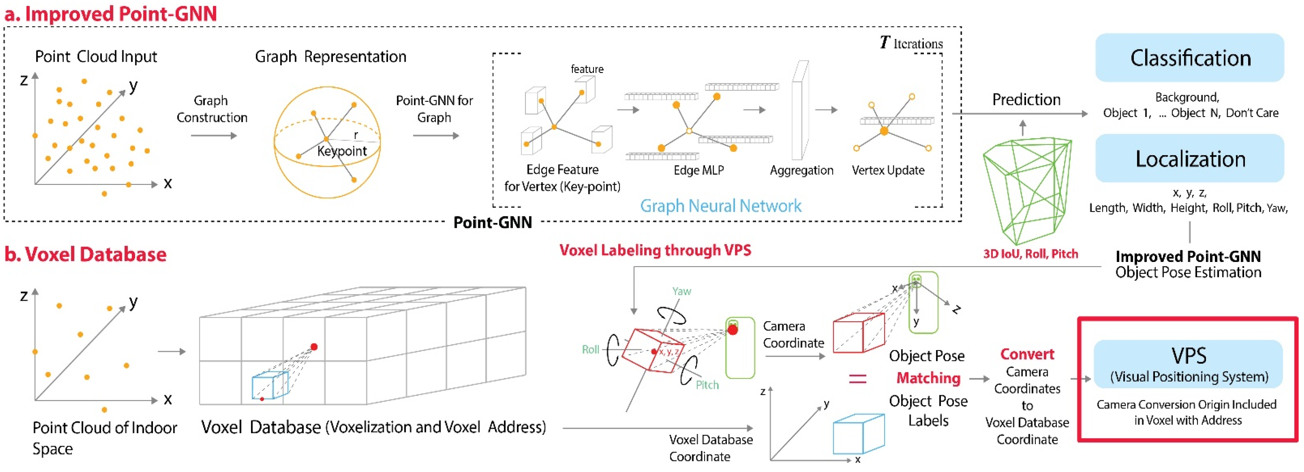
- The proposed method estimates the pose of an object in terms of nine degrees of freedom (DOF) by improving the point-GNN.
- This is a novel method that determines the user’s position as a voxel address in indoor space by matching the object pose label in the defined voxel database with the object pose estimated using the user’s camera position.
2. Related Research
2.1. Point Cloud-Based 3D Object Detection
2.2. D Intersection over Union (IoU)
2.3. VPS
3. Proposed Method
3.1. Point-GNN for 3D Object Pose Estimation
| Algorithm 1 3D IoU values for general 3D-oriented boxes |
| Input: |
| Box n0 is box0 = (x0, y0, z0, l0, h0, w0, ϕ0, θ0, ψ0) |
| Box n1 is box1 = (x1, y1, z1, l1, h1, w1, ϕ1, θ1, ψ1) |
| Applying the Sutherland–Hodgman polygon clipping algorithm: |
| Intersection points between faces of Box n0 and Box n1 |
| Applying the convex hull algorithm: |
| The intersection Volume is computed using the convex hull of all clipped polygons. |
| Union volume is calculated as Box n0 volume + Box n1 volume − Intersection volume |
| Output: Intersection volume/Union volume |
3.2. Voxel Labeling
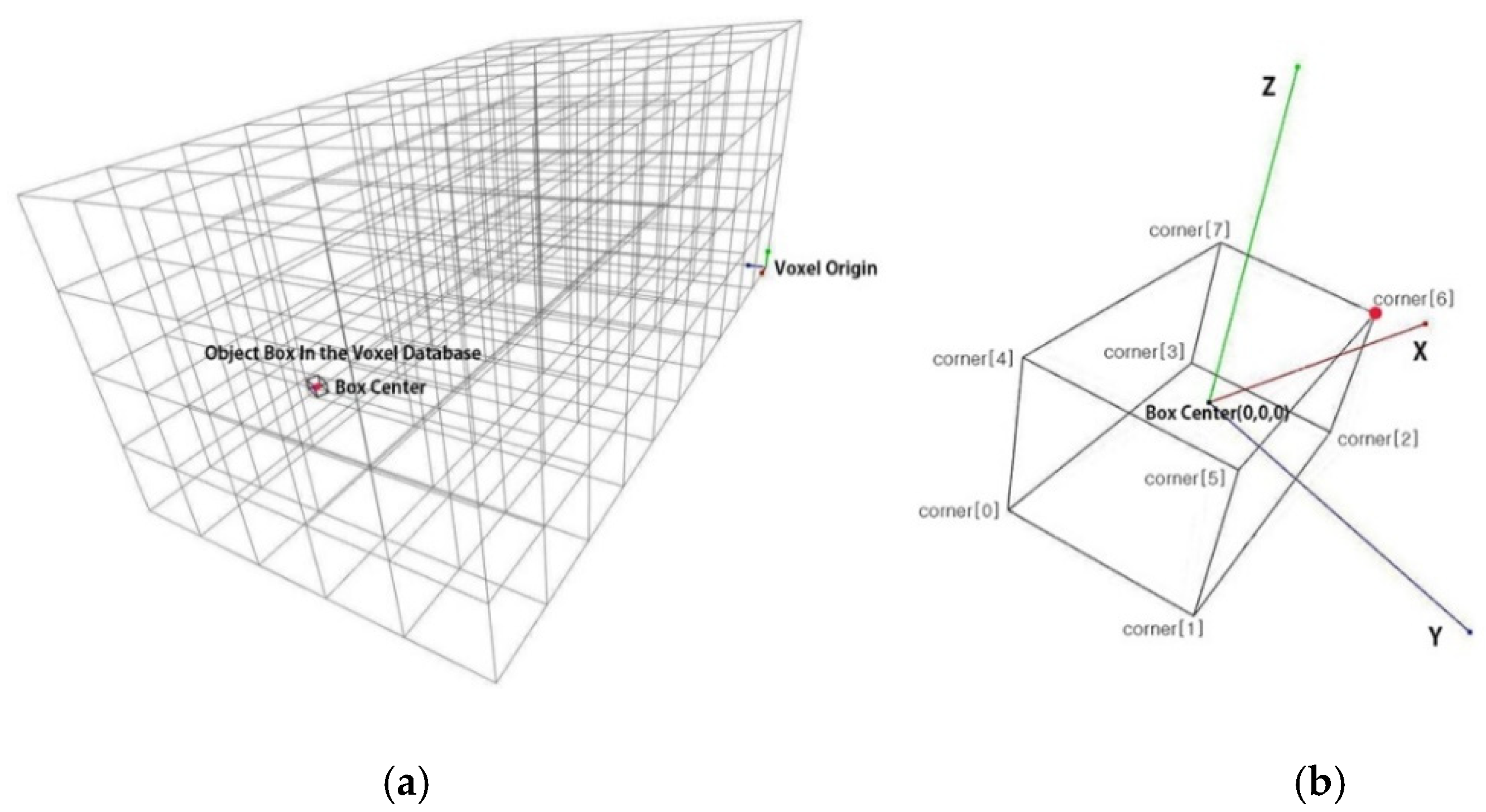
3.2.1. Voxel Labeling in the Point Cloud Database
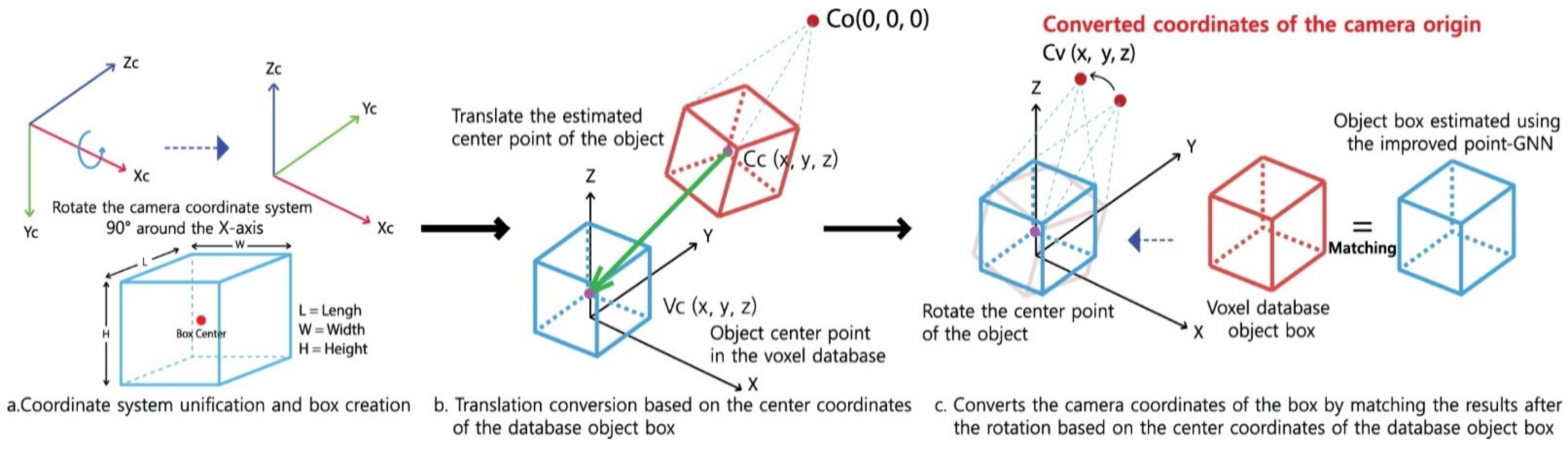
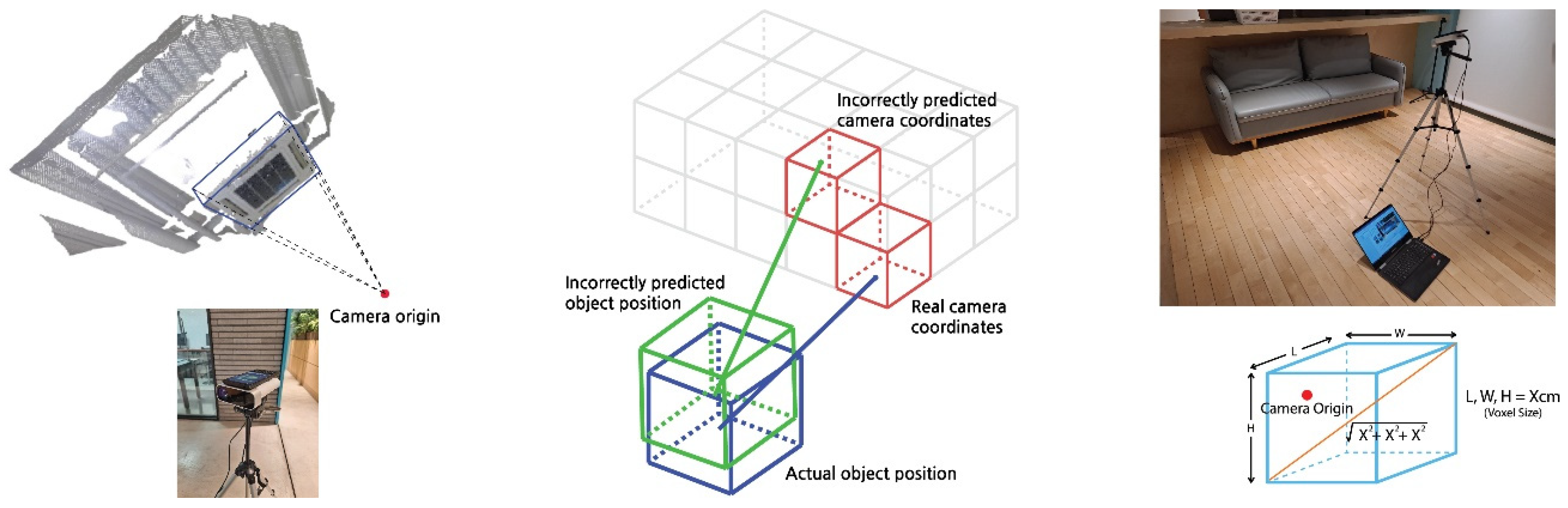
3.2.2. Matching the Object Pose Estimated by Deep Learning with That in the Voxel Database
| Algorithm 2 Calculated rotation matrix between two box 3D vectors |
| Input: |
| box1_vector is box_corners1[6]-box_corners1[0] # box_vector = [ x, y, z ] |
| box2_vector is box_corners2[6]-box_corners2[0] |
| Used dot and cross products to obtain the rotation matrix: |
| C is cross of box1_vector and box2_vector |
| D is dot of box1_vector and box2_vector |
| Norm_box1 is norm of box1_vector # used for scaling |
| if ~ all (C = = 0) # check for collinearity |
| Z is [ [ 0, -C(3), C(2) ], [ C(3), 0, -C(1) ], [ -C(2), C(1), 0 ] ] |
| R is eye(3) + Z + (Z2 X (1-D) / (norm(C) 2))/Norm_box1 2 # rotation matrix |
| else |
| R is sign(D) X (norm(box2) / norm(box1)) # orientation and scaling |
| R is the rotation matrix, so that (except for round-off errors)… |
| R * box1_vector # … equals box2_vector |
| inv(R) * box2_vectory # … equals box1_vector |
4. Experimental Results
4.1. Voxel Labeling
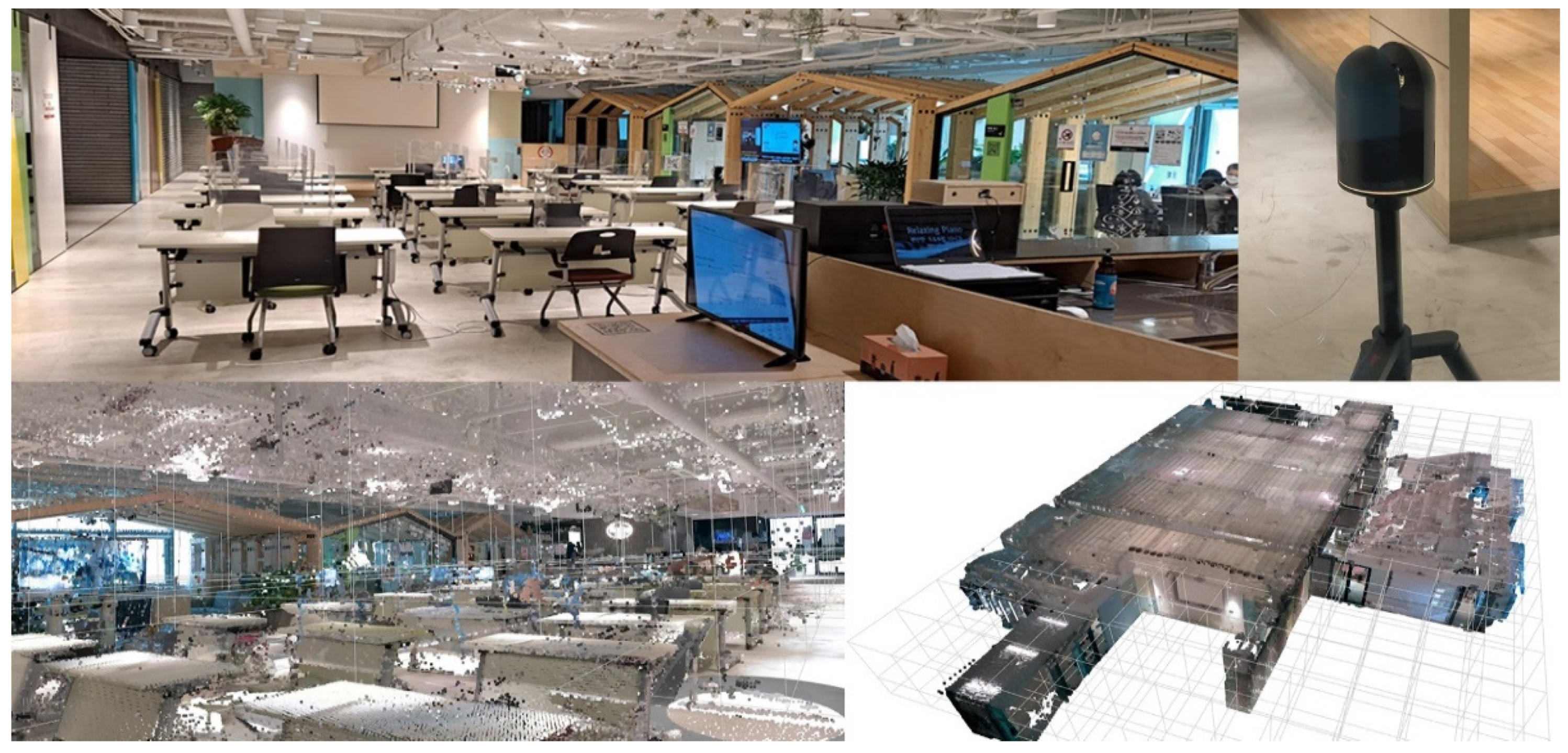
4.1.1. Voxel Labeling in the Point Cloud Database
4.1.2. Results
4.2. VPS Results
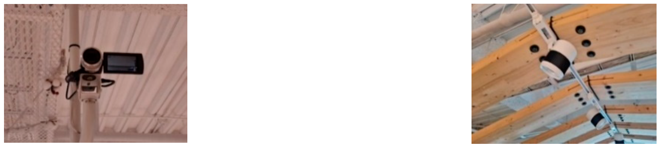
4.2.1. Experimental Setup
4.2.2. Results
4.2.3. VPS Error Rate
5. Discussion
6. Conclusions
Author Contributions
Funding
Institutional Review Board Statement
Informed Consent Statement
Data Availability Statement
Acknowledgments
Conflicts of Interest
References
- Zhang, X.; Wang, L.; Su, Y. Visual place recognition: A survey from deep learning perspective. Pattern Recognit. 2021, 113, 107760. [Google Scholar] [CrossRef]
- Guo, Y.; Wang, H.; Hu, G.; Liu, H.; Liu, L.; Bennamoun, M. Deep learning for 3D point clouds: A survey. IEEE Trans. Pattern Anal. Mach. Intell. 2020, in press. [Google Scholar] [CrossRef] [PubMed]
- Wu, Z.; Pan, S.; Chen, F.; Long, G.; Zhang, C.; Philip, S.Y. A comprehensive survey on graph neural networks. IEEE Trans. Neural Netw. Learn. Syst. 2021, 32, 4–24. [Google Scholar] [CrossRef] [PubMed] [Green Version]
- Shi, W.; Rajkumar, R. Point-GNN: Graph neural network for 3D object detection in a point cloud. In Proceedings of the IEEE/CVF Conference on Computer Vision and Pattern Recognition (CVPR), Seattle, WA, USA, 16–18 June 2020; pp. 1711–1719. [Google Scholar]
- Li, J.; Luo, S.; Zhu, Z.; Dai, H.; Krylov, A.S.; Ding, Y.; Shao, L. 3D IoU-net: IoU guided 3D object detector for point clouds. arXiv 2020, arXiv:2004.04962v1. [Google Scholar]
- Qi, C.R.; Su, H.; Mo, K.; Guibas, L.J. PointNet: Deep learning on point sets for 3d classification and segmentation. In Proceedings of the IEEE Conference on Computer Vision and Pattern Recognition, Honolulu, HI, USA, 21–26 July 2017; pp. 652–660. [Google Scholar]
- Qi, C.R.; Su, H.; Mo, K.; Guibas, L.J. PointNet++: Deep hierarchical feature learning on point sets in a metric space. arXiv 2017, arXiv:1706.02413v1. [Google Scholar]
- Qi, C.R.; Liu, W.; Wu, C.; Su, H.; Guibas, L.J. Frustum PointNets for 3D object detection from RGB-D data. In Proceedings of the IEEE Conference on Computer Vision and Pattern Recognition, Salt Lake City, UT, USA, 18–22 June 2018; pp. 918–927. [Google Scholar]
- Wang, Z.; Jia, K. Frustum Convnet: Sliding frustums to aggregate local point-wise features for amodal 3D object detection. In Proceedings of the 2019 IEEE/RSJ International Conference on Intelligent Robots and Systems (IROS), Macau, China, 4–8 November 2019; pp. 1742–1749. [Google Scholar]
- Shi, S.; Wang, X.; Li, H. PointRCNN: 3D object proposal generation and detection from point cloud. In Proceedings of the IEEE/CVF Conference on Computer Vision and Pattern Recognition (CVPR), Long Beach, CA, USA, 16–20 June 2019; pp. 770–779. [Google Scholar]
- Yang, Z.; Sun, Y.; Liu, S.; Shen, X.; Jia, J. STD: Sparse-to-dense 3D object detector for point cloud. In Proceedings of the IEEE/CVF International Conference on Computer Vision (ICCV), Seoul, Korea, 27 October–2 November 2019; pp. 1951–1960. [Google Scholar]
- Xie, L.; Xiang, C.; Yu, Z.; Xu, G.; Yang, Z.; Cai, D.; He, X. PI-RCNN: An efficient multi-sensor 3D object detector with point-based attentive cont-conv fusion module. In Proceedings of the AAAI Conference on Artificial Intelligence, New York, NY, USA, 7–12 February 2020; Volume 34, pp. 12460–12467. [Google Scholar] [CrossRef]
- Zarzar, J.; Giancola, S.; Ghanem, B. PointRGCN: Graph convolution networks for 3D vehicles detection refinement. arXiv 2019, arXiv:1911.12236. [Google Scholar]
- Chen, Y.; Chen, R.; Liu, M.; Xiao, A.; Wu, D.; Zhao, S. Indoor visual positioning aided by cnn-based image retrieval: Training-free, 3D modeling-free. Sensors 2018, 18, 2692. [Google Scholar] [CrossRef] [PubMed] [Green Version]
- Zhou, Y.; Tuzel, O. VoxelNet: End-to-end learning for point cloud based 3D object detection. arXiv 2018, arXiv:1711.06396v12018. [Google Scholar]
- Liang, M.; Yang, B.; Wang, S.; Urtasun, R. Deep continuous fusion for multi-sensor 3D object detection. In Proceedings of the European Conference on Computer Vision (ECCV), Munich, Germany, 8–14 September 2018; pp. 641–656. [Google Scholar]
- Yan, Y.; Mao, Y.; Li, B. SECOND: Sparsely embedded convolutional detection. Sensors 2018, 18, 3337. [Google Scholar] [CrossRef] [PubMed] [Green Version]
- Lang, A.H.; Vora, S.; Caesar, H.; Zhou, L.; Yang, Y.; Beijbom, O. Pointpillars: Fast encoders for object detection from point clouds. In Proceedings of the IEEE/CVF Conference on Computer Vision and Pattern Recognition (CVPR), Long Beach, CA, USA, 16–20 June 2019; pp. 12697–12705. [Google Scholar]
- Liu, Z.; Zhao, X.; Huang, T.; Hu, R.; Zhou, Y.; Bai, X. TANet: Robust 3D object detection from point clouds with triple attention. In Proceedings of the AAAI Conference on Artificial Intelligence, New York, NY, USA, 7–12 February 2020; Volume 34, pp. 11677–11684. [Google Scholar] [CrossRef]
- Du, L.; Ye, X.; Tan, X.; Feng, J.; Xu, Z.; Ding, E.; Wen, S. Associate-3Ddet: Perceptual-to-conceptual association for 3D point cloud object detection. In Proceedings of the IEEE/CVF Conference on Computer Vision and Pattern Recognition (CVPR), Seattle, WA, USA, 16–18 June 2020; pp. 13329–13338. [Google Scholar]
- Chen, Q.; Sun, L.; Wang, Z.; Jia, K.; Yuille, A. Object as hotspots: An anchor-free 3D object detection approach via firing of hotspots. In Proceedings of the European Conference on Computer Vision, Seoul, Korea, 27 October–2 November 2019; pp. 68–84. [Google Scholar]
- Yang, Z.; Sun, Y.; Liu, S.; Jia, J. 3DSSD: Point-based 3D single stage object detector. In Proceedings of the IEEE/CVF Conference on Computer Vision and Pattern Recognition (CVPR), Seattle, WA, USA, 16–18 June 2020; pp. 11040–11048. [Google Scholar]
- He, C.; Zeng, H.; Huang, J.; Hua, X.S.; Zhang, L. Structure aware single-stage 3D object detection from point cloud. In Proceedings of the IEEE/CVF Conference on Computer Vision and Pattern Recognition (CVPR), Seattle, WA, USA, 16–18 June 2020; pp. 11873–11882. [Google Scholar]
- Zheng, W.; Tang, W.; Chen, S.; Jiang, L.; Fu, C.W. CIA-SSD: Confident IoU-aware single-stage object detector from point cloud. In Proceedings of the 35th AAAI Conference on Artificial Intelligence (AAAI), Online. 2–9 February 2021. [Google Scholar]
- Zheng, W.; Tang, W.; Jiang, L.; Fu, C.W. SE-SSD: Self-ensembling single-stage object detector from point cloud. In Proceedings of the IEEE/CVF Conference on Computer Vision and Pattern Recognition (CVPR), Online. 19–25 June 2021; pp. 14494–14503. [Google Scholar]
- Ren, S.; He, K.; Girshick, R.; Sun, J. Faster r-cnn: Towards real-time object detection with region proposal networks. Adv. Neural Inf. Process. Syst. 2015, 28, 91–99. [Google Scholar] [CrossRef] [PubMed] [Green Version]
- Jiang, B.; Luo, R.; Mao, J.; Xiao, T.; Jiang, Y. Acquisition of localization confidence for accurate object detection. In Proceedings of the European Conference on Computer Vision (ECCV), Munich, Germany, 8–14 September 2018; pp. 784–799. [Google Scholar]
- Liu, L.; Lu, J.; Xu, C.; Tian, Q.; Zhou, J. Deep fitting degree scoring network for monocular 3d object detection. In Proceedings of the IEEE/CVF Conference on Computer Vision and Pattern Recognition (CVPR), Long Beach, CA, USA, 16–20 June 2019; pp. 1057–1066. [Google Scholar]
- Ahmadyan, A.; Zhang, L.; Wei, J.; Ablavatski, A.; Grundmann, M. Objectron: A Large scale dataset of object-centric videos in the wild with pose annotations. In Proceedings of the IEEE/CVF Conference on Computer Vision and Pattern Recognition (CVPR), Online. 19–25 June 2021; pp. 7822–7831. [Google Scholar]
- Sattler, T.; Torii, A.; Sivic, J.; Pollefeys, M.; Taira, H.; Okutomi, M.; Pajdla, T. Are Large-Scale 3D Models Really Necessary for Accurate Visual Localization? In Proceedings of the IEEE Conference on Computer Vision and Pattern Recognition (CVPR), Honolulu, HI, USA, 21–26 July 2017; pp. 1637–1646. [Google Scholar]
- Brachmann, E.; Krull, A.; Michel, F.; Gumhold, S.; Shotton, J.; Rother, C. Learning 6D object pose estimation using 3D object coordinates. In Proceedings of the European Conference on Computer Vision, Zurich, Switzerland, 6–12 September 2014; pp. 536–551. [Google Scholar]
- Brachmann, E.; Krull, A.; Nowozin, S.; Shotton, J.; Michel, F.; Gumhold, S.; Rother, C. DSAC—Differentiable RANSAC for camera localization. In Proceedings of the IEEE Conference on Computer Vision and Pattern Recognition, Honolulu, HI, USA, 21–26 July 2017; pp. 6684–6692. [Google Scholar]
- Valentin, J.; Niebner, M.; Shotton, J.; Fitzgibbon, A.; Izadi, S.; Torr, P.H. Exploiting uncertainty in regression forests for accurate camera relocalization. In Proceedings of the IEEE Conference on Computer Vision and Pattern Recognition, Boston, MA, USA, 7–12 June 2015; pp. 4400–4408. [Google Scholar]
- Shotton, J.; Glocker, B.; Zach, C.; Izadi, S.; Criminisi, A.; Fitzgibbon, A. Scene coordinate regression forests for camera relocalization in RGB-D images. In Proceedings of the IEEE Conference on Computer Vision and Pattern Recognition, Portland, OR, USA, 23–28 June 2013; pp. 2930–2937. [Google Scholar]
- Kendall, A.; Grimes, M.; Cipolla, R. PoseNet: A convolutional network for real-time 6-DOF camera relocalization. In Proceedings of the IEEE International Conference on Computer Vision, Santiago, Chile, 7–13 December 2015; Volume 31, pp. 2938–2946. [Google Scholar]
- Kendall, A.; Cipolla, R. Geometric loss functions for camera pose regression with deep learning. In Proceedings of the IEEE Conference on Computer Vision and Pattern Recognition, Honolulu, HI, USA, 21–26 July 2017; pp. 5974–5983. [Google Scholar]
- Valada, A.; Radwan, N.; Burgard, W. Deep auxiliary learning for visual localization and odometry. In Proceedings of the IEEE International Conference on Robotics and Automation, Brisbane, Australia, 21–25 May 2018; pp. 6939–6946. [Google Scholar]
- Radwan, N.; Valada, A.; Burgard, W. VLocNet++: Deep multitask learning for semantic visual localization and odometry. IEEE Robot. Autom. Lett. 2018, 3, 4407–4414. [Google Scholar] [CrossRef] [Green Version]


| One-Stage Method | Reference | Modality | 3D Object Detection AP | Time (ms) | |||
|---|---|---|---|---|---|---|---|
| Easy | Moderate | Hard | mAP | ||||
| VoxelNet [15] | CVPR 2018 | LiDAR | 77.82 | 64.17 | 57.51 | 66.5 | 220 |
| ContFuse [16] | ECCV 2018 | LiDAR+RGB | 83.68 | 68.78 | 61.67 | 71.38 | 60 |
| SECOND [17] | Sensors 2018 | LiDAR | 83.34 | 72.55 | 65.82 | 73.9 | 50 |
| PointPillars [18] | CVPR 2019 | LiDAR | 82.58 | 74.31 | 68.99 | 75.29 | 23.6 |
| TANet [19] | AAAI 2020 | LiDAR | 84.39 | 75.94 | 68.82 | 76.38 | 34.75 |
| Associate-3Ddet [20] | CVPR 2020 | LiDAR | 85.99 | 77.40 | 70.53 | 77.97 | 60 |
| HotSpotNet [21] | ECCV 2020 | LiDAR | 87.60 | 78.31 | 73.34 | 79.75 | 40 |
| 3DSSD [22] | CVPR 2020 | LiDAR | 88.36 | 79.57 | 74.55 | 80.83 | 38 |
| SA-SSD [23] | CVPR 2020 | LiDAR | 88.75 | 79.79 | 74.16 | 80.90 | 40.1 |
| CIA-SSD [24] | AAAI 2021 | LiDAR | 89.59 | 80.28 | 72.87 | 80.91 | 30.76 |
| SE-SSD [25] | CVPR 2021 | LiDAR | 91.49 | 82.54 | 77.15 | 83.73 | 30.56 |
| Point-GNN [4] | CVPR 2020 | LiDAR | 88.33 | 79.47 | 72.29 | 80.03 | 643 |
| CNN models | VidLoc | HourglasPose | BranchNet | PoseNet2 [36] | Nnnet | VlocNet [37] |
|---|---|---|---|---|---|---|
| Localization error | 0.25 m | 0.23 m | 0.29 m | 0.23 m | 0.21 m | 0.048 m |
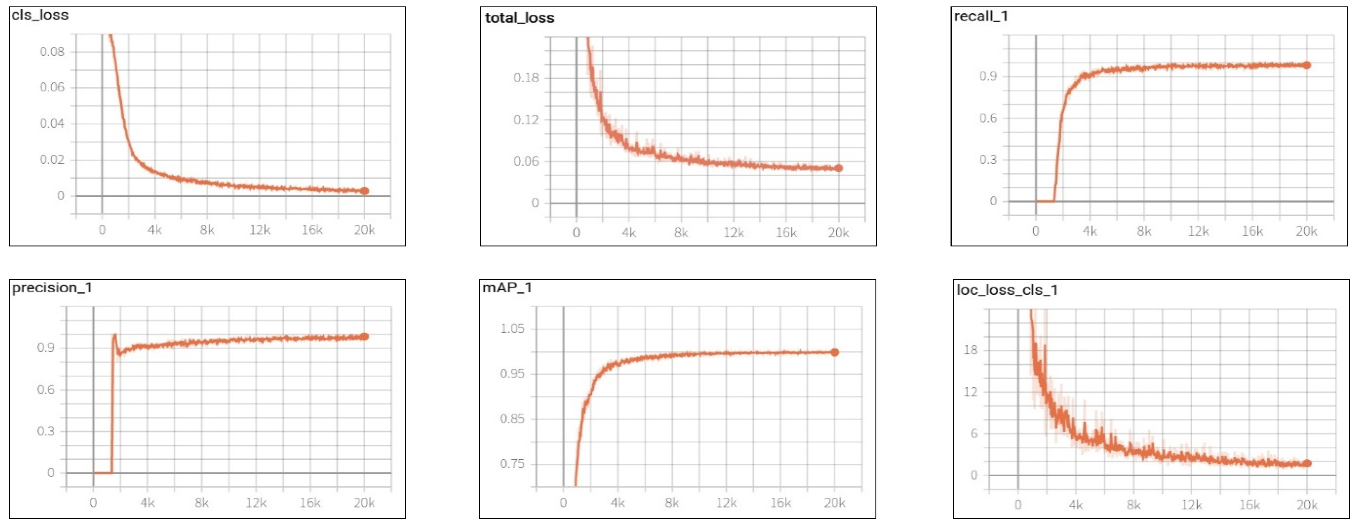
| Loss | Air Conditioner | Chair | Desk | Sofa_01 | Sofa_02 | Flower Table | Flower Pot | Refrigerator | Round Table | Podium Table |
|---|---|---|---|---|---|---|---|---|---|---|
| cls_loss | 0.0060 | 0.0026 | 0.2075 | 0.0101 | 0.0102 | 0.0106 | 0.0077 | 0.0028 | 0.0086 | 0.0030 |
| loc_loss | 0.0135 | 0.0064 | 0.0102 | 0.0164 | 0.0150 | 0.0111 | 0.0244 | 0.0118 | 0.0115 | 0.0117 |
| reg_loss | 0.0393 | 0.0392 | 0.0393 | 0.0394 | 0.0393 | 0.0392 | 0.0394 | 0.0392 | 0.0393 | 0.03926 |
| total_loss | 0.0589 | 0.0482 | 0.0522 | 0.0597 | 0.0613 | 0.0557 | 0.0710 | 0.0539 | 0.0595 | 0.0494 |
| recall | 0.8598 | 0.5937 | 0.9825 | 0.9678 | 0.9861 | 0.9478 | 0.9760 | 0.3636 | 0.8994 | 0.8400 |
| precision | 0.9200 | 0.9047 | 0.9956 | 0.9728 | 0.9666 | 0.9695 | 0.9829 | 0.9939 | 0.8882 | 0.9767 |
| class_mAP | 0.8890 | 0.9092 | 0.9089 | 0.9369 | 0.9382 | 0.8538 | 0.8589 | 0.6939 | 0.9127 | 0.9185 |
| object_loc | 2.6803 | 0.1904 | 2.1270 | 6.2140 | 8.6920 | 1.328 | 2.0200 | 0.2542 | 1.6630 | 0.3188 |
| Log | Details | ||
|---|---|---|---|
| Point cloud (Indoor) | data min _ point | [−9.5453, −1.4278, −12.1236] | Min coordinates in the point cloud |
| data max _ point | [13.6986, 2.6894, 21.7361] | Max coordinates in the point cloud | |
| database min _ point | [−10, −2, −13] | Size of the space expands to the smallest integer | |
| database max _ point | [14, 3, 22] | Maximum size of the space expands to an integer | |
| Voxel | voxel_size | 0.2 m | Voxel size setting (possible up to 0.1 m) |
| max_dim | [120, 25, 175] | voxel_x y z_size | |
| VPS | deep Learning_object _xyz | [−0.0102, −0.0112, −0.4209] | Center coordinates of an object estimated |
| converted_ camera_origin | [−0.0190, −0.0132, −0.4205] | Camera position coordinates in the voxel database | |
| converted_VPS | [8.2809, 1.2867, 2.8794] | VPS coordinates of the voxel database | |
| voxel_points_xyz | [17.8262, 2.7146, 15.0030] | VPS coordinates from the voxel database origin | |
| voxels_numbers | 553,696 | Number of voxels in the voxel database | |
| VPS_voxels_address | 47,450 | User location VPS_voxel address | |
| VPS Error Distance | Air Conditioner | Chair | Desk | Sofa_01 | Sofa_02 | Flower Table | Flower Pot | Refrigerator | Round Table | Podium Table |
|---|---|---|---|---|---|---|---|---|---|---|
| Ours | 0.18 m | 0.18 m | 0.17 m | 0.20 m | 0.30 m | 0.15 m | 0.35 m | 0.14 m | 0.19 m | 0.20 m |
Publisher’s Note: MDPI stays neutral with regard to jurisdictional claims in published maps and institutional affiliations. |
© 2021 by the authors. Licensee MDPI, Basel, Switzerland. This article is an open access article distributed under the terms and conditions of the Creative Commons Attribution (CC BY) license (https://creativecommons.org/licenses/by/4.0/).
Share and Cite
Jung, T.-W.; Jeong, C.-S.; Kwon, S.-C.; Jung, K.-D. Point-Graph Neural Network Based Novel Visual Positioning System for Indoor Navigation. Appl. Sci. 2021, 11, 9187. https://doi.org/10.3390/app11199187
Jung T-W, Jeong C-S, Kwon S-C, Jung K-D. Point-Graph Neural Network Based Novel Visual Positioning System for Indoor Navigation. Applied Sciences. 2021; 11(19):9187. https://doi.org/10.3390/app11199187
Chicago/Turabian StyleJung, Tae-Won, Chi-Seo Jeong, Soon-Chul Kwon, and Kye-Dong Jung. 2021. "Point-Graph Neural Network Based Novel Visual Positioning System for Indoor Navigation" Applied Sciences 11, no. 19: 9187. https://doi.org/10.3390/app11199187
APA StyleJung, T.-W., Jeong, C.-S., Kwon, S.-C., & Jung, K.-D. (2021). Point-Graph Neural Network Based Novel Visual Positioning System for Indoor Navigation. Applied Sciences, 11(19), 9187. https://doi.org/10.3390/app11199187