Data Analytics for Profiling Low-Voltage Customers with Smart Meter Readings

Abstract

The energy transition for decarbonization requires consumers’ and producers’ active participation to give the power system the necessary flexibility to manage intermittency and non-programmability of renewable energy sources. The accurate knowledge of the energy demand of every single customer is crucial for accurately assessing their potential as flexibility providers. This topic gained terrific input from the widespread deployment of smart meters and the continuous development of data analytics and artificial intelligence. The paper proposes a new technique based on advanced data analytics to analyze the data registered by smart meters to associate to each customer a typical load profile (LP). Different LPs are assigned to low voltage (LV) customers belonging to nominal homogeneous category for overcoming the inaccuracy due to non-existent coincident peaks, arising by the common use of a unique LP per category. The proposed methodology, starting from two large databases, constituted by tens of thousands of customers of different categories, clusters their consumption profiles to define new representative LPs, without a priori preferring a specific clustering technique but using that one that provides better results. The paper also proposes a method for associating the proper LP to new or not monitored customers, considering only few features easily available for the distribution systems operator (DSO).

1. Introduction

The electrical load knowledge has always been essential for most applications and studies on the power system regarding network operation and planning. It is well established that it is not sufficient to estimate the total load demand or the total production in a given instant or forecast them in a specific time horizon. The time series of both consumption and generation is imperative for adequately representing the impact of demand coincidence and of the, often low, generation–load homotheticity, which are the causes of voltage regulation issues and power congestions, especially at the medium-voltage (MV) and low voltage (LV) levels where most distributed energy resources (DERs) are connected. This is even more true nowadays since new loads, characterized by coincident peaks of consumption (e.g., home charging of electric vehicles) or by high absorption peaks (e.g., heat pumps or cooking appliances) are increasingly frequent. Moreover, the massive diffusion of non-programmable renewable energy sources (RES), dispersedly connected to the distribution system, causes severe operation problems, and gives a leading role to the flexibility of demand, which is crucial for the success of the energy transition. Both conventional and emerging stakeholders of the power system, transmission and distribution systems operators (TSOs and DSOs), regulators, market players such as balance responsible parties, and aggregators are interested to accurately model the behavior of customers with load profiles (LPs).

LPs are patterns of electricity load consumption of a customer or a group of customers over a given period that have been extensively used for many years. Generally, LPs are obtained from historical data or measurement campaigns, suitably elaborated for defining representative or typical consumption shapes. Unfortunately, the LP updating is not sufficiently frequent, and, often, LPs refer to customers that no longer exist. Moreover, the current LPs are often based on measurement campaigns that involve a small number of customers not significant as a statistical sample of a defined ambit (e.g., a region or a country). Such LPs can capture only a portion of the end-users and cannot represent modern consumers, particularly the new prosumers. Indeed, even the most accurate LPs that associate with homogeneous groups of end-users one profile per season and the day (workday, weekend, pre-holiday, holiday), generally obtained by averaging the relevant samples, are not so realistic. These models consider daily curves applicable to groups of consumers subdivided on the basis of the contract or economic activity (i.e., residential, agricultural, industrial, or tertiary) [1]. Nevertheless, assuming a certain homogeneity among end-users and neglecting the actual variability among consumers’ consumption habits belonging to the same category is acceptable for almost all economic activities but is not valid for residential consumers. The residential users exhibit a tremendous variance of load profiles that depends on several exogenous factors (i.e., household size, the number of persons living in a household, net income and employment status, level of education, etc.) [2,3,4]. Hiding single customers behind a large and non-homogeneous group’s average behavior leads to significant errors in distribution studies. One typical example is represented by the time coincidence of the demand in residential neighbors that is considerably smaller than the one that can be achieved by superimposing the same load profile several times. Consequently, models that associate to all the customers belonging to the same category one day profile only, even differentiated by season or typical day, result as inaccurate, mainly if the category is residential.

Nowadays, new and more accurate measurements can be gathered from the advanced metering infrastructure (AMI) that uses the second generation of smart meters. In the current network operation practice, the data provided by the intelligent metering are not fully involved, and the resort to such accurate and updated measured data may be addressed for producing new load profiles of both active and reactive power, more realistically than in the past [2,3,5]. These models should be capable of capturing the different behavior of customers by using further information. Such information may not be necessarily too detailed and should not adversely affect the customers’ privacy rights by exploiting ad hoc techniques to deal with a vast amount of data [2,5,6]. As an example, new LPs could be obtained by filtering field data with geographic information to find correlations with the climate conditions (the use of electricity is different in the northern, colder, areas than in the southern ones), with socio-demographic characteristics (e.g., income, education level, social status), etc.

In this paper, an approach for obtaining typical LPs from a database of measured data is proposed. The method is based on well-known clustering techniques used for grouping in clusters similar behaviors of end-users belonging to the same category. The goal is to obtain a set of load consumption shapes that could capture the diversity within the same customer category, potentially homogeneous. The methodology consists of a two-stage procedure that aims at characterizing the single customer, and then it groups different customers into classes. Both stages may be performed with clustering techniques, as detailed in the next sections. The results, i.e., the sets of LPs associated with each customer’s category and differentiated between the typical days in the year (i.e., three typical days for each season), can be used for representing existing customers of a given network but also aspire to foresee the behavior of new customers that can be supplied by a new portion of the distribution system. The bullet points below highlight the main advancements compared to the state of the art that can be regarded as the main procedure’s point of strength:

(i)

capability to deal with large databases from the field (much larger than the ones dealt by almost the totality of methods proposed by the literature);

(ii)

output-based approach, i.e., it does not a priori prefer a specific clustering technique but uses the one which provides the better results;

(iii)

accurate association of an LP to a new or a non–monitored existing customer or to a group of customers of the same network considering only few features known by the DSO.

From an application point of view, it is worth mentioning that the application of the procedure has produced new and updated LPs, on the basis of recent and large databases gathered from extensive measurement campaigns. The new LPs capture much of the Italian load diversity and can be used to model the load consumption of a modern and developed country provided that a suitable scale factor is used. The more accurate modelling of load diversity reflects on a more accurate representation of load coincidence with an immediate impact on planning studies for expansion studies.

The rest of the paper is organized as follows. Section 2 briefly reviews the current state of the research field on the methods for assessing load profiles; in Section 3, the proposed approach is described in detail; Section 4 reports the results of the application of the proposed approach to databases gathered from real measurement campaigns; in Section 5, one example of application of the LPs is proposed for demonstrating the validity of the approach. Finally, the conclusions are reported.

2. Load Profiling

In the literature, several techniques have been proposed for obtaining LPs. Each method is specialized for the specific study’s goal or on the group of customers represented [3,6,7].

Models for network planning generally use a probabilistic approach by exploiting probabilistic load flow (PLF) calculation algorithms, Monte Carlo methods, or analytical methods [4,8]. The PLF input variables (load and generation) are commonly represented by suitable probability density functions (PDFs). However, it is not straightforward to represent each load and generator with a PDF. The dynamic nature of consumer behavior is heavily time-dependent. Correlations and time dependencies should be considered simultaneously to ensure a good characterization of load and generation [8]. For instance, other studies, with the aim of elaborating market balancing mechanisms in competitive frameworks or for devising marketing strategies, exploit predictive analyses, such as the multi-linear regression analysis. With such analysis, they avoid the considerable investment of putting half-hourly metering into every market customer and calculate the profile coefficients of several customer classes [9]. In this case, customer behavior profiling can be used as a useful tool for tariff rate formulation. Bottom-up methods can be performed for (smart) home energy systems design. They aim to build load profiles or PDFs of specific electrical devices by using detailed information on devices’ usage and elaborate and combine them to make profiles that aspire to represent other households and areas [1,3,8]. Any probabilistic or predictive method produces results affected by a certain, sometimes measurable, uncertainty level by seeking a compromise between computational burden and accuracy. On the other hand, the data gathered from smart meters may help and reduce such uncertainty.

Among all the techniques and regardless of the database origin (any meters, new or old), clustering techniques have been extensively applied to measured consumption patterns of end-users to categorize customers and define typical LPs for each category. Clustering allows grouping similar load patterns in classes. Then, once the profiles are grouped, each class’s centroid can be chosen as the LP of the cluster whose it belongs. Moreover, a neighborhood of the centroid identifies the subspace where similar load profiles can be found.

Various clustering algorithms have been proposed in the literature, i.e., deterministic, statistical, and artificial intelligence methods. Clustering methods can be split into hierarchical and partitional methods [10]. The hierarchical methods provide a dendrogram of nested clusters that allows for an overview of all possible clustering outcomes. Such techniques can be based on agglomerative or divisive approaches. In the agglomerative approach, the clustering process starts by defining a cluster for each individual, and these clusters are then iteratively merged according to the respective similarity. Conversely, in the divisive approach, a unique cluster formed by all the dataset individuals is iteratively split. The partitional clustering methods do not provide clusters as an outcome but a unique partition of the dataset. The key idea of these methods is based on optimizing a criterion function by alternating the initial partitioning of individuals. k-means is the simplest and most popular partitional clustering algorithm [10,11,12,13].

Past and recent literature show a great diversity in terms of approaches, used databases, clustering algorithms (e.g., partitional, hierarchical, fuzzy, neural networks), and similarity/dissimilarity criteria (e.g., Euclidean distance, mean of the inner distance, mean square error, mean index adequacy, clustering dispersion indicator, the within-cluster sum of squares to between-cluster variation) [14]. The most appropriate clustering technique should be chosen according to the analysis’s goal and the dataset’s characteristics [10]. The authors of [14] proposed a general framework for supporting the analyst in selecting the most common algorithms used for load profiling through a multi-attribute decision-making technique for considering several conflicting criteria. The analysis’s outcome highlights that the partitional algorithms (such as k-means) have better performance in classification validity. In contrast, hierarchical methods show a lower computational time and complexity.

To provide a brief overview about the state of art of load profiling research activities and for highlighting the novelties and the strengths of the proposed approach, several recent papers regarding this topic were surveyed. Modified versions of the k-means algorithm dedicated to the load profiling analysis are proposed in [15]. The article describes a multi-stage load profiling framework in which the k-means algorithm plays a crucial role. The two versions of the modified k-means algorithm had an updated initialization stage, the initial centroids were selected linearly and not randomly, and extended quantiles were considered. The effectiveness of the proposed algorithm was verified on a limited set (i.e., 150) of customers of various types. A scalable load profiling algorithm was proposed in [16] to undertake big data processing. A growing self-organizing map was implemented on a parallel and scalable computing platform to achieve high data processing volumes in real time. The dataset analyzed consisted of about 10,000 Australian residential customers’ readings measured with 30 min of sampling time. A method for the stochastic modeling of the smart meter data is proposed in [17]. The difficulties related to managing the high volume of data provided by the large-scale deployment of smart meter data were relieved by linearizing the energy consumption patterns. The linearized consumption patterns were then analyzed using a proposed clustering algorithm based on k-means, enhanced for improving the analysis of profiles characterized by a high intra-cluster similarity. In [18], a load profiling-based methodology to support the DSO investment decisions is proposed. The method uses hierarchical clustering for identifying similar load profiles at the distribution substation level for representing all days of a given period. The entire year was characterized by 12 typical load profiles obtained as the resulting clusters’ centroids. A Markov process was used for representing the stochastic grid behavior starting from the typical profiles’ behavior. The use of density-based spatial clustering of applications with noise (DBSCAN) as clustering algorithms is proposed in [19], together with the hierarchical approach, in order to capture customers’ electric behavior and build typical load profiles, as well as in [20], for identifying suitable electricity retail price for residential customers. In [19], DBSCAN was used for creating a representative profile for each primary substation (i.e., high voltage HV/medium voltage MV interface), starting from the data obtained from daily measurement. The hierarchical approach was exploited for identifying the similarities among the different representative shapes of the primary substations. The optimal number of typical load profiles suggested for describing the Portuguese territory’s primary substations was found by combining the clustering analysis outcome with geographic information and business intelligence. In addition, a statistical analysis of end-users’ historical consumption regarding around 3000 profiles was conducted to better capture their consumption regularity and associate a single profile [20]. In [21], a hierarchical clustering approach was used for defining representative daily profiles from the measurement collected from tens of thousands of secondary substations distributed over the Portuguese territory. The representative daily profiles were then used for building a probabilistic distribution function that modeled the power consumption of each secondary substation in each instant of the day. The described methodology aimed to characterize the consumption patterns of existing and new secondary substations (i.e., LV/MV interfaces) in a probabilistic way. The article [22] focuses on reducing computational complexity of load profiling by preserving the information content in load patterns. To this aim, a method to analyze fine-grained smart meter data on the basis of singular value decomposition and wavelet energy entropy is proposed. Five features are identified as the compromise representation of load profiles for reducing computational cost while preserving accuracy. In this paper, the authors made use of principal component analysis (PCA) for reducing the dimensionality of the data to be clustered. In [23], load profiling was undertaken for gathering information useful for designing demand-side flexibility strategies. The k-means algorithm was used to segment households according to the electricity pattern while the household characteristics were studied to determine the influences on the electricity consumptions. In [24], load profile segmentation was developed for market settlement purposes. The hierarchical clustering approaches with Euclidean and dynamic time waring distances and average and Ward’s linkage criteria were compared offline for analyzing measured consumption profiles of residential, commercial, and industrial consumers. Furthermore, the partition obtained by imposing several final numbers of clusters (5, 10, 15, and 20) were studied offline for identifying the most convenient set up. The authors of [25], starting from one year of smart meter electricity demand data from 656 households in Switzerland, compared two clustering approaches (k-means using daily load shape and k-means using daily profile features). The use of the daily profile features allowed to identify three distinct patterns over the course of the day, which challenges the assumption made by Swiss energy regulation that one standard pattern fits all homes [25]. In [26], three algorithms are compared: k-means, bisecting k-means clustering, and Gaussian mixture model-based clustering using a dataset of about 4000 buildings from different climatic zones and characterized by different purposes. Three fundamental load shapes were identified and to each building a dominant profile is assigned. In [27], daily profiles for typical buildings were identified using a two-level clustering on the basis of Gaussian mixture model and on hierarchical clustering. Two-year hourly electricity consumption of 40 university buildings with different purposes were processed.

The comparison between the proposed approach and the surveyed literature may be made considering different aspects, e.g., (i) the size of the used database (i.e., duration of the measurement campaign, number and variety of customer category investigated), (ii) the association of one or more than one profile to customers belonging to the same category, (iii) the choice of the optimal clustering algorithm among different techniques (during the load profiling process or offline), and (iv) the ability of assigning a proper LP to a single or (v) to a group of customers.

The dataset size used by the surveyed papers spans from the yearly profile of one industrial consumer only [14] to a few tens of two customer categories (residential and small enterprises users) [22], to hundreds of consumers without category characterization [15] or residential only [24,25], to a few thousand (i.e., 2771 in [20], 5000 in [17]), to a few tens of thousands of residential customers only [16,23]. Other studies refer to load profiles of aggregated customers, i.e., at level of primary substations (few hundreds in [19]), or at level of secondary substations (tens of thousands in [21]), or referred to buildings (tens in [27], thousands in [26]). An outstanding database is used in [18]—it includes over 6 million LV clients. The research activity described in this paper is based on two large and recent datasets of measured daily profiles that refer each to a one-year measurement campaign and initially included both over 100,000 monitored end-users. By limiting the study to the customers with both profile and type of contract known, the databases are reduced to 56,034 and 31,790 LV customers, respectively. Therefore, considering the reviewed articles, the databases used in this paper, even reduced, are at the top levels in the ranking and only the activity described in [18] concerns a larger dataset.

Moreover, considering the load profiling approaches in the reviewed literature, even if more than one clustering technique is exploited in some papers, the use of one clustering technique only for the load profiling process is common [14,15,16,17,18,20,21,22,23,24,25]. In [19] and [27], two different clustering techniques were used in a sequential way, while in [26], three different algorithms were compared offline. One of the contributions of this paper is the improvement of the clustering process, which relies on the online comparison of two different clustering techniques (k-means vs. hierarchical), which are based on different approaches (divisive vs. agglomerative). These two techniques are applied in parallel considering different partition set-up. The overall outcome of the clustering approach depends on the best performances achieved by the two algorithms. The optimal clustering set-up is identified according to the best values of the validity index achieved.

Two reviewed papers aimed at enhancing the performances [15] or providing a comparative analysis [14] of acknowledged algorithms. The papers [16,17,22,23] addressed the topic of identifying common patterns among one category of customers only, while more than one category was studied in [20,24,25,26,27]. In this paper the electric behavior of all the categories of Italian LV customers is studied (i.e., industrial, commercial, agricultural, and residential). As in [18,19,21] for the Portuguese power system, the aim of the activities described in this paper is to characterize the typical electricity behavior of the Italian customers by assigning to each category more than one typical profile, thereby improving the state of art of customer segmentation practices. Future works would be devoted to compare the typical load profile of customers of different European Countries.

Once a typical pattern is identified for the analyzed profiles in the dataset, the load profiling activity poses the problem of assigning these typical load profiles to customers that do not belong to the analyzed dataset. This stage is not addressed in [14,15,16,17,19,21,22,24,27]. In [18], Markov chains were proposed for creating synthetic models of the MV/LV and HV/MV interfaces to be used for analyzing the network at the higher voltage level. In [25], the obtained daily curves were used for highlighting the variability of the household’s electricity use. The association of the typical load pattern to new customers was based on external information (e.g., income, education, dwelling size) in [23], and historical data in [20], while in [26], the buildings were assigned to the dominant clusters (i.e., those that occur more frequently, identified by using the entropy computation). In this paper, the association of the most suitable typical load profile to new customers (i.e., those which are not part of the analyzed dataset) is made, considering only features easily available for the DSO (e.g., annual energy, rated power, monthly peak). Thus, it represents a concrete improvement of the state of the art and a step forward in the field of load profiling, since the outcome of the research activity can be exploited in real-life applications, considering the current transitional period and the near with the possible functionalities of advanced metering infrastructures only partially enabled.

Clustering for Assessing Load Profiles

Although each clustering algorithm has its peculiarity, a general approach for the clustering analysis of load profiles can be defined. As proposed in [28], load consumption patterns can be classified by applying four main steps:

• Consumption pattern acquisition. The consumption pattern of each end-user has to be firstly gathered using the metering infrastructure. Two issues arise from this step that can alter the entire process of classification—the duration of the measurement campaign (it should last at least one year to capture the seasonality of the variations in the end-users’ consumption) and the representativeness of the sample (that should be constituted by many customers spread in the area that the study aims to represent to avoid the risk of having no statistical value). At the end of the measurement campaign, the initial database is constituted. Still, many spurious measures or loss of communications may occur during the measurement campaign. Thus, the initially formed database must be processed to detect and eliminate bad data and create a more reliable and robust database.
• Representative features selection. In this phase, the selection of the representative features of the dataset individuals is performed. Features can be time-domain data, load shape factors, frequency-domain coefficients, projection analysis method coefficients, etc. [10,29]. In the paper, this step has been applied to characterize the behavior of a single customer (i.e., a given customer can exhibit load profiles very different one day from each other day, even during the same type of day) and to discover the similarity of the consumption shapes of different end-users. The number of identified features can grow in number, and thus techniques such as principal component analysis (PCA) may be conveniently used for reducing the number of features [30].
• Clustering application. Suitable clustering algorithms must be applied to the dataset of features selected in the previous step. With this step, in the proposed approach, it is possible to identify the single customer’s most frequent behavior by grouping similar load shapes within the dataset of the given end-user or to group the customers of the database into classes. Thus, each cluster’s identified centroid may alternatively be used for selecting the LP that characterizes the single customer or may become the LP associated with the customers belonging to the cluster.
• Validation. The last step is devoted to validating the clustering process by demonstrating its effectiveness with ad hoc tests.

Data pre-processing can be performed before the application of a clustering algorithm to improve the success of clustering. Pre-processing means, for instance, choosing a specific load condition (i.e., selecting a specific seasonal period or a type of day) and defining an initial partition in macro-classes according to external features (nominal power, climatic zone, contract, etc.) [28,29].

3. Proposed Approach

The paper presents a novel methodology that applies the four steps for classification described in Section Clustering for Assessing Load Profiles. The accuracy of load profiling obtained using the proposed method is higher than with other approaches proposed in the literature.

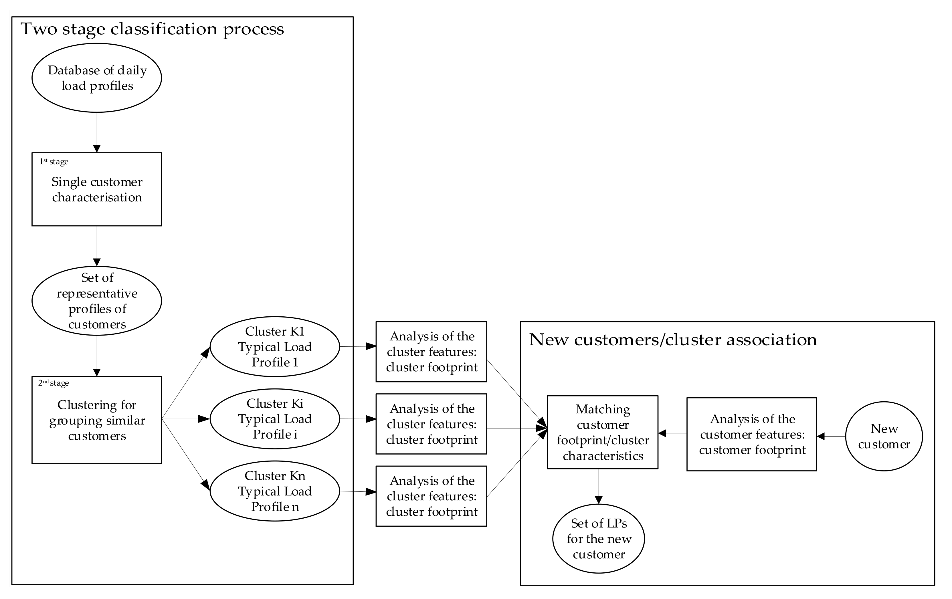
Figure 1 shows a simplified flow chart of the proposed methodology. Once the dataset has been acquired (i.e., first step), the critical features selected (i.e., second step), and the data elaborated for facilitating the purposes of the next steps, the proposed two-stage classification process can be performed. The process starts from the database of available profiles and ends by generating sets of typical LPs (each set is relevant for a given group of customers and for a specific typical day, i.e., commercial customer’s winter workdays).

At first, the process characterizes each customer by defining its representative LPs (i.e., the first stage of the classification process, as described in Section 3.3.1). Then, the similarity among representative LPs of different customers is analyzed. A partition of clusters that groups similar representative LPs is obtained (i.e., the second stage of the classification process, see Section 3.3.2). For each cluster, a typical LP is calculated; each typical LP represents the consumption pattern of all customers included in the related cluster.

A second path, subordinated to the end of the classification process, aims to assign to new customers one of the typical LPs generated through the main path. Through this path, starting from his/her specific features that define his/her footprint, any new customer whose load profile is unknown could be associated with one particular cluster (i.e., by following the lateral path in Figure 1 and described in Section 3.4). The association can be made by matching the cluster footprint, obtained by analyzing the features of the resulting clusters, and the customer’s footprint.

The proposed approach is detailed in the following subsections.

3.1. Data Acquisition

As mentioned above, the clustering algorithms are data-driven techniques, and thus the more accurate, complete, and recent the available database, the better the quality of the results. Data to be acquired are the measured patterns of the active power delivered to the customers. Often, only limited information related to the customer electrical supply contract is provided (rated power, tariffs, type of contract, etc.).

Generally, due to privacy and security reasons, it is uncommon to have available databases with useful extra exogenous information, especially for the DSOs that are regulated bodies and do not run any commercial activity. Still, in many cases, the available databases could even be lacking in the active power samples.

3.2. Feature Selection and Data Pre-Processing

The selection of the features that can impact end-user’s electrical behavior is a sensitive matter. Often, the choice necessarily falls onto the limited information provided by the available database. Such initial selection can also impact the phase of association of new customers to a set of LPs. In the literature, various studies on the factors that influence the final electricity consumption, which should be considered key features for modeling the load demand by building representative LPs, have been proposed. Factors that strongly impact the final use of the electricity are type of contract (e.g., in many cases, distinguished only into residential and other usages) or the rated power. Still, many other exogenous features could also be important for differentiating the LPs. For residential customers (the most difficult to deal with), the most relevant socio-demographic factors are the household size [4,31], the type and number of electric appliances in each home and their usage [31], the number of persons living in the household, how many of them are expected to be at home at the same time [32], salary [31], and employment status [4]. Finally, the weather is recognized as having a significant influence on electric consumption, and its role would be included in any analysis of customer electrical load patterns [32,33].

Unfortunately, most of the databases do not include exogenous information about the customers or their habits, home appliances, etc. Thus, the proposed approach’s idea is to operate a first segmentation that filters the features that can mainly be considered responsible for the load shapes’ diversity. The first segmentation aims at considering, one by one, groups of customers nominally homogeneous (e.g., the same type of supply contract or same geographic area). In particular, the main dichotomy is made between residential and other usage contracts. Moreover, among the residential customers, the difference between main and secondary residence contracts and, among the other usage contracts, depending on the economic sector (i.e., agricultural, industrial, or commercial customers), are considered. Finally, in this paper, as is the common practice of DSOs and without affecting the generality of the approach, the year into quarters is split, and three typical days for each quarter are considered (i.e., working days, Saturdays, Sundays, and holiday), as in [1,34]. It is worth noticing that each formed group of customers and, within the same group, each typical day is independently handled.

Nevertheless, the features to be clustered within the same group of customers remains to be selected. Since the proposed approach aims to discriminate between the shapes of the customers’ daily consumption profiles belonging to the same category, the selected features can be the time-series of the load consumption pattern. In this work, the only active power measured profiles are considered, but the same procedure can be applied to the reactive power patterns.

Since the load consumption database contains raw data, a pre-processing phase is indispensable for removing missed samples and bad data, as well as reducing the number of features to be handled in the next steps. For instance, for filling the missing data in a given customer’s time series, the samples’ average relevant to the same time interval in the same typical day is used. This pre-processing activity is crucial but long and burdensome, and the reliability of the obtained outcome strongly influences the accuracy of the following stages. The result of this step is new subsets of load-measured profiles related to customers for which there are in the database enough data for considering them “valid” to be analyzed.

3.3. Two-Stage Classification Process

3.3.1. Customer Profiling (Stage 1)

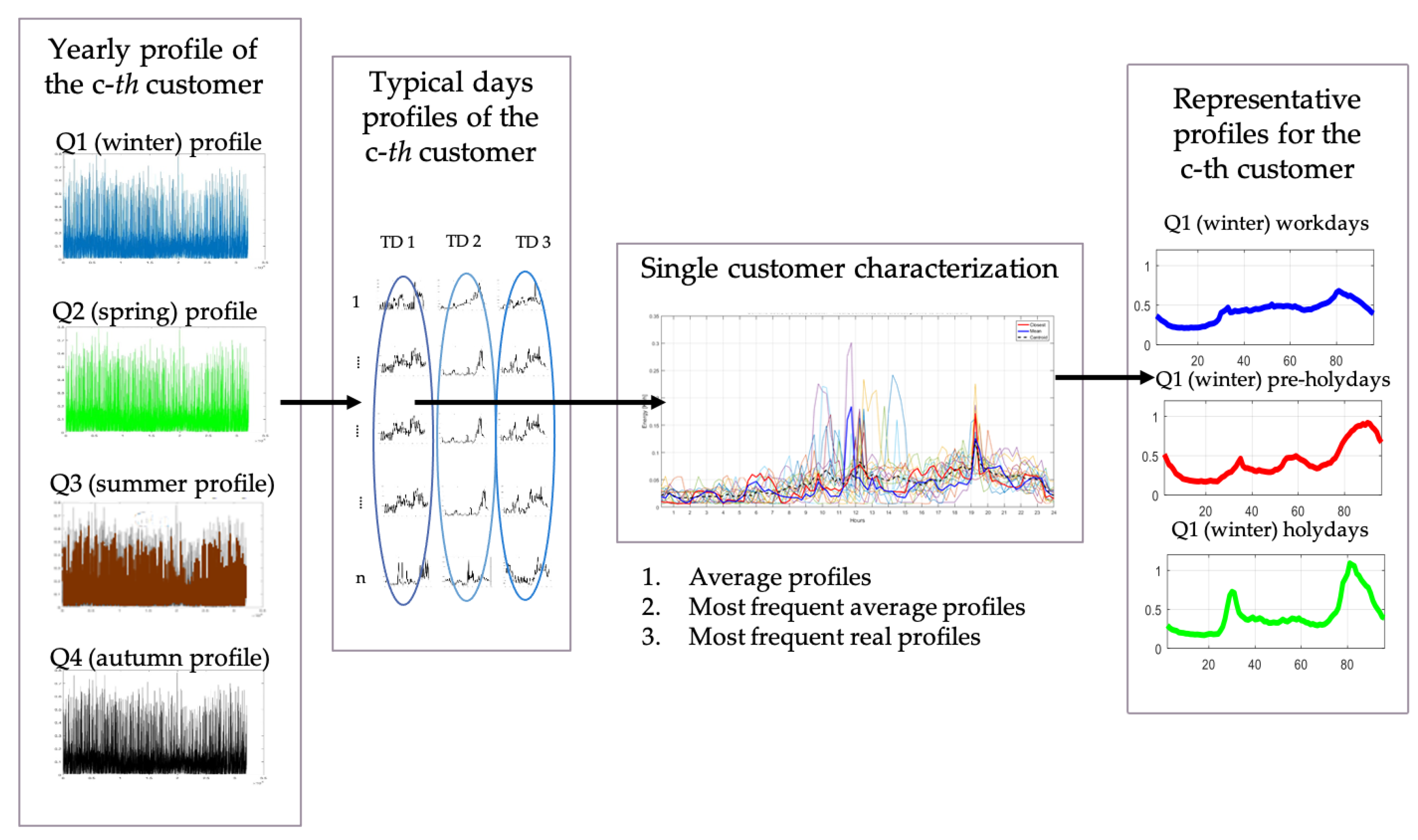
The objective of stage 1 is associating each consumer with features that are typical of the shape of the consumption profile (Figure 2), e.g., the time of morning and evening peaks, the deepness of the valleys in the curve, and the maximum difference between peak and off-peak consumption. Classical features such as customer’s annual and daily consumption commonly are less important than the shape of the consumption.

As mentioned above, the consumption patterns are split into four quarters; in each quarter, data analysis identifies the consumption curves for workdays, Saturdays, and holidays. Year quarters reflect with a good approximation the seasonality (Q1—winter, Q2—spring, Q3—summer, Q4—autumn) [1].

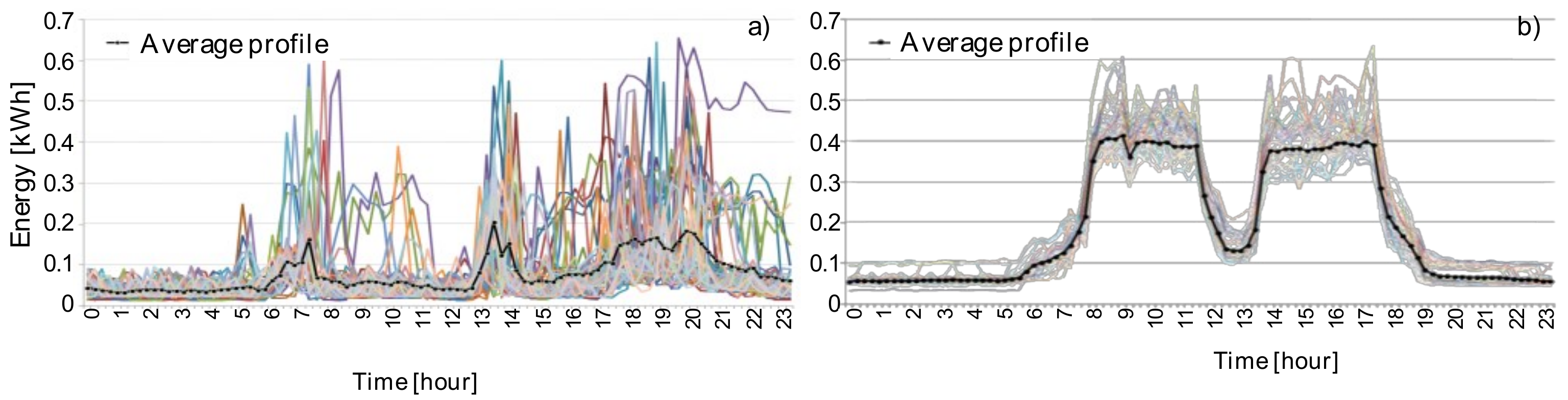
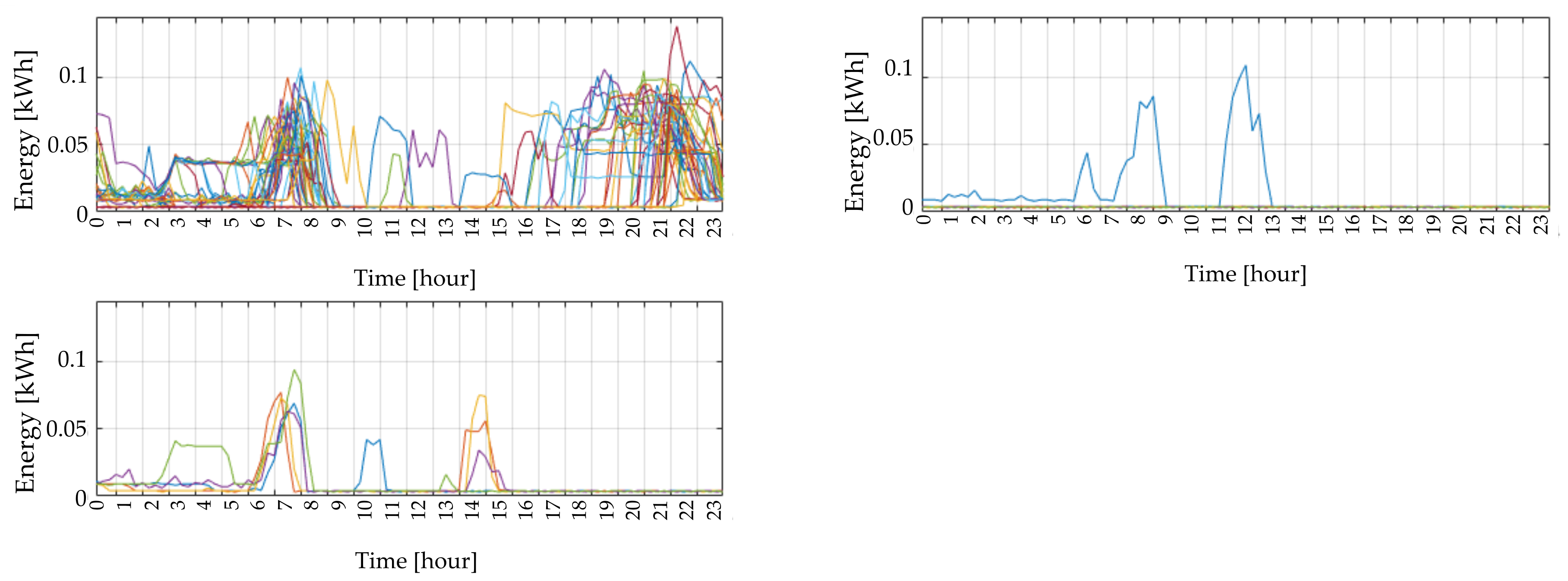
Customer’s consumption is different in all days of the same category. Differences are particularly significant for the residential customers that may exhibit very different load curves one day from another, even of the same type. In Figure 3a, given residential end-users’ consumption patterns in the winter weekdays are reported (the black curve is the average profile). For industrial, commercial, and tertiary customers, these differences are less significant since the consumption is prevalently linked to job activities (Figure 3b).

The methodology needs to associate a single profile to each customer for any quarter of the year and for any category of the day. Several methods have been tested to minimize the risk of losing significant information. In this paper, the most frequent average profiles assignment was implemented—for each customer, the consumption patterns during a specific typical day are clustered with Ward’s linkage hierarchical clustering algorithm [12,35]. The optimal number of clusters is identified according to the Davies–Bouldin index (DBI) minimum value, calculated for a limited number of the dendrogram’s resulting levels [12,35]. These clustering process results are classes of daily profiles with different shapes for the same typical day and for the same customer. The profile associated with customer behavior is the centroid of the most populous class, which is the average of the most frequent profiles.

The representative consumption pattern is constituted by several samples dependent on the intervals on which is discretized the day (i.e., 96 samples for a sampling rate of 15 min) for each of the 12 typical ones associated with each customer

3.3.2. Clustering for Grouping Customers (Stage 2)

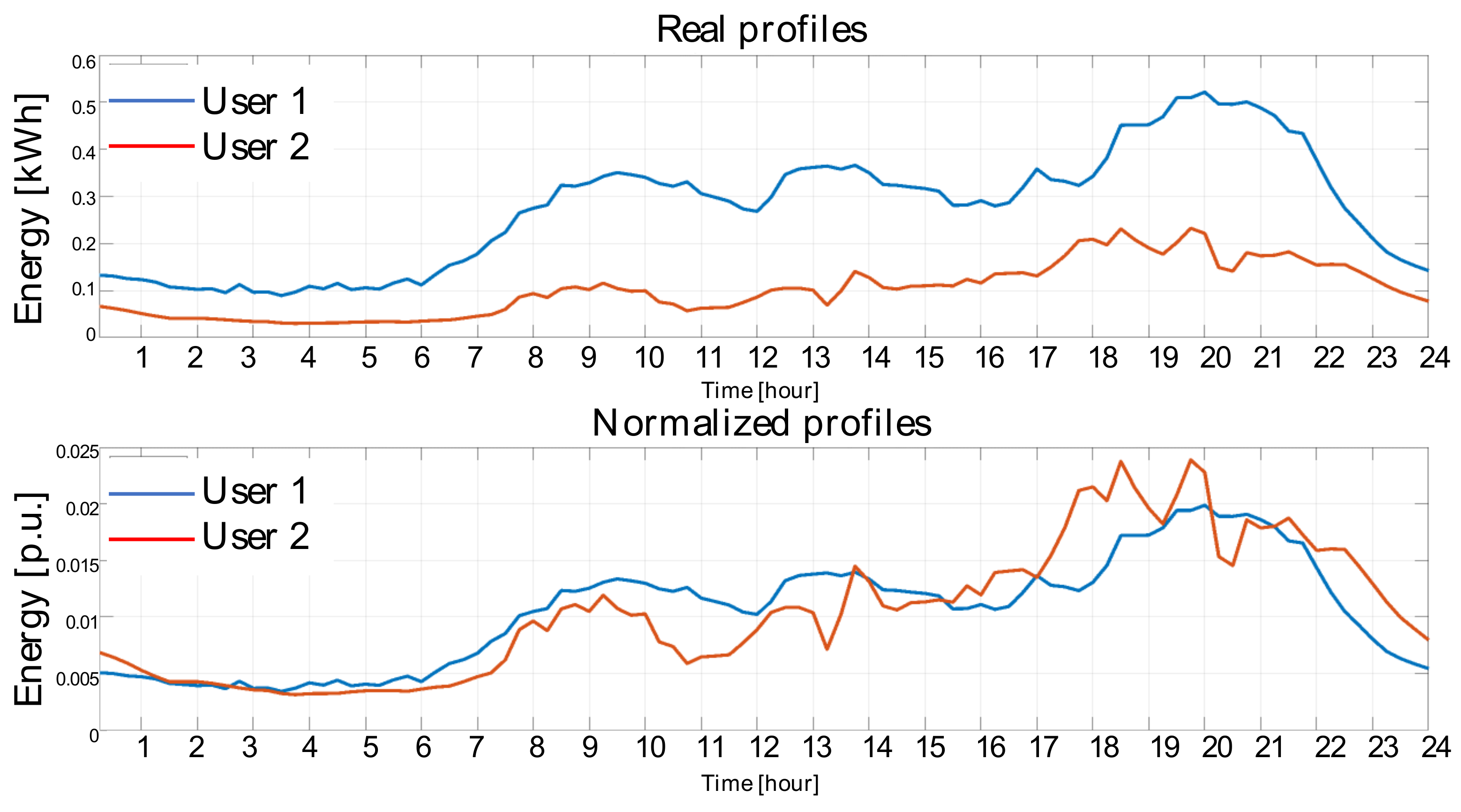
The customer characterization for each considered typical day group of daily load patterns is passed through normalization and PCA.

The normalization of the profiles is made by using the daily energy consumption. By considering the samples $s\left(t\right)$, for t = 1 … 96, of each daily profile $S$, the samples of the normalized time series $s_n\left(t\right)$ are calculated as in Equation (1).

$$s_n\left(t\right)=\frac{s\left(t\right)}{{\sum }_{h=1}^{96}s\left(h\right)}$$

(1)

where ${\sum }_{h=1}^{96}s\left(h\right)$ is the daily energy consumption. With this transformation, the sum of the samples of the normalized profiles is always unitary. This normalization makes customers’ profiles comparable even if they show different consumption levels, as shown in Figure 4.

In terms of the large number of profiles to be treated, before the clustering step, for reducing the dimension of the space of the features and, as a consequence, decreasing the computational effort of this stage of clustering, the PCA to the consumption pattern of 96 samples for each of the 12 typical days of the year is applied. The final selected features are the first p principal components that assure the decomposition covers a high percentage (e.g., >80%) of the variance of the original ones [30].

Once passed through the normalization and the PCA, the data are ready for the second stage of classification.

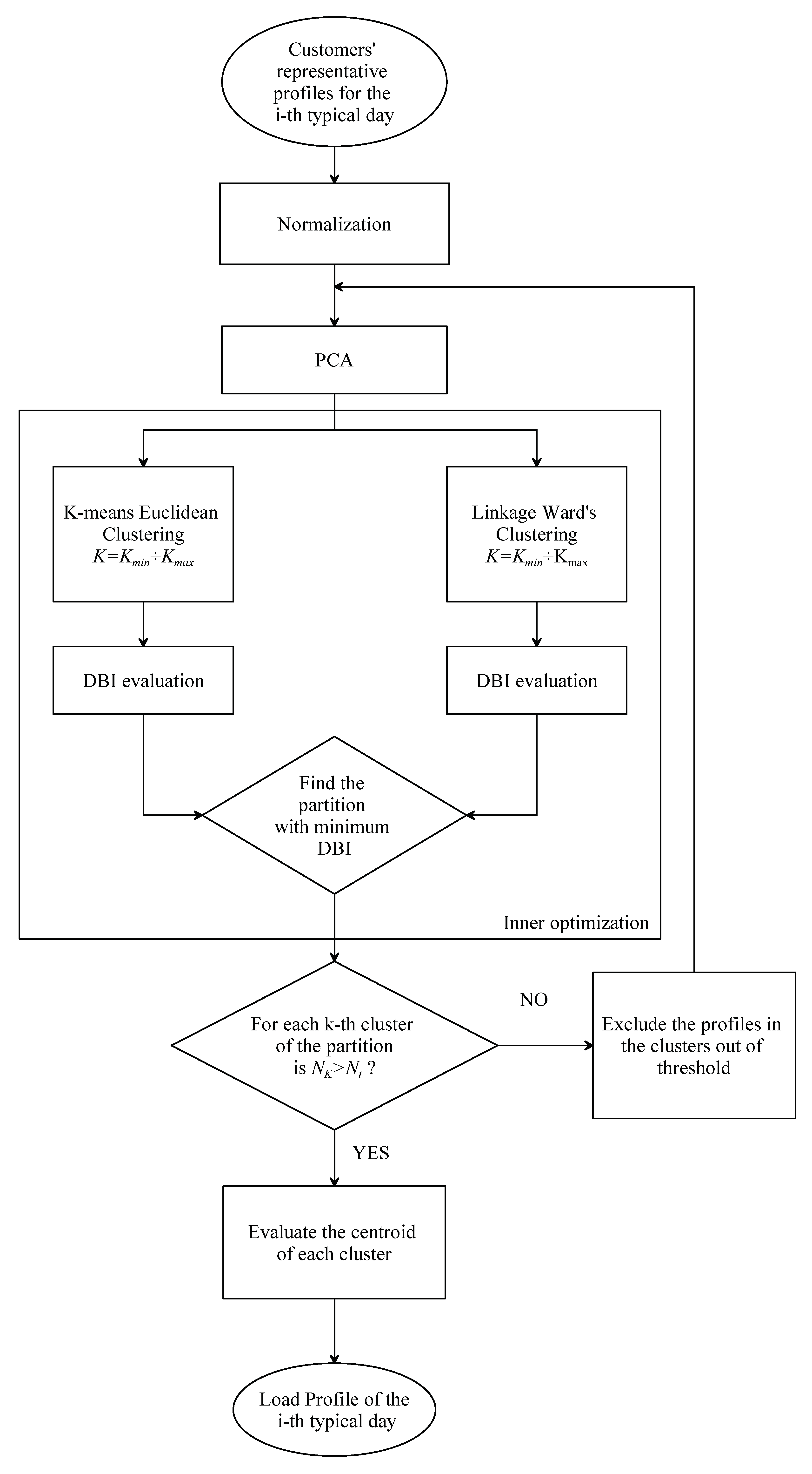
This stage is devoted to homogeneous grouping customers into classes by looking for the similarity of their consumption profiles’ shape Figure 5 shows the flow diagram of the proposed clustering approach that includes an inner optimization for defining the optimal number of clusters. Two clustering techniques, k-means and Ward’s hierarchical method, both with Euclidean distance as similarity metric, are compared for finding the most effective result. To objectively assess the reliability of the obtained partition, authors have proposed several clustering validity indices in the literature [10,28]. Among the most acknowledged validity indices (e.g., Davies–Bouldin [36], the Calinski–Harabasz [37], and the Silhouette index [38]), DBI is used in this paper for comparing the performance of the two clustering techniques. This index measures the level of separation among clusters. Moreover, since both the two clustering methods work with a priori defined minimum and maximum number of clusters (i.e., K_min, K_max), the clustering analysis is iteratively performed with both the two methods, by considering all the number of clusters in the a priori defined range. For each number of clusters in the range, the relevant DBI is calculated, with the final subdivision being the one that maximizes the performance (i.e., the DBI minimum value of among all the examined cases).

Furthermore, since the used clustering methods tend to maintain the clusters populated in a relatively uniform way, with a low attitude to isolate the outliers [28], an external iterative procedure is triggered to eliminate possible outliers. Suppose a cluster includes N_K customer profiles, with N_K lower than the defined threshold (N_t), the corresponding customers are excluded, and a new clustering analysis is performed on the reduced dataset. The process results are the centroids of the clusters relevant to each homogeneous group of customers. Each centroid represents the LP of the customers that belong to the cluster. It will also represent other customers with characteristics similar to the ones belonging to the corresponding cluster.

3.4. New Customers/Cluster Association

The procedure’s goal is to associate an appropriate consumption profile to new customers that cannot be characterized by a historical behavior (lateral path in Figure 1). The clusters obtained with the previous classification are analyzed to identify the features common to all members of the clusters. In this way, each cluster is identified with a small number of features that can be used to associate the cluster with a new customer. These features must be stored in the DSO’s customer database and be minimal to make their use as easy as possible. Annual energy consumption, geographic area of the customers, and peak hours are examples of features that can be used. Only features that are not used in the preliminary dataset segmentation can be used for this task. For instance, if the customers have been preliminarily subdivided using the geographic area they belong to, this information is useful for identifying the corresponding set of representative clusters. Still, it cannot be used for the association of a new customer.

Several features can be tested for characterizing the cluster. The first one is related to the climate. For instance, in Italy, the Italian national territory classification in climatic zones may be used. A “climatic zone” is identified by one of the first six capital letters (A–F) that attribute to each Italian municipality typical climatic characteristics [39]. A second feature is annual energy, particularly important for residential customers because it can be related to exogenous variables, such as the number of appliances and the annual salary. Other features are the seasonal or monthly peak values of the real profiles or of the centroid of clusters. Other tested features may be the geographic information, as region, province, and municipality, but if the available database does not uniformly cover the territory of interest (e.g., some regions are more represented than other ones), these features cannot be very useful for characterizing the clusters. Any other feature that the DSO could easily know should be evaluated to make this association the most reliable as possible.

However, once a limited number of features characterizes each cluster, the values assumed by such features drive the association of a new customer to the representative LPs. In this paper, the LP attribution is performed with two different goals:

• representing a single customer (new or existing but not monitored);
• representing a group of customers fed by the same secondary substation.

For the first goal, the association is performed by assigning a score to each obtained cluster. The score is based on comparing the value of the feature for the specific customer and the value of the same feature calculated for each cluster. For instance, let us assume that the selected feature is the annual energy consumption. The customer’s annual energy consumption is compared with the mean annual energy of the customers belonging to each cluster. The cluster that gains a score of 1 is the only one with the minimum distance. The other clusters gain 0 as a score for this feature. By repeating this counting for the variable number of the selected features, the cluster with the greatest score can finally be associated with the customer.

For the second goal, a simplified method for associating an LP to one group of customers is developed. The combinations of the annual energy of the customers (calculated or estimated) and their geographic location are used for identifying groups of customers (e.g., the northern customers with a yearly consumption in the range 1500 kWh/year $÷$ 2000 kWh/year). Thus, each cluster is characterized by the share of customers’ groups used to guide the association of customers and LPs. For defining the share of the i-th group of customers in each k-th cluster, the distribution coefficients $q_{ik}$ are calculated as in Equation (2).

$$q_{ik} = \frac{F_{ik}/N_k}{{\sum }_{j = 1}^C\frac{F_{ij}}{N_j}}$$

(2)

where $q_{ik}$ represents the distribution coefficient of the i-th group of users on the k-th cluster, $F_{ik}$ is the number of customers of the i-th group included in the k-th cluster, $N_k$ is the total number of customers in the k-th cluster, and $C$ is the number of resulting clusters. The ratio in Equation (2) considers the relative occurrence of the i-th group in the cluster k-th (in the numerator) and the same group’s cumulative occurrence in all the clusters.

The procedure for assigning LPs to customers whose daily profile is not known is based on defined distribution coefficients—consider a generic set U composed of n users of the generic group G. The users of the set are randomly distributed among the clusters according to the partition coefficients defined for the group G. At the end of the association process, the n users of the set U will be distributed over the clusters in a number proportional to the value of the corresponding partition coefficients. The LP associated with each user corresponds to the denormalized LP, i.e., the centroid of the cluster to which they have been associated.

4. Results and Discussion

The proposed approach was applied to two databases. The preliminary segmentation of the databases subdivided the customers on the basis of the type of contract and economic sector (i.e., main or secondary residence among the residential contract, and commercial, industrial, and agricultural among the other usage contract). Furthermore, each typical day (i.e., the 12 typical days differentiated by season and by workdays, Saturdays, and holidays) is handled independently.

Table 1. Parameters useful for the characterization of the single customer (first stage).

Parameter	Value
Maximum number of missing samples in a daily profile (the percentage of the number of intervals on which the day is discretized, i.e., 96 intervals of 15 min each)	25% (24 samples/day)
Minimum number of “valid” typical day profiles to be suitably represented	7 (weekdays), 4 (Saturdays and holidays)
Methodology for assessing the typical daily profile of a given customer (for customers suitably represented)	most frequent average profile
Methodology for assessing the typical daily profile of a given customer (for customers not suitably represented)	average profile
Normalization (yes/no)	no
Used clustering algorithm	Ward’s agglomerative
Minimum (Kmin) and maximum (Kmax) number of clusters examined—weekdays	2$÷$6
Minimum (Kmin) and maximum (Kmax) number of clusters examined—Saturdays and holidays	2$÷$3
Similarity: minimum number of profiles included in the most crowded cluster	60%

and

Table 2. Parameters useful for grouping customers into classes (second stage).

Parameter	Value
The threshold of daily energy consumption	0.6 kWh/day
Mean and standard deviation limit (${\mu }_{lim}$ and ${\sigma }_{lim}$)	10% of μtot and σtot
Decomposition covered by the principal components (PCA)	80% of the variance of the original data
The threshold for excluding cluster with a few customers (Nt)	10% of the input customers
Normalization (yes/no)	yes
Used clustering algorithms	k-means and Ward’s agglomerative
Minimum (Kmin) and maximum (Kmax) number of clusters examined	3$÷$6

report some parameters used to characterize a single customer (first stage of the classification process) and grouping customers into classes (second stage of the classification process), respectively.

A single customer’s characterization was applied only to the customers that did not change the type of contract within a season. A given typical day’s active power patterns are constituted by enough samples (i.e., greater than the maximum number of missing samples). According to this rule, one customer could be possibly analyzed for one season only (i.e., three “valid” typical days). The methodology used for finding the customer’s representative profiles may vary if the customer is suitably represented or not. In particular, if there are more than the minimum number “valid” typical days, the most frequent average profiles (according the method described in Section 3.3.1 was used, otherwise the mean value of the corresponding 15 min samples of all the days of the same type in the year was calculated. Since the adopted clustering techniques are both vised, a minimum (K_min) and maximum (K_max) number of clusters to be examined have been considered. Finally, a comparison between resulting clusters was performed for aggregating clusters that exhibited a certain degree of similarity. This task’s similarity index was based on the correlation coefficients assessed by assuming a defined probability distribution (i.e., T-student distribution, with alpha = 0.1). The stop criterium in the aggregation process was reached when the most crowded cluster included more than a minimum number of daily input profiles (as the percentage of the number of valid days).

Starting from each customer’s representative profiles, the second stage of the classification process followed the procedure described in Section 3.3.2 applied to further selected groups of profiles. The further selection aimed at eliminating the outliers, i.e., the daily profiles with an energy consumption smaller than a significant threshold or too flat (i.e., with mean ${\mu }_d$ and standard deviation ${\sigma }_d$ much smaller than the limit parameters, ${\mu }_{tot}$ and ${\sigma }_{tot}$, calculated for the totality of the profiles). Table 2 also reports other information about the rules for excluding clusters too poorly crowded (according to the flow chart in Figure 5), etc.

4.1. Databases

Two databases (DBs) were used in this paper. They were constituted by the consumption patterns of tens of thousands of Italian customers acquired with a sampling rate of 15 min for two measurement campaigns conducted in different years (i.e., between the years 2013 and 2014, hereinafter referred to as DB2013, and in 2017, referred as DB2017), and by two registers with some information about the customers. For each customer included in the registers, several features were known, not all significant for this study:

• type of contract (i.e., main or secondary residence contracts, or “other usage” for customers different from residential);
• the economic sector, useful for distinguishing customers different from residential into the traditional categories (i.e., industrial, commercial, and agricultural);
• prosumer or not, and in the case of yes, the rated power of the generation plant;
• rated power (e.g., the typical rated power of residential customers is 3 kW);
• the phase of the connection (only for the 2017 database);
• geographic information (i.e., region, province, municipalities), useful for associating the climatic zone (identified by one of the first six capital letters (A–F), univocally identified by the municipality [39]);
• monthly energy consumption (kWh/month), useful for assessing the yearly energy consumption (kWh/year).

It is worth noticing that the measured consumption profiles and the register of the customers included in the databases were not homogeneous, even if they referred to the same year’s dataset. Furthermore, even for the customers included both in the registers and in the profiles’ database, the data were not always reliable. For instance, in many cases, several monthly consumption patterns were missing for a specific customer. Thus, his/her yearly consumption cannot be exactly calculated but, in some cases, only reasonably estimated. Therefore, many customers were excluded from the study due to incompleteness (i.e., too many null samples or no commodity sector/type of contract identification). The empirical rules defined according to the setting parameters reported in Table 1 were applied to pre-process the data and limit the study to sufficiently reliable and accurate data. After the pre-selection, the share of the final groups of customers established to be valid for the next analysis was assessed. Moreover, further selection operated during the second stage of the classification process for eliminating the outliers reduces these shares (Table 2). In

Table 3. Share of valid customers/final number of customers clustered (outliers excluded) in the two considered databases.

Database (Year)	Main Residence	Secondary Residence	Agricultural	Commercial	Industrial
2013	41,289/38,928	4577/4577	182/180	8963/8937	1023/1023
2017	24,453/22,838	2532/2527	112/112	3537/3533	1156/1145

the maximum number of valid customers of each category and the resulting maximum number of clustered customers of each category among the seasons are reported, differentiated for the two available databases. Since the selection of valid profiles considerably reduced the initial number of customers included in the databases, and the final number of analyzed customers may vary from one season to another, in this study, in order to maximize the size of samples for each season, all the profiles that pass the pre-processing stage for the single season are used. From the data in Table 3 it can be seen that the outliers eliminated by the iterative procedure described above were very few in number. The percentage of reduction reached a maximum of 6.6% (i.e., in the residential customers with a main residence contract in the 2017 database).

Unfortunately, the number of prosumers is very limited in the two databases—only a few hundred customers were prosumers. Thus, despite the importance of this category of LV customers, they are disregarded in the performed analysis.

4.2. Resulting in Typical Load Profiles

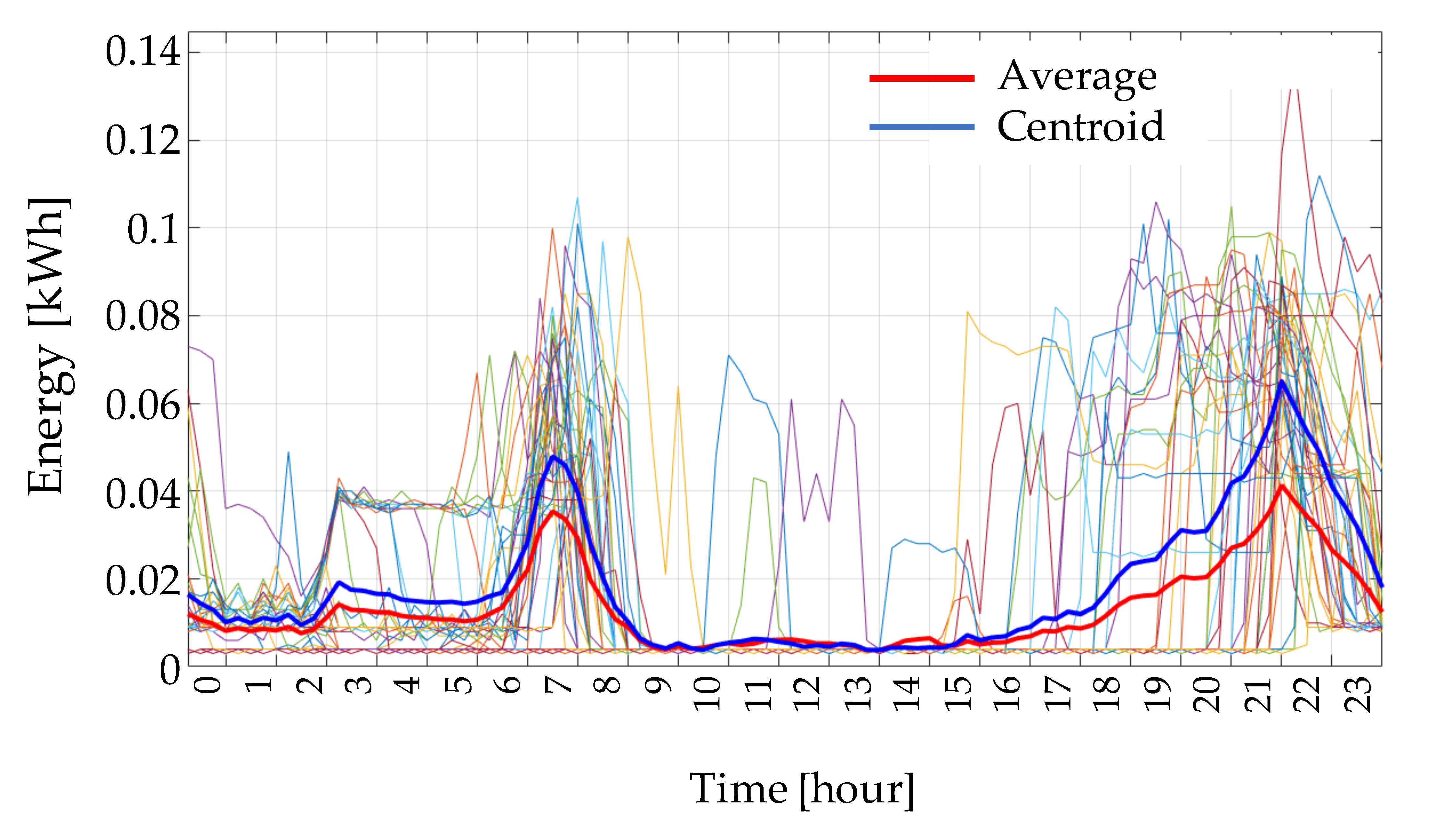
The result of the single customer’s characterization process is graphically shown in Figure 6 wherein the real consumption profiles of a given customer on winter workdays are drawn. The variability of consumption in winter weekdays causes the aggregation into three clusters represented by their relevant centroids. In Figure 7 the most crowded cluster in Figure 6 is zoomed in for showing the difference between the centroid (blue line), which can be used to represent that customer in that quarter of the year, and the average profile (red line), obtained by averaging all the real profiles of Figure 6. The average profile tends to flat the valleys in the early hours of the day and reduce morning and evening peaks.

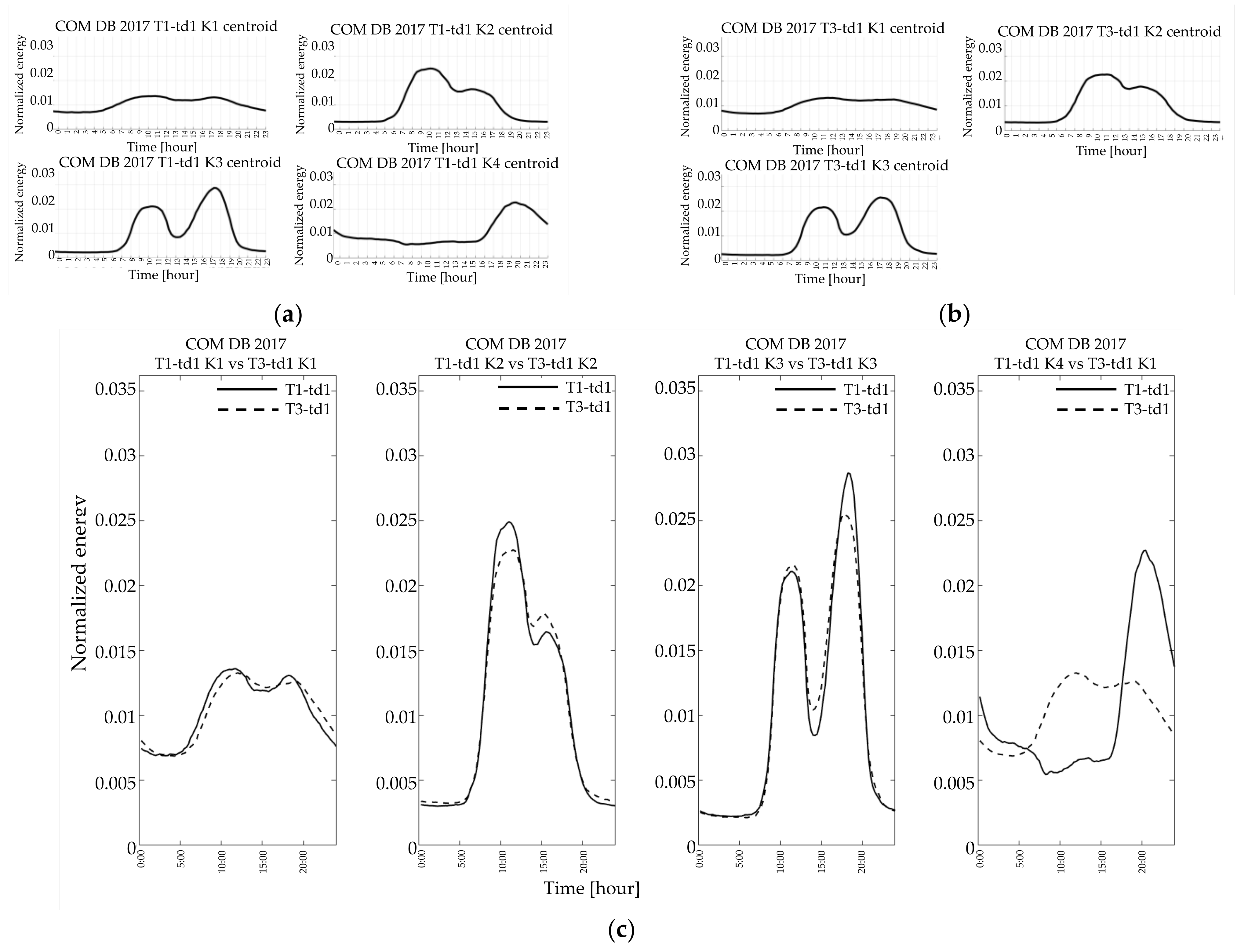
In the following section, for the sake of brevity, the description and discussion of the results focus on three categories of customers (i.e., commercial, industrial, and main residence contract) and two typical days, one in winter and one in summer (i.e., the working days of the first and third quarter. Figure 8, Figure 9, Figure 10, Figure 11, Figure 12, Figure 13, Figure 14, Figure 15 and Figure 16 show the two databases’ resulting centroids, DB2013, and DB2017. The resulting clusters are in descending order, from the largest to the smallest. Furthermore, the comparison between seasons within the same year, and, finally, the comparison between years, for the three categories of customers, are reported. The comparison considers the most similar normalized profiles besides the crowdedness of each cluster with a calculation of the minimum root sum square error:

• The number of resulting clusters may vary from season to season both in DB2013 (i.e., Figure 8a,b, and Figure 14a,b) and in DB2017 (i.e., Figure 9a,b and Figure 15a,b) for commercial customers and residential ones; this did not happen for the industrial customers (Figure 11a,b and Figure 12a,b).
• The profiles of the two typical days during the two seasons can be similar, as shown in Figure 8c, Figure 9c, Figure 11c, Figure 12c, Figure 14c, Figure 15c, even if in some cases the peaks can be slightly moved or reduced.
• Profiles of different years can be almost overlapped (i.e., Figure 10a, Figure 13 and Figure 16).
• In some cases, the two-year comparison makes very similar shapes but higher/lower peak values in the two DBs (i.e., Figure 10b).

The commercial customers (Figure 8, Figure 9 and Figure 10) exhibited profiles of typical days of the same year quite similar in shape (e.g., Figure 8a,b and Figure 9a,b), demonstrating that customers other than residential exhibit less variability than residential customers even during different days of the same year. Furthermore, by comparing the shapes resulting from the clustering of different years, some similarities occur, both in the winter (Figure 10a) and in the summer working days (Figure 10b).

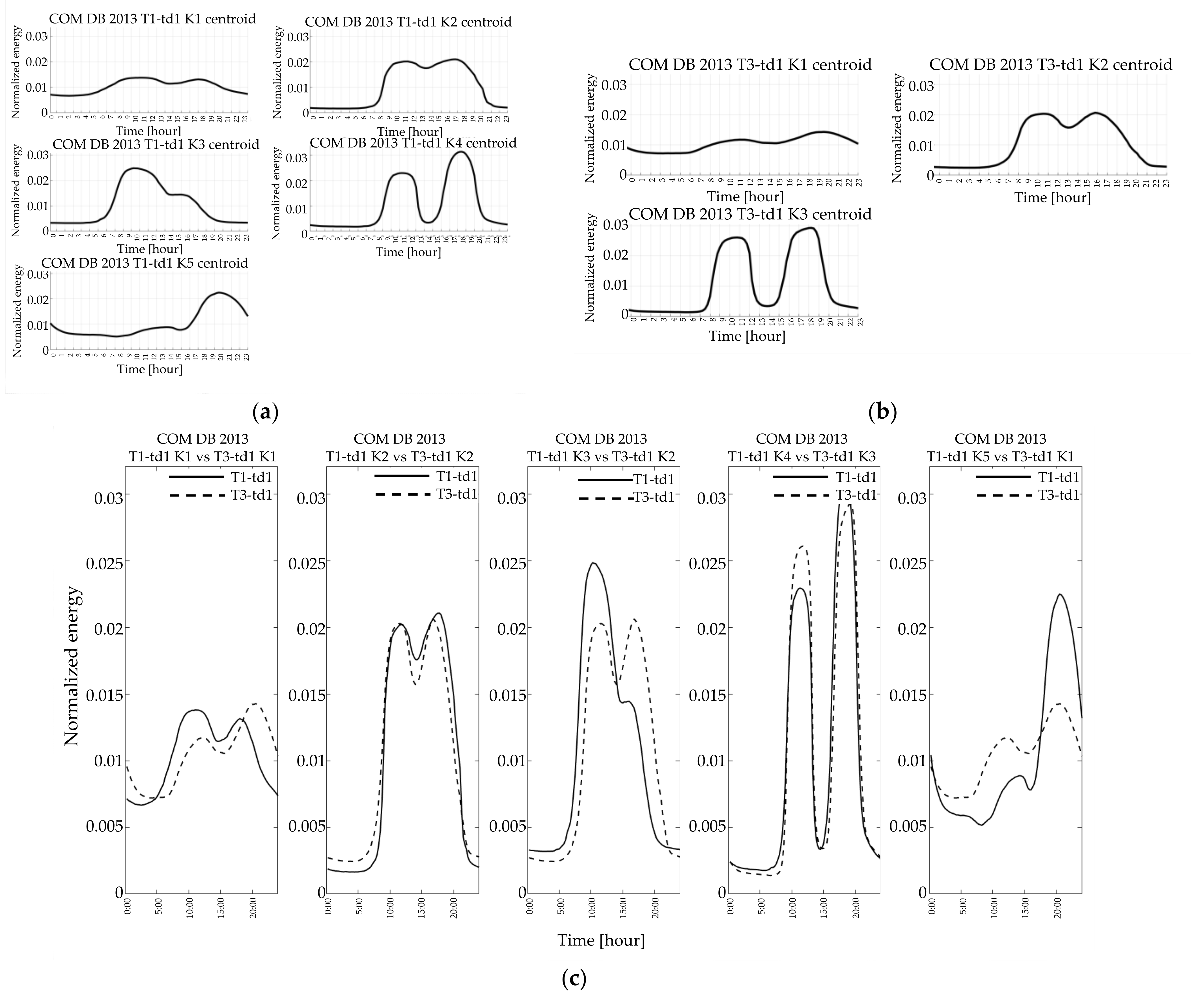
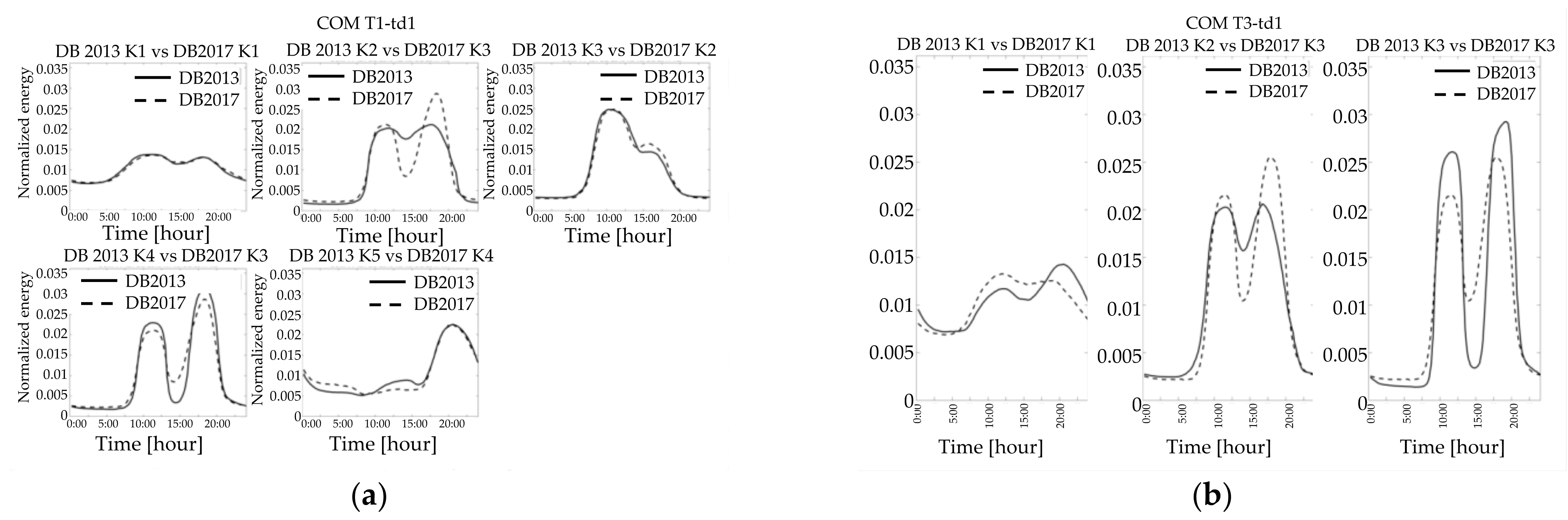
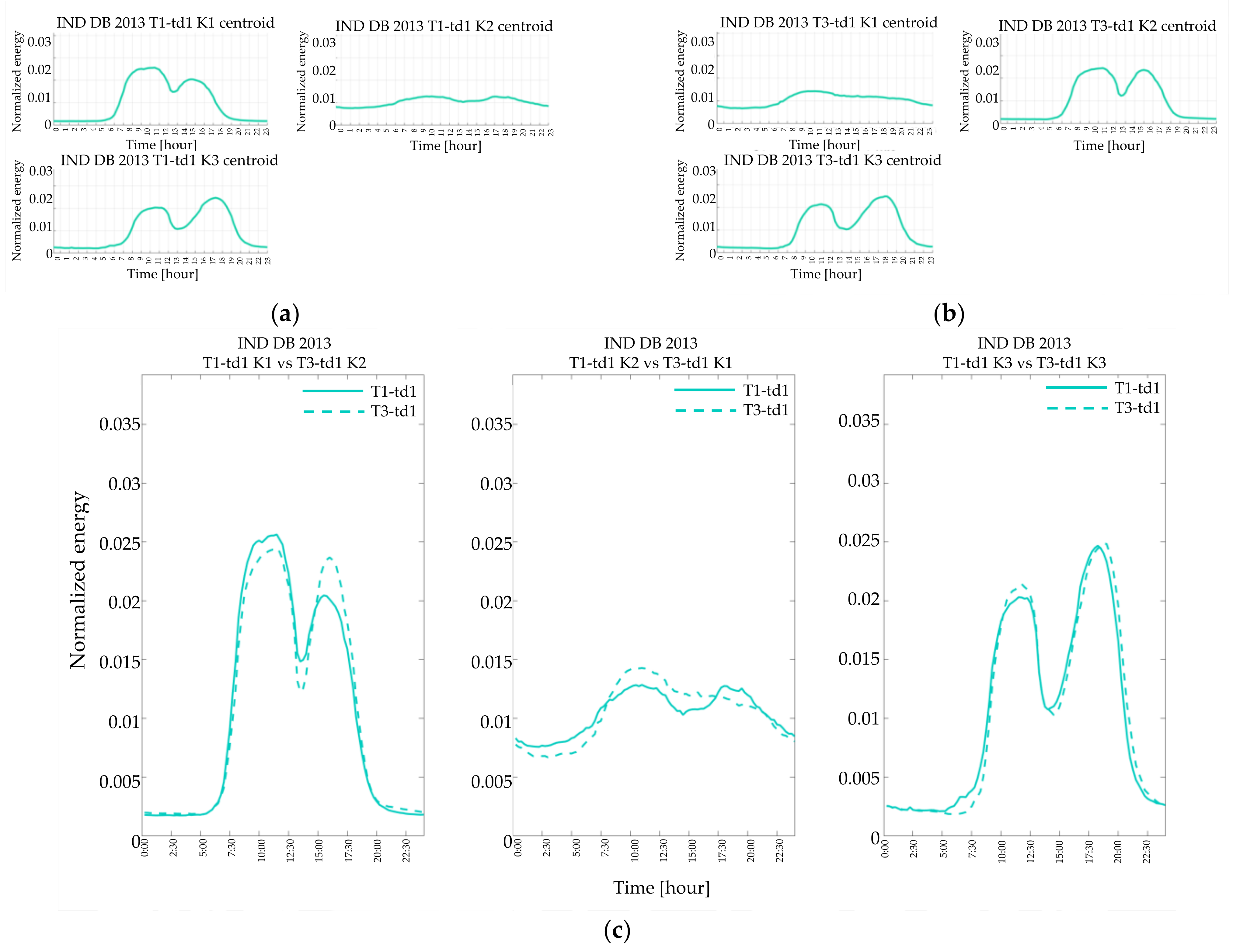
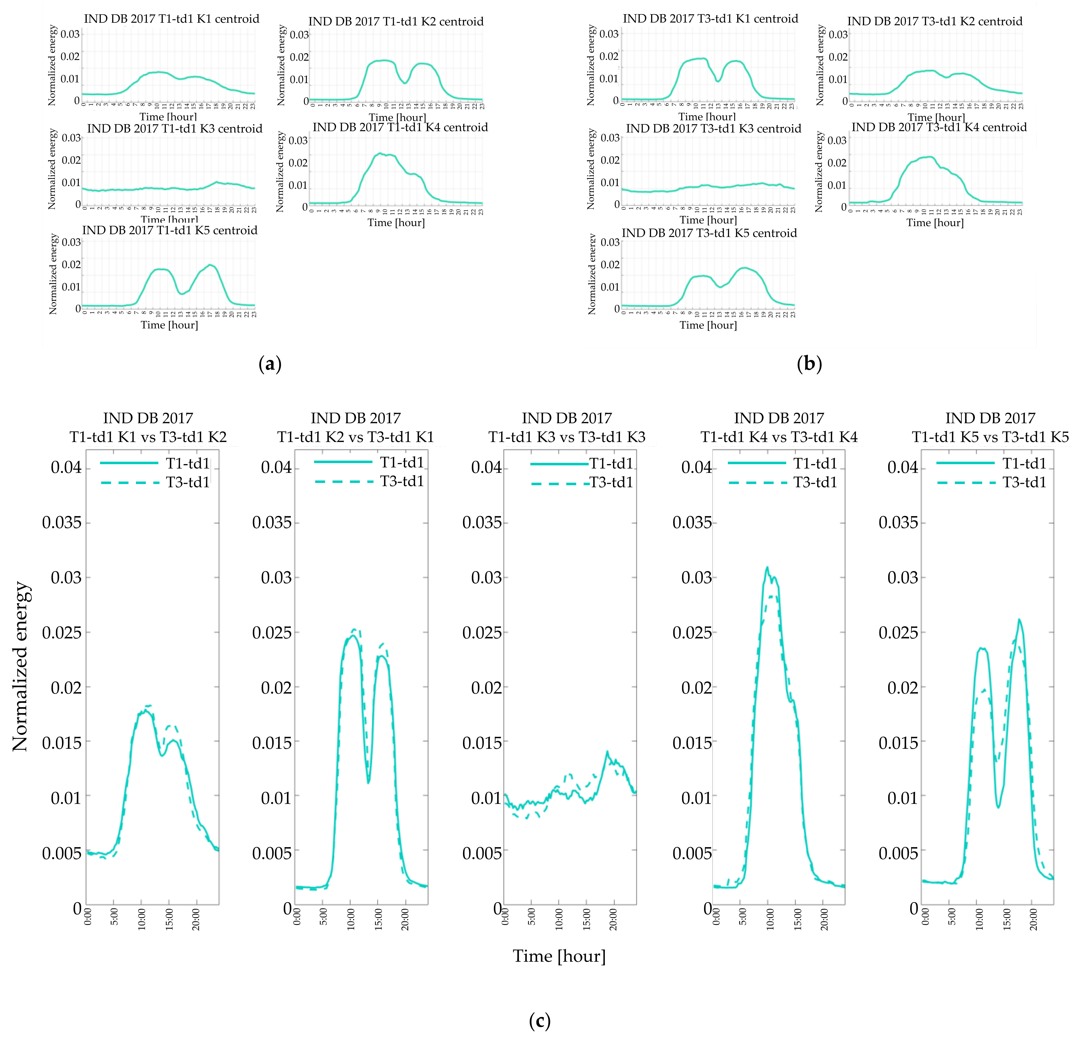
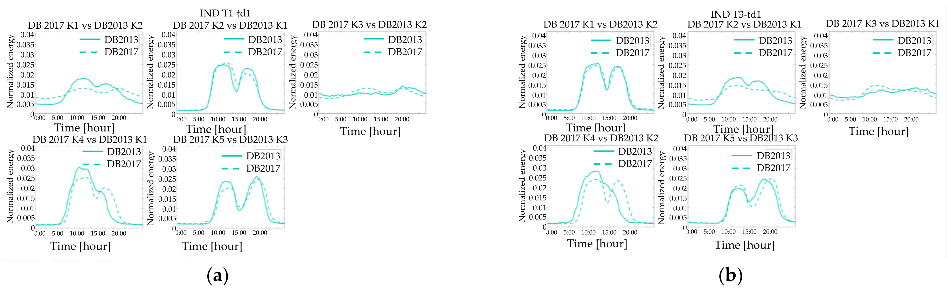
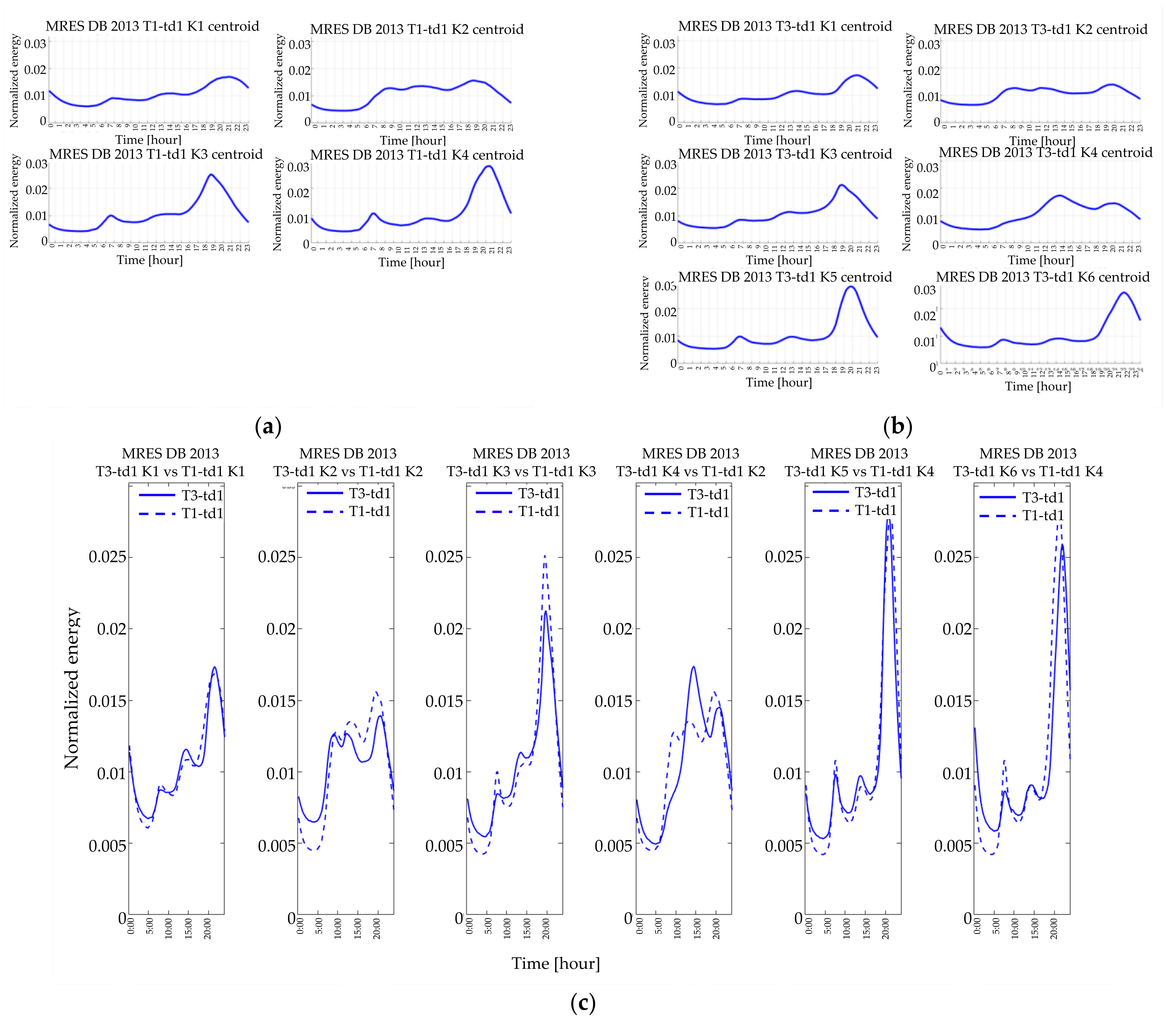
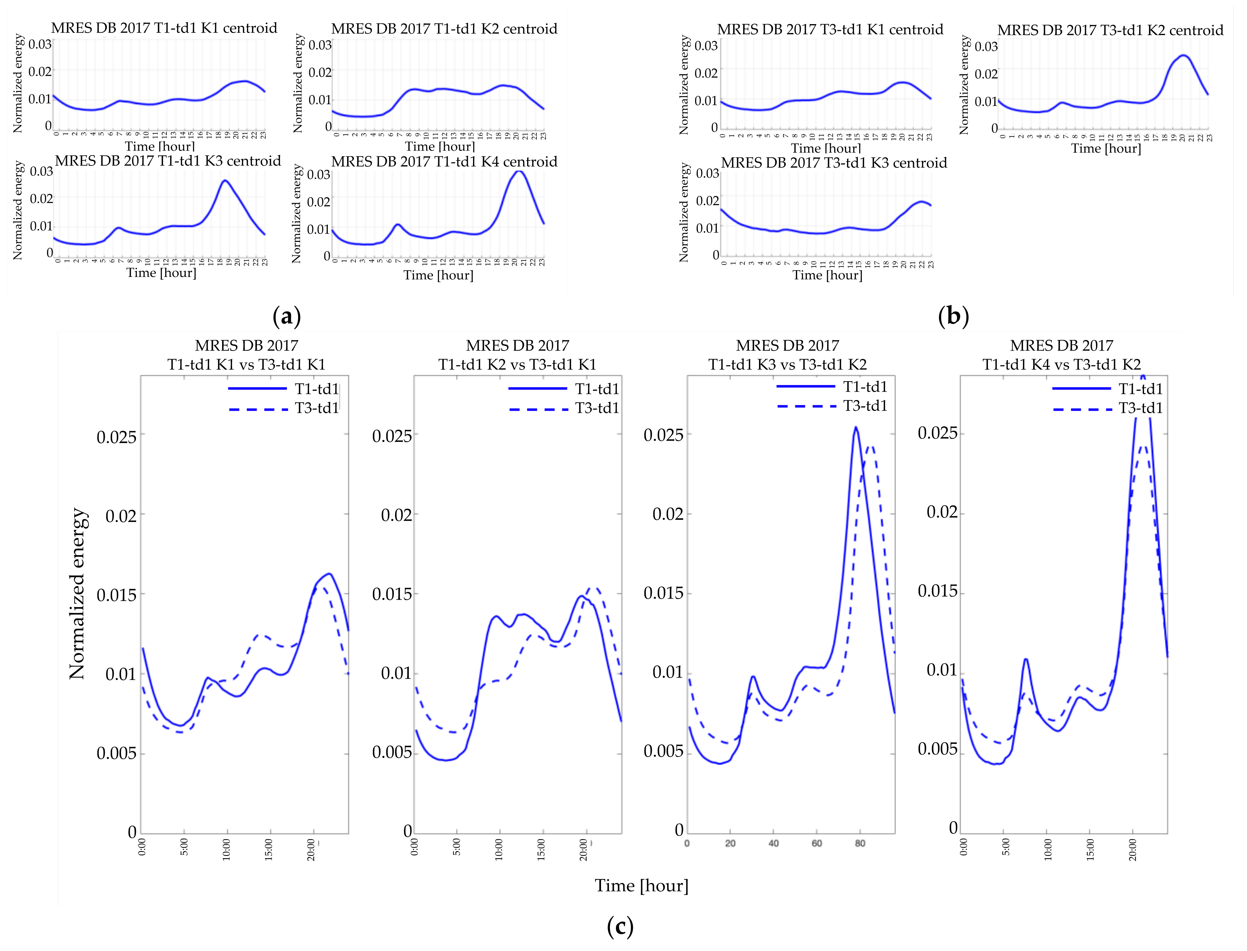
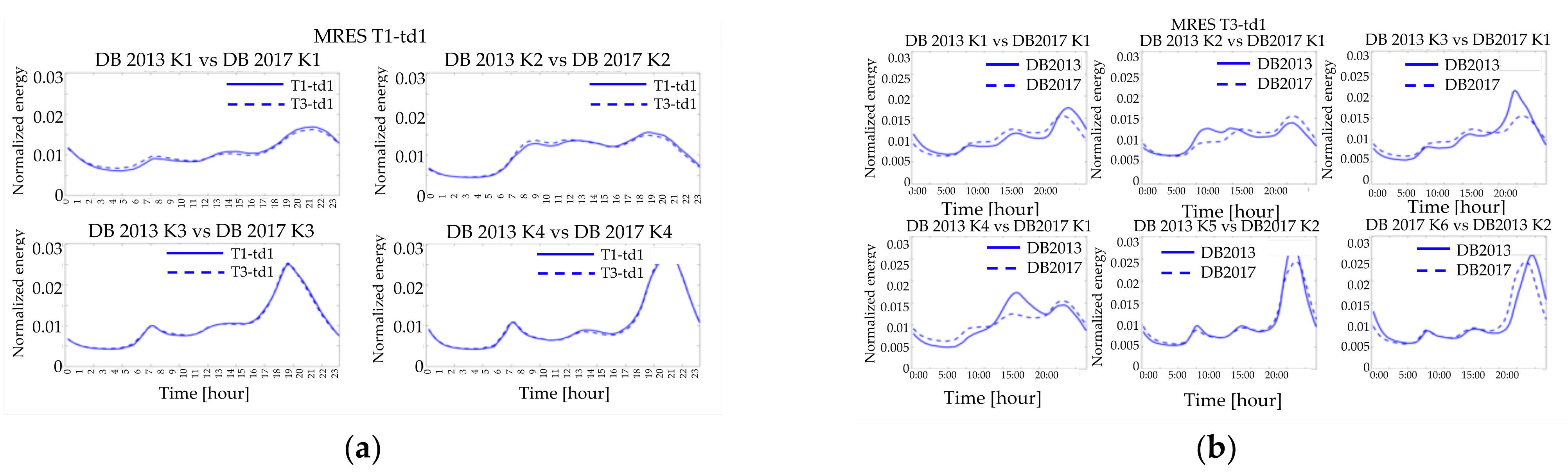
Regarding the industrial customers, the similarities between profiles of the same year (Figure 11c and Figure 12c) are even more evident than for the commercial customers. Moreover, the number of resulting clusters is the same in the two seasons considered. By comparing the two different years, it can be found that, although there can be a reasonably perfect correspondence between centroids of the two databases (e.g., K2 of DB2013 is very similar to the K5 of the DB2017), it may occur that one shape can be considered similar to two of a different year (e.g., the centroid of the cluster K2 of the DB2013 is similar to both the DB2017 centroids of K1 and K3 in the typical winter day and of K1 and K4 in the typical summer day, as seen in Figure 13a,b).

Finally, although for the residential customers the comparison between the days of different seasons points out significant differences (i.e., Figure 14c and Figure 15c), it should be recognized that the comparison of typical homologous days shows a correspondence in the examined years (Figure 16a,b). In particular, the winter workdays’ LPs are almost the same, and there are a reasonably perfect coincidence between each shape in terms of peaks and valleys (Figure 14a and Figure 15a). The only difference is in the cluster sizes because the first two clusters’ order is switched in the DB2017.

4.3. LP Attribution

Once LPs representative of a given group of customers are identified, the analysis of the characteristics of the customers belonging to each cluster allows for the identification of a set of features that justify the existence of the clusters. These features are used to find a proper LP for customers not in the DSO customers’ database due to the absence of smart meters or their novelty. LPs’ attribution to existing but unmonitored customers can be used to assess the operating conditions of the network components (i.e., lines and transformers), calculate the power losses, and determine the expected voltage profile.

The association starts with the analysis of the customers in each cluster to find common features such as

• geographical (e.g., municipality, region, or altitude, etc.);
• electrical, related to the contract or the consumption (e.g., rated power, or annual energy, etc.);
• inherent to the shape of the profiles (e.g., monthly or season peaks, the hour of the day of the peak or the valley).

Many tests were performed, and as a result, only a few features were proven to be effective for some customer categories for the databases studied in this paper. The chosen few features were the annual energy (subdivided in quarterly energy, for considering each season separately) and the monthly or seasonal peak values, easily known by the DSO for each customer. These features were modeled as normally distributed random variables in the cluster. Thus median, mean, and standard deviation were calculated for each feature.

Cluster features are the input of the scoring method used for choosing the suitable LPs for a new single customer, according to the procedure described in Section 3.4 The accuracy of the proposed method was evaluated with a simple process. Each customer was associated with the cluster with the maximum score. The percentages of the right customer/cluster associations for the 2017 database are reported in

Table 4. Number of the right customer/cluster associations for the customer included in the DB2017.

Type of Contract	T1-td1	T1-td2	T1-td3	T2-td1	T2-td2	T2-td3	T3-td1	T3-td2	T3-td3	T4-td1	T4-td2	T4-td3
Main residence	31.0%	30.1%	26.8%	51.5%	60.9%	48.3%	71.8%	71.0%	62.9%	51.0%	36.0%	33.4%
Secondary residence	39.7%	35.1%	31.0%	37.6%	25.4%	28.1%	44.4%	44.5%	40.6%	38.2%	25.0%	18.6%
COM	43.8%	50.0%	59.1%	52.5%	57.6%	66.4%	50.7%	50.1%	66.0%	47.3%	48.3%	63.1%
IND	36.2%	31.1%	76.0%	41.7%	47.0%	72.5%	37.3%	28.6%	67.6%	43.2%	39.3%	64.1%
AGR	71.1%	63.6%	55.3%	72.9%	73.3%	75.0%	86.7%	83.7%	92.5%	84.8%	85.7%	86.7%

. In the table the color scale emphasizes the results: i.e., in each row the worst value is in dark blue and the best is in bright red.

The association to the right group succeeded in the range 26.8% ÷ 71.8% of the main residence customers depending on the typical day considered. For the other customer categories, the rate of success was similar. Although most of these results are encouraging, in some cases, the success rate was minimal (e.g., the minimum percentage of success was 18.6% for the autumn holiday, T4-td3). There are several reasons for this low success rate. The most significant reason is that the clusters’ features are not normally distributed for all the clusters, and their probability density function is far from a normal distribution. It is worth noticing that Gaussian approximation’s accuracy increases with the number of customers in the cluster and the feature’s correlation with the centroid shape.

For the representation of a group of customers fed by the same secondary substation, the available databases are split, referred to as the Italian territory, into 5 geographic areas (i.e., center, islands, northeast, northwest, south) and 17 ranges of quarterly consumption (the first range E₀ corresponds to consumption smaller than 50 kWh/year; the following are calculated according to the rules E_i-1 ≤ E_i < E_i-1 + 50 kWh/year; the last range E₁₆ ≥ 5000 kWh/year). By combining geographic areas and annual energy ranges, 85 groups of customers not all represented in the database can be identified. As an example,

Table 5. Customer shares in the cluster (F_ik) and distribution coefficients (q_ik) for the groups of customers of the northwest area (NW) in the four resulting clusters (database 2017).

Groups	Customer Share in the Clusters Fik				${\displaystyle {\displaystyle \sum }_{\mathit{j} = \mathbf{1}}^{\mathit{c}}}\frac{{\mathit{F}}_{\mathit{i}\mathit{j}}}{{\mathit{n}}_{\mathit{j}}}$	Distribution Coefficients qik
	K1	K2	K3	K4		K1	K2	K3	K4
NW-E0	12	14	14	3	0.07	0.29	0.27	0.32	0.11
NW-E1	95	126	89	57	0.65	0.26	0.27	0.23	0.24
NW-E2	133	205	144	80	0.98	0.24	0.29	0.25	0.23
NW-E3	116	150	151	93	0.92	0.22	0.23	0.27	0.28
NW-E4	92	108	112	75	0.70	0.23	0.21	0.27	0.29
NW-E5	117	105	87	53	0.64	0.32	0.23	0.23	0.23
NW-E6	9	5	1	1	0.03	0.58	0.26	0.06	0.10
NW-E7	1	1	1	1	0.01	0.23	0.19	0.22	0.36
Sum (Nk)	575	714	599	363

. reports the shares in the cluster (F_ik) and the distribution coefficients (q_ik) for the main residence contract customers of the northwest area in the four resulting clusters. Only 8 (i.e., E₀$÷$ E₇) among the 17 ranges of quarterly consumption are represented in the database. By analyzing the numbers in the table, one can see that the occurrence in the cluster K4 of a customer belonging to the group NW-E₇ gained greater importance than the one of a customer belonging to the group NW-E₆ because the group NW-E₇ is overall less numerous than the NW-E_6. For instance, a development plan that requires feeding about 100 customers, half belonging to the E₄ and the others to the E₅ group, can be studied by randomly associating the centroids of the four clusters to the customers according to the share of the coefficients in Table 5 (i.e., 16 E₅ customers will be represented by the centroid of the cluster K1, opportunely denormalized for taking into account the specific quarterly consumption).

5. Example of Application in Smart Grid Planning and Operation

For validating the whole approach, one example of application of the LPs is proposed in this section. It may be related both to the use of the LPs during the operation and the planning of the distribution system, since it compares the results obtained by performing load flow calculations of a given network. The comparison is made by varying the representation of the load demand: (i) by considering the measured load profiles, (ii) by using the LPs resulting from the approach proposed in this paper, and (iii) by assigning a unique set of LPs to each customer of a given category (according to the current DSO practice).

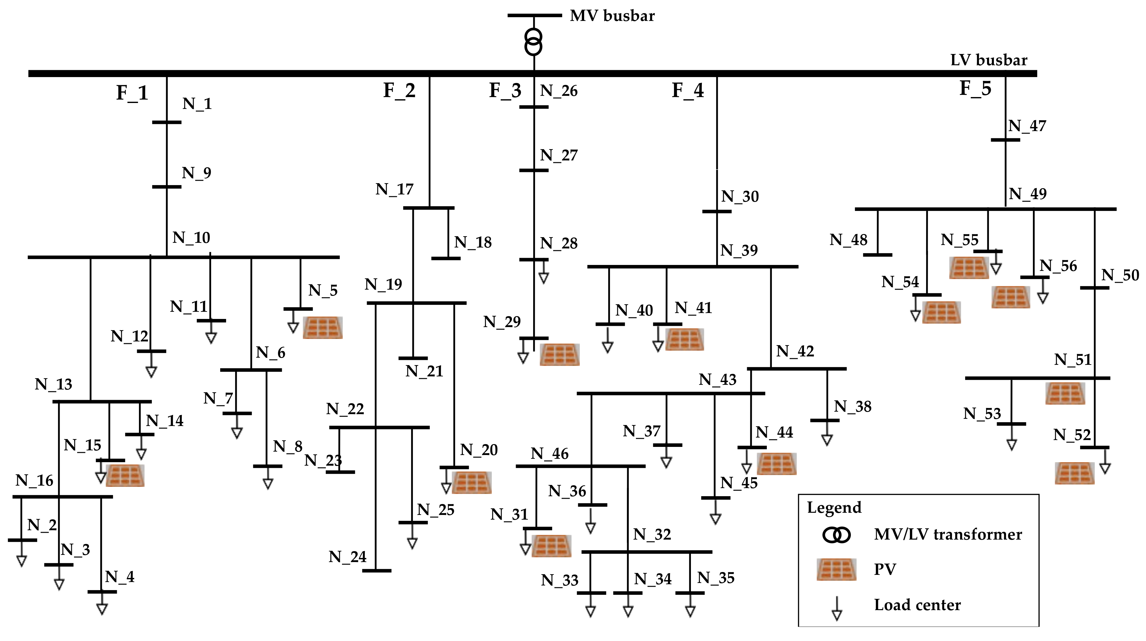
Figure 17 shows the LV network used for the test. It is constituted by 56 three-phase nodes distributed in five underground feeders and supplied by a 630 kVA MV/LV transformer and 27 photovoltaic generators (PV) located in 12 network nodes (i.e., single or three-phase, installed power from about 1 kWp and 62 kWp). The bulk grid and the PVs deliver energy to 516 residential customers (i.e., main residence contract, single-phase, rated power 3 kW) and 41 small or medium commercial customers (i.e., commercial contract, single or three-phase, rated power from 3 kW to 50 kW). For the sake of brevity, only the results for the winter working day are presented and discussed (i.e., first trimester), but this may come to the same conclusions for the others typical days.

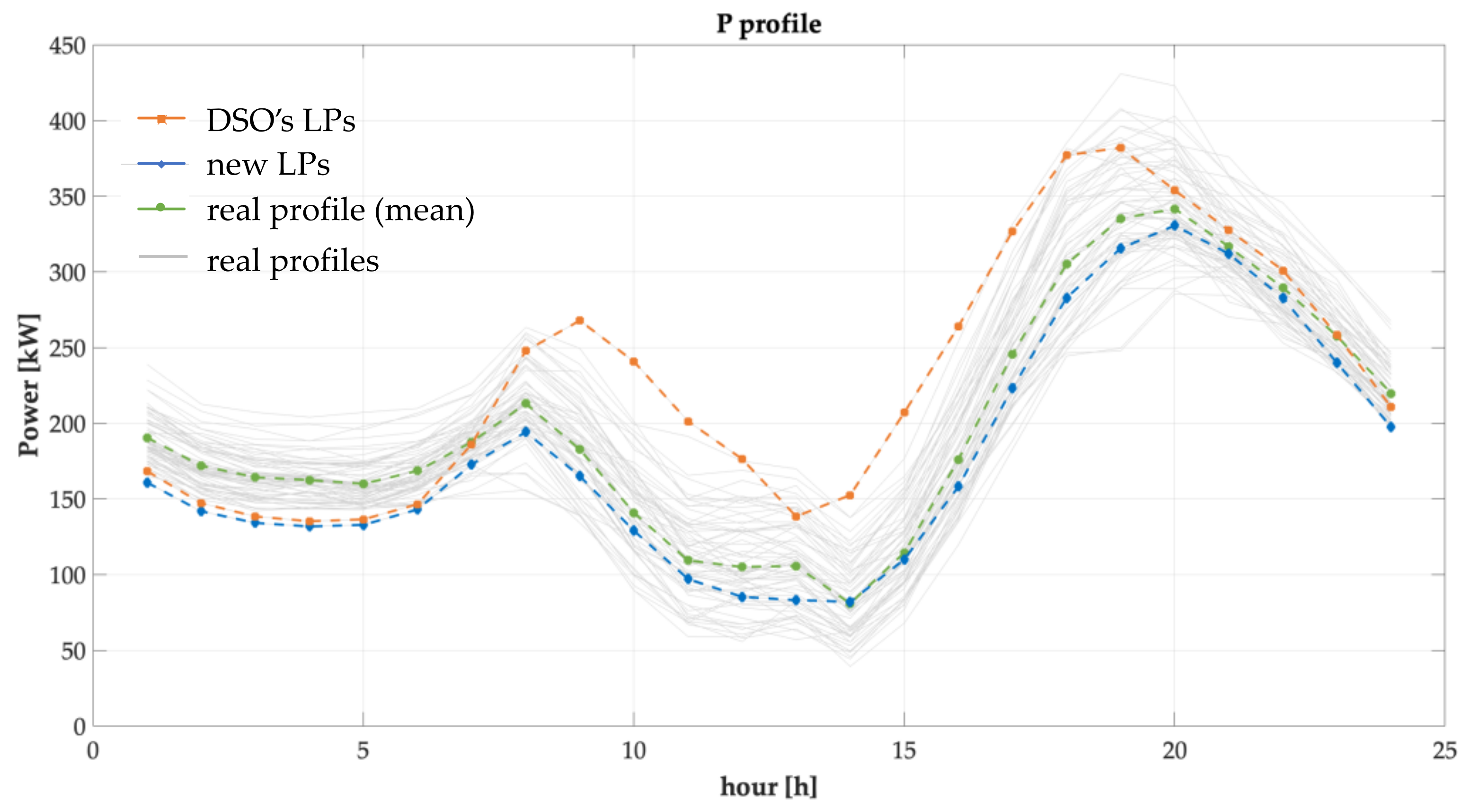
Figure 18 shows the power profiles at the MV/LV transformer calculated with the considered different set of typical load profiles and with the measured profiles. The real day power profiles of the about 65 winter working days of the year are reported in light grey, and their mean value is reported in green. The orange power profile refers to the use of the typical LPs currently adopted by DSOs. This curve highlights the effect of using the same typical LP for all the customers belonging to the same category. This use unavoidably overvalues the power profile in almost all the hours of the day and in particular ends up overestimating both the morning and the evening peak. Furthermore, the peak hours are delayed. On the contrary, the blue curve, related to the new typical LPs proposed in this paper, is very close to the mean real day power profile and guesses the peak hours.

Often, distribution management systems (DMS), by active managing the distribution networks, optimize one day ahead the scheduled generation/consumption patterns by forecasting the contingencies of the next day and by assessing the services that the DSO should procure possibly by the DERs. Obviously, the day ahead power/generation profile differs from real ones since forecast can never obtain no forecast error. Forecast errors on load consumption can be reduced if updated time series that properly represent the consumption and generation are used. Since in the real-time management of the network the goal is keeping voltage and power flows within the technical limits, the effectiveness of the approach can be furthermore validated by considering the resulting node voltage profiles. In the following, the analysis of the node voltages is focused on the feeder F_4. This feeder is the most critical one, for its length (it is about 400 m) and for the heavy load demand. For these reasons, such a feeder may suffer for excessive voltage drops in several hours of the day. 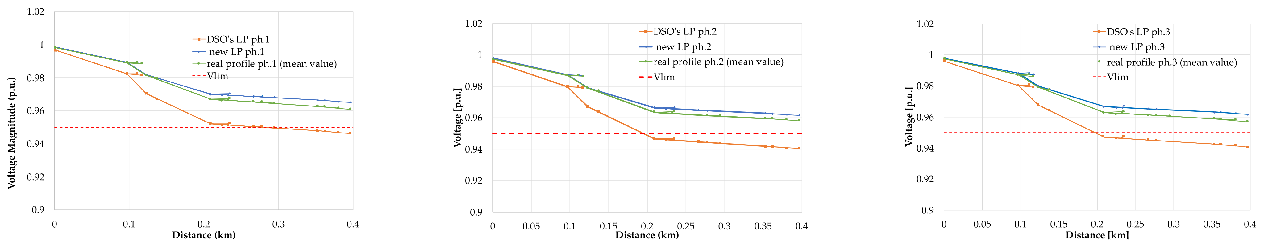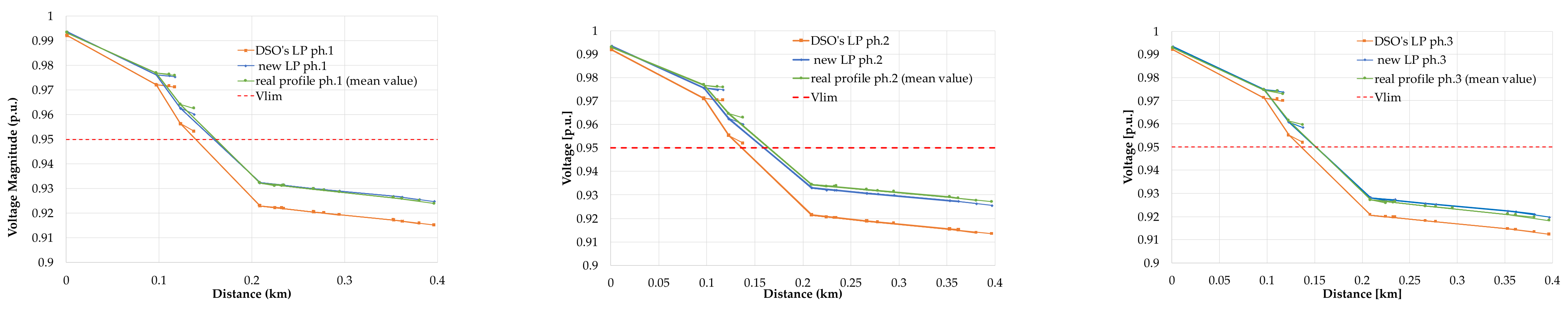Figure 19 and Figure 20 show the three-phase voltage profiles of the feeder F_4 at two hours of the winter working day (at 11:00 a.m. and at 6:00 p.m., respectively). The comparison is made by considering the mean value of the phase node voltages of the ≈65 real winter working days that occur in the year. The load supplied by the three phases is not balanced, and, thus, the voltage profiles of the three phases are not perfectly coincident. By these graphs, it is evident that the blue profiles (i.e., the ones derived by applying the new typical LPs proposed in this paper) are closer to the mean real day profiles (i.e., green profiles) than the ones obtained by LF calculations performed starting by the typical LPs currently adopted by the DSO (i.e., orange profiles). The overestimation of the power (see Figure 18) causes voltage drops more severe than the real case. Indeed, such behavior not only exacerbates critical conditions (e.g., as at 6:00 p.m., when severe under voltages occur even in the real case Figure 20), but also creates excessive voltage drops when they simply did not exist (i.e., at 11:00 a.m Figure 19). 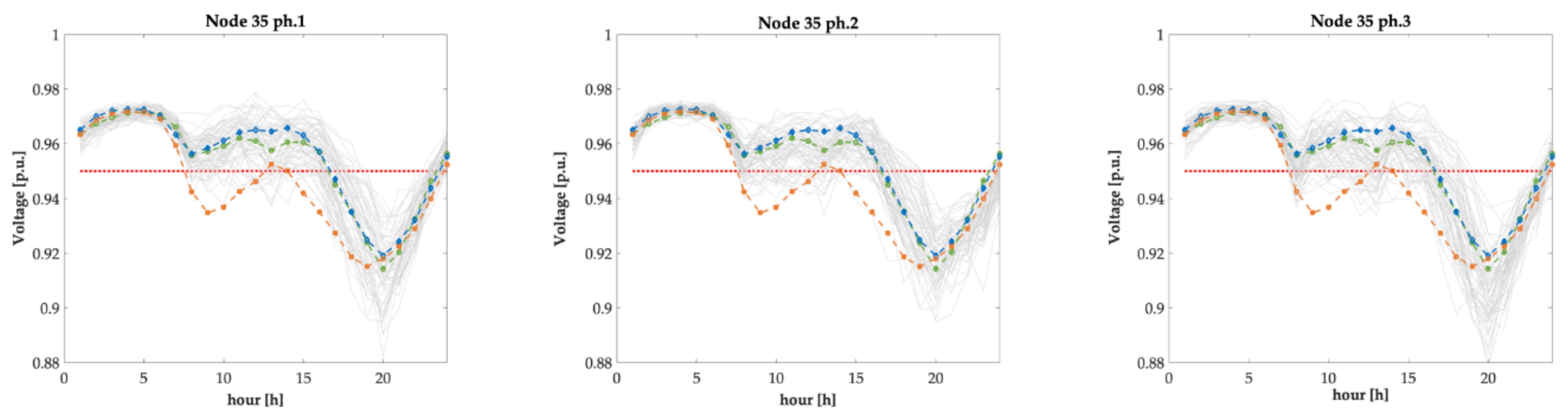Finally, as an example, Figure 21 shows the daily voltage profile of the node N_35 of Figure 17 which is at the farthest (i.e., about 400 m) from the sending end (i.e., the LV busbar of the MV/LV transformer). It is evident that the new typical load profiles better approximate the real behavior than the ones used by the DSO.

6. Conclusions

This paper proposes a methodology for finding typical load profiles for LV customers by using clustering techniques. Such a task is particularly challenging due to the great diversity of electricity use by such customers. The main scientific contribution of the paper is that new and updated LPs closer to the actual characteristics of customers of different categories are provided to the DSO, on the basis of recent and large databases gathered from extensive measurement campaigns, which covered much of the Italian territory. For reaching this goal, different clustering algorithms are exploited in a novel output-based approach that does not a priori prefer a specific clustering technique but uses one that provides the best results.

The results obtained by applying the proposed approach to several categories of end-users confirm the improvement in the accuracy of the network representation. The results demonstrate that one LP only for each category of customers is not enough to represent the actual behavior of LV customers, especially the residential ones that exhibit great variability in their consumptions. This result is convincing because the inaccuracy due to coincident peaks of groups of customers nominally homogeneous is overcome.

The comparison of two recent databases demonstrates that some characteristics of the customer electrical behavior were maintained over the period of a few years. Finally, this paper proposes an easy association of the most suitable typical load profile to new customers by considering only features available for the DSO (e.g., annual energy, rated power, monthly peak). Thus, it represents a concrete improvement of the state of the art and a step forward in the field of load profiling since the outcome of the research activity can be exploited in current real-life applications and the possible functionalities of advanced metering infrastructures are only partially enabled and would not fully be enabled in the near future. The proposed example of application of the LPs proves the validity of the approach.

Future works include the extensive application of the resulted profiles to operation and planning studies and the comparison of the typical load profiles of customers of different European Countries.