1. Introduction
In general, the value of the reliability index of a geotechnical structure, calculated using identical input parameters and assumptions, can vary significantly as a function of the applied method. The main reasons for this are related to assumptions and simplifications, which are introduced in the methods to simplify the reliability analysis. In other words, it is necessary to evaluate the reliability methods accuracies, i.e., research their suitability for application in different types of problem. Because of the differences in the mathematical expressions of the limit state definition among various geotechnical tasks, i.e., different forms of the performance function, it is not possible to give a generalized assessment of the suitability of a particular method of reliability to all geotechnical problems. However, it can be done on a case-by-case basis. The other possibility could be that a single method is suitable for application to a group of mathematically similar problems.
The main goal of this paper is to assess the suitability of common reliability methods in the case of the ultimate limit state (ULS) of shallow foundations. The suitability of the following methods was assessed: Analytical First Order Second Moment (FOSM) method, Taylor Series, Point Estimate Method (PEM), First Order Reliability (FORM) method, Simplified FORM, and the Monte Carlo method. For this purpose, the following sub-goals were set:
test the hypothesis of whether the factor of safety (FS) follows normal or lognormal distribution;
probability method error definition;
defining the criteria for method suitability assessment.
Analytical FOSM, Taylor Series and PEM reliability methods use FS as an objective function to calculate the reliability index, and their accuracy depends greatly on the assumed statistical distribution of FS. The paper analyses the statistic characteristics of the performance function, and shows that, contrary to a common assumption, the FS in the case of this study is not normally or lognormally distributed. In order to quantify the error which arises from the incorrect assumption of the FS statistical distribution, its actual probability density functions (PDF) were created using the Monte Carlo method. The results obtained were fitted with normal and lognormal PDFs, and error sizes were estimated based on the obtained results.
A review of relevant literature in the field of reliability in geotechnical engineering revealed a lack of information on the reliability method’s accuracy and the statistical distribution of the performance function in the case of the ultimate limit state (ULS) of a shallow foundation. Generally, a criterion to estimate the suitability of one or another reliability method for application in geotechnical engineering tasks was not defined. This paper defines such a criterion, based on the error size of the calculated reliability index (
). Using the proposed criterion, an assessment of the applicability of reliability methods was made, using a simple example of a centrally loaded foundation. The results obtained were compared to the results from other studies in the available literature: stability of the embankments from [
1] and retaining wall reliability [
2].
In general, Analytical FOSM, Taylor Series, PEM and FORM methods result in a reliability index, while the Monte Carlo and Direct Integration result in the probability of failure (
). In order to enable mutual comparisons in error sizes, the results of all methods were reported using a reliability index. The connection between
i
is defined by the following relation [
3]:
where
—the inverse Gaussian distribution
A detailed description of determining the reliability index using FOSM, PEM, FORM and the Monte Carlo is given in [
3]. What is generally emphasized, considering the accuracy aspect of each method, is that each method provides a different level of accuracy. Also stated is the problem of the statistical distribution of the performance function. In conclusion, it is reasonable and conservative to assume that it is distributed normally for safety margin (M), and lognormally for the factor of safety (FS).
Fenton and Griffiths [
4] conduct analyses of reliability in various geotechnical problems, using FORM, PEM, FOSM and the Monte Carlo methods. In the FOSM and PEM analyses, lognormally distributed performance functions are used. Using the example of ULS and the serviceability limit state (SLS) of piles subjected to a vertical load, they tested hypotheses that the performance functions are lognormally distributed. The soil’s influence on the pile was represented by bilinear springs, and the hypothesis was tested for different values of the coefficients of variations of spring stiffnesses (
). The hypothesis was confirmed for the ULS and the SLS, in the case where
. For greater
values—0.4 for ULS and 0.5 for SLS—the hypothesis was rejected. They conclude that a possible reason for the rejection in the sensitivity of the goodness-of-fit tests to small discrepancies in the fit, particularly in the tails, and that a lognormal distribution is a reasonable assumption.
Filz and Navin [
1] conduct reliability analyses using the stability of column-supported embankments (Case 1) and stability of embankments supported on panels under the side slope (Case 2). In their analyses, they use the Taylor Series method, PEM, Simplified FORM and the Direct Integration method. In the Taylor Series and PEM methods they choose the factor of safety (FS) for the performance function, and conduct analyses for the assumption that it is normally (Taylor Series and PEM) and lognormally (Taylor Series) distributed. The results of the conducted analyses are presented in
Table 1. They choose the Direct Integration as the control method, and use it to estimate the accuracy of other methods. As expected the Taylor Series and PEM give a significantly greater error when compared to Simplified FORM. A probable cause for such an error is an incorrect estimate of the statistical distribution of FS, as well as a simplification of the aforementioned methods. Considering the error size, they recommend using the Simplified FORM method exclusively to estimate the reliability in the examined cases. Although the most precise, they do not recommend the Direct Integration method due to its complexity.
Wang and Kulhawy [
5] analyse the relation of the reliability index for ULS and SLS of augered cast-in-place piles. They estimate the reliability indexes using FOSM, with the assumption of a lognormally distributed performance function. Due to the fact that the performance function can only assume positive values, and for mathematical convenience, such an assumption is considered reasonable.
Duncan [
6] promotes the usage of reliability methods in everyday engineering practices. He presents a procedure for determining the reliability index using the Taylor Series method. For the reliability index calculation, using the retaining wall and the slope stability examples, he assumes a lognormal distribution of the performance function, without assessing the reasonability of such an assumption. He claims there is no proof that the FS is lognormally distributed, but he believes that it is a reasonable approximation.
The accuracy of the Simplified FORM, PEM and Taylor Series methods in the example of sliding and baring capacity (undrained) of retaining wall is assessed by Duncan and Sleep [
2]. The results obtained were compared with the results of the Monte Carlo method, which is considered the most accurate of all methods used. PEM analyses were conducted for normal and lognormal distribution of the performance function, and the Taylor Series was used for the normal distribution. The arguments for the choice of the assumptions were not elaborated, and the results are presented in
Table 2.
Table 2 shows a good agreement between the Monte Carlo method results and the results of other methods. It is assumed that the good agreement is the consequence of the mathematically simple performance functions in the case studied.
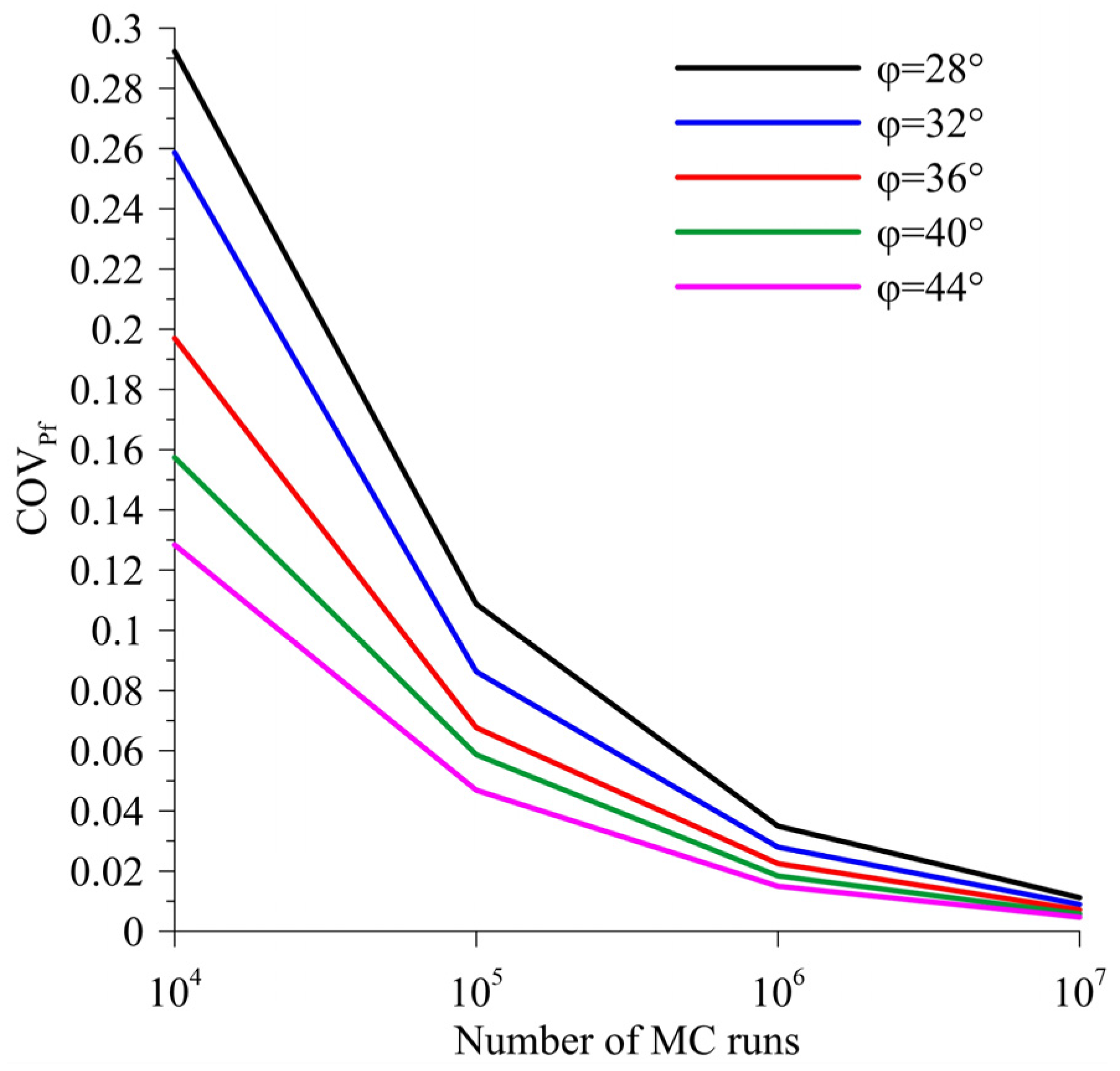
Considering the Monte Carlo method, Phoon [
7] claims that it is necessary to conduct
simulations for the coefficient of variation of
(
) to be less than 0.3. This paper confirms the stated hypothesis, and presents a graphic representation of the relation between the number of simulations and
.
The statistic characteristics of the performance function in the case of the SLS of the foundation are examined by Zhang and Ng [
8]. They analyse 375 bridge and 300 building settlement examples (SLS). They conclude that the performance function of the SLS of the structures follows a lognormal distribution. This information, along with the information on the distribution of the performance function in the case of ULS of the foundation, can be used for a more comprehensive estimate of foundation reliability.
Except in direct reliability calculations, reliability methods are used as parts of more complex procedures, e.g., in reliability-based optimization (RBO). To simplify the calculation work in RBO, Zhang et al. [
9] suggest replacing FORM with the simpler FOSM method. FOSM gives acceptably accurate results in linear performance functions and multivariant normal distribution. In other cases, the error can be large, but they believe that this can be rectified by finding the functional relationship between reliability indexes obtained using FORM (
) and FOSM (
), which they prove to be highly correlated.
Reliability Theory
Reliability as it is used in the reliability theory is the probability of an event occurring or the probability of a positive outcome. Evaluating reliability affords a means of assessing the degree of uncertainty involved in geotechnical engineering calculations [
2]. The complexity of reliability analysis, and consequently the reduced scope of its application, arises from the mathematical definition of reliability. It is defined as the complement of the probability of failure, which can be written as follows [
10]:
where:
—is reliability
—is the probability of failure
The probability of failure as a probabilistic event is mathematically defined by the following equation:
where:
—is a random vector
—is the performance function
—is the safety margin
Equation (3) could be rewritten using the reliability integral as follows:
where:
—joint probability density function of X
Considering the aforementioned, from a mathematical point of view it can be concluded that the basic task of reliability analysis is to calculate a multidimensional integral with joint PDF of random variables as integrand, and the integration domain defined by the performance function. The reliability problem containing the joint PDF
of 2 random variables (X1 and X2), and performance function
is visualized in
Figure 1.
The performance function cuts the joint PDF into two parts. The total volume under the surface equals 1. The smaller volume represents the probability of failure (
), and the larger, its complement, the reliability (
). The complexity of solving Equation (4) depends on the integrand, the performance function, and the number of variables. Depending on the degree of complexity and the availability of input data, a reliability integral can be calculated by direct integration of a multidimensional integral, or by using analytical or simulation methods [
11].
2. Materials and Methods
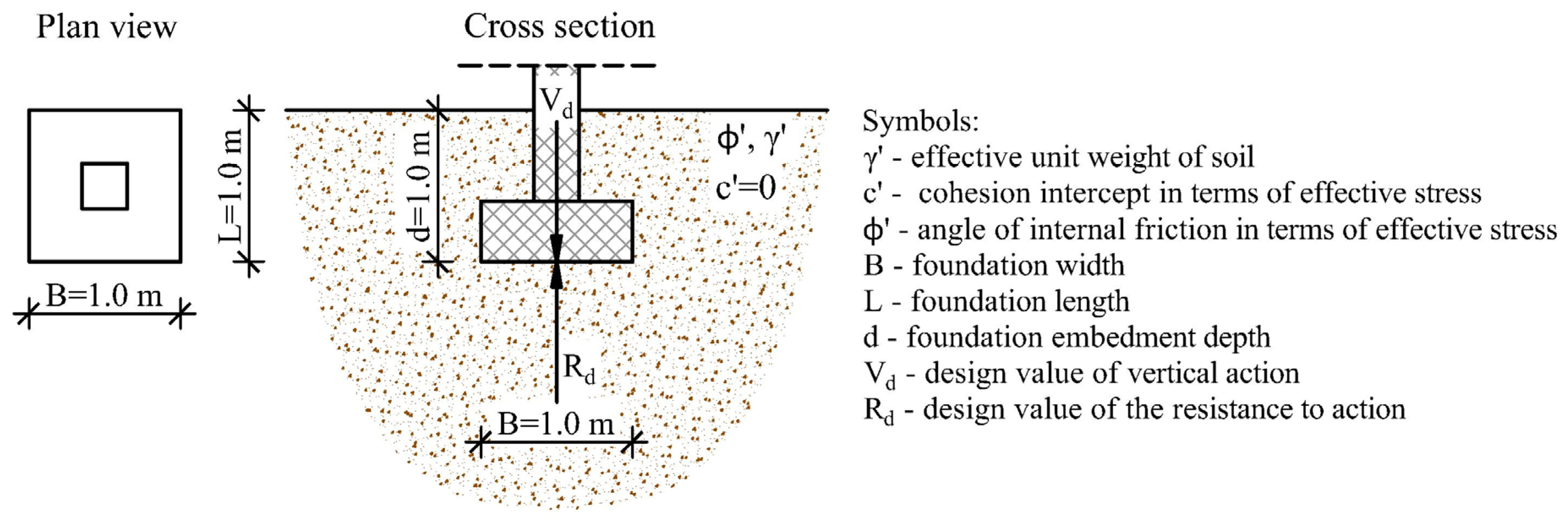
Reliability methods suitability assessments were performed for the ULS (bearing capacity resistance) of a 1.0 × 1.0 m centrally loaded square footing embedded in a non-cohesive soil at a depth of 1.0 m. The footing is subjected to a permanent vertical load. The model geometry is shown in
Figure 2. In a shallow foundation bearing capacity analysis, compared to the other parameters included in the analysis, the angle of internal friction is the dominant parameter that influences the outcome. Thus, a method suitability assessments were performed based on the results of parametric reliability analyses with variations of its value. All analyses were performed according to Eurocode 7 (EC7) [
12], design approach 3 (DA3), such that the design value of the vertical action equals to the design value of the resistance (
).
The value of
is calculated using the following equation [
12]:
where:
—is the permanent vertical force
—is the partial factor for permanent action, according to EC7, DA3
In reliability analyses, the following assumptions were introduced:
and
are random variables that follow normal distribution [
13,
14]
and are positive correlated, is uncorrelated with and
foundation soil is non-cohesive, homogeneous and isotropic
no presence of groundwater in the soil
Since the statistical scatter of geometric parameters is negligible compared to the scatter of geotechnical parameters and actions [
15,
16], they are introduced into the calculation as deterministic variables. According to [
13,
14], the
and
, and according to [
17],
can be considered as random variables with normal PDF. Statistical characteristics of random variables are shown in
Table 3, and their mean values used in parametric reliability analyses in
Table 4. The values of the coefficients of variation for random variables (
) were chosen from literature. Phoon and Kulhawy [
18] analyse variability in soil parameters, and they conclude that for soils with internal friction angles between 20° and 40°,
is within the range of 0.05–0.15. A slightly wider
range, 0.05–0.2, is presented by Phoon [
19], with the value depending on how the parameter is determined. Lee et al. recommend the use of
= 0.1 [
20] and the same value is used by Sujith et al. [
21] in reliability analyses of cantilever reinforced concrete (RC) retaining walls.
The typical value range for the coefficient of variation of soil unit weight (
) is 0.03–0.07 [
6]. Regarding the permanent load variability, various authors [
9,
22,
23,
24] use the value
in reliability analyses, therefore the same value was chosen for the analyses at issue.
In the parametric reliability analysis, the varied value is
, and the
values are calculated from the correlative relation of
and
according to [
25]. The
values is determined from the condition that
.
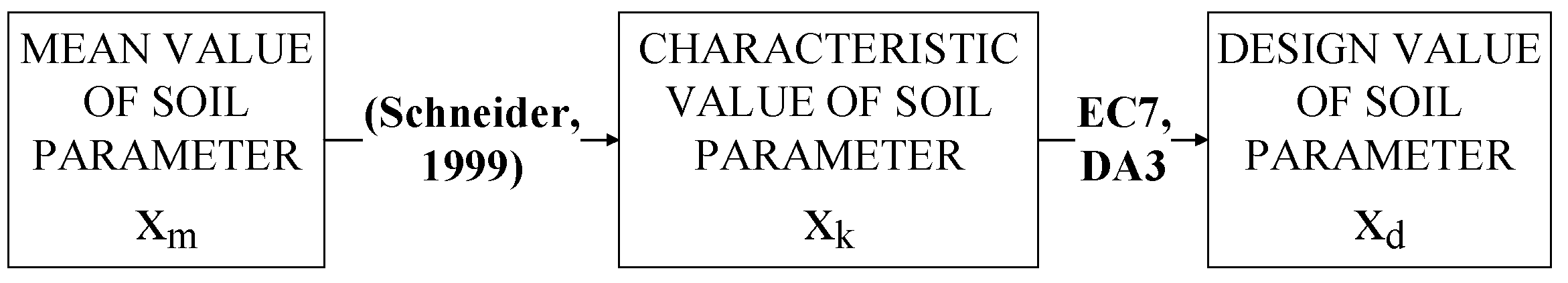
In calculations carried out according to Eurocode 7, the values of geotechnical parameters and actions will be characteristic or design. The characteristic values of
and
can be determined using statistical methods, based on available test results. Characteristic values are calculated from
and
according to [
26]:
where:
—is the mean value of X
—is the coefficient of variation of X
From the characteristic values, the design values are calculated in accordance with EC7, DA3. The flow chart for determining the values of geotechnical parameters is shown in
Figure 3. It is assumed that the characteristic value of permanent action corresponds to the mean value due to its low variability [
17,
24,
27,
28].
2.1. Performance Function
In general, the performance function in the structural reliability analysis is defined as follows [
10]:
—is resistance function, represents set of resistance variables
—is resistance function, represents set of load variables
In the case of a shallow foundation, R and S can be expressed as follows [
12]:
where:
—are bearing capacity factors
—are the base inclination factors
—are the shape factors
—are the inclination factors
—is the design effective overburden pressure at the level of foundation base
—is the effective foundation width
Equations for the “N”, “b”, “s” and “i” coefficients used for performance function definition were taken from Eurocode 7 [
12]. By including Equations (8) and (9) in 7 the following expression for the performance function in X space yields:
To simplify the reliability analysis, random variables X
1, X
2 and X
3 are transformed from the space of real random variables (X space) to the standard normal space (U space) using the Rosenblatt transformation [
29]. By applying the transformation, the performance function in U space yields:
2.2. Reliabilty Integral
The integrand of the reliability integral is a joint probability density function (PDF) of random variables. According to the assumptions of the random variable’s statistical distribution, the joint PDF is multivariate normal PDF, defined in
space as follows:
By combining Equations (4) and (12), the reliability integral takes the following form:
2.3. Defining the Error of the Reliability Method
The error of the method is defined as the maximum of the absolute difference between
calculated using the control method and the one calculated using the method whose accuracy is being assessed:
where:
—is the reliability index calculated using the method whose accuracy is being assessed
—is the reliability index calculated using the control method
In Equation (14), the maximum refers to the greatest error from the results of the parametric reliability analyses. The Direct Integration method was chosen as the control method.
2.4. The Criterion for the Estimation of the Suitability of Reliability Methods
To define the criterion for the estimation of the suitability of reliability methods, the classification of a structure’s expected performance level according to the reliability index was used [
16]. Concerning the
value, 7 classes of structure expected performance levels are defined: from Hazardous for
, to High for
.
Based on the classification, the size of the acceptable reliability method error (
) is defined as half the width of the class in which the accurate value
is located. Accordingly, the following applies: for
,
, and for
,
. Meeting these criteria will ensure a 50% probability that the reliability index (including error) is within the calculated class of the expected performance level, along with the largest error in the classification for a 1 class (
Table 5).
2.5. Short Overview of Reliability Methods
Reliability analyses using the FOSM analytical, Taylor Series, FORM and Simplified FORM methods were conducted using algorithms developed in Matlab programing language, while the Monte Carlo simulations were conducted in an application developed in the c# programming language. All of the used algorithms are validated by the computer program “Rt” [
30]. Compared to “Rt”, the developed algorithms are adapted to the problem in question, simplified in data input, include the calculation of the design value of permanent vertical action according to Eurocode 7, and provide additional possibilities when printing out the results. The algorithm used for conducting the Monte Carlo simulations is optimized for quicker execution and additional printing possibilities, e.g., the graphic representation of the histogram of the performance function and the dependence of the
value to the number of simulations. Direct integration was performed using an algorithm developed in the
c# programming language and
.NET Core framework. Analyses done using the Analytical FOSM, Taylor Series and PEM methods were performed with the assumptions that the FS follows both normal and lognormal distribution. The following abbreviated notation was adopted for easier assumption recognition: normally distributed FS—method name N; lognormally distributed FS—method name LN.
2.5.1. Analytical First Order Second Moment (FOSM) and Taylor Series
Analytical FOSM and the Taylor Series methods belong to the FOSM method group. Only the first terms of a Taylor series expansion of the performance function are used. They are used to estimate the expected value (Equation (15)) and variance (Equation (16)) of the performance function (F). If the number of uncertain variables is N, this method requires evaluating N partial derivatives of the performance function [
3]. The expressions for expected value and variance are defined as follows:
With calculated mean and variance, the reliability index β can be determined as follows:
The function F could be any relevant function, but for the purposes of this paper it is the factor of safety. The second-moment estimation (Equation (16)) is simplified in Taylor Series methods. It is assumed that this simplification can result in a large error, especially in cases where the
is a mathematically complex function. To estimate the error of FOSM methods without simplification in the second-moment estimation, direct calculation evaluating the partial derivatives with respect to all random variable is performed. In the Taylor Series method, the second-moment is approximated using the following formula:
where:
—FS calculated with the value of i
th parameter increased/decreased by one standard deviation from its mean value [
6].
2.5.2. Point Estimate Method (PEM)
PEM is the procedure used for determining the lower order moments of the performance function, done by determining its value on a set of carefully chosen points. The method was first introduced by [
31], and the detailed PEM calculation procedure used in this paper is described in [
2]. The number of required calculations in a single reliability analysis is 2
N, where N is the number of random variables. In these calculations, the value of the factor of safety is calculated with different combinations of random variables values, which are
and
(E(X) is the expected value, and
is the standard deviation of random variable X). The result is the reliability index
, which is calculated based on the assumption of statistical distribution of the FS.
2.5.3. First Order Reliability Method (FORM)
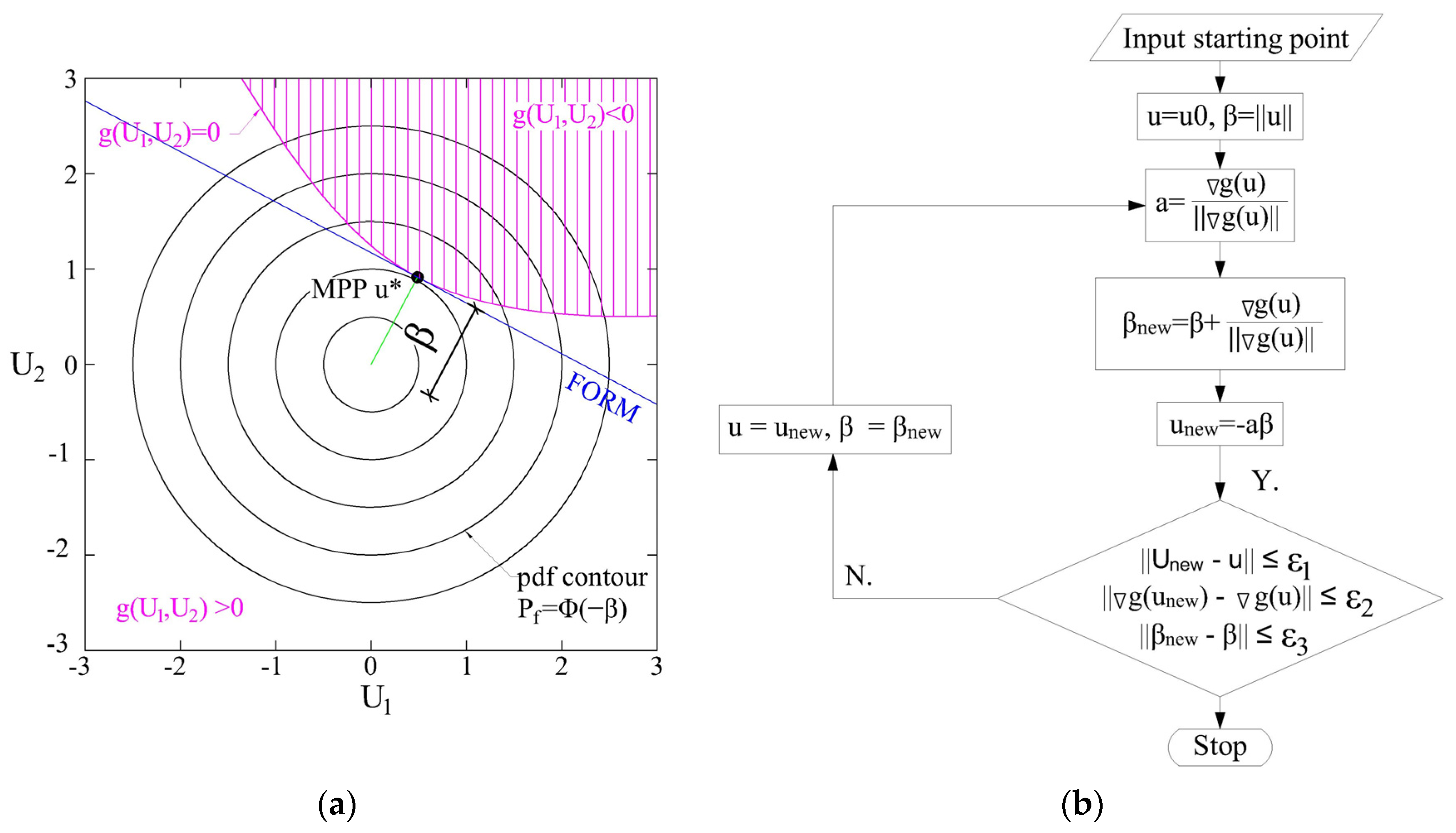
Unlike the FOSM methods, the FORM method includes information on the probability density function (PDF) of all random variables, and the limit state function is expanded at the point on failure surface, instead of the point where all variables have a mean value. The method represents an iterative procedure of searching for the point with the greatest probability density which is located on the failure surface. This point is called the most probable point (MPP), and it is used for the approximation of the performance functions [
30]. Random variables need to be transformed into uncorrelated standard normal variables, while the limit state function is transformed into standard normal space. The reliability index is then defined as the shortest distance from the origin to the failure surface (
) in standard normal space (
Figure 4a).
An iterative procedure (Newton–Rapson algorithm), shown in
Figure 4b, was used to calculate the reliability index. The iterative procedure was repeated until all three conditions were met in terms of error size:
(
Figure 4b).
2.5.4. Simplified FORM
The calculation procedure, according to the Simplified FORM method used in this paper, is described in detail in [
2]. It consists of three main parts. The first part is an iterative procedure in which the value of the reliability index is assumed, to calculate the reduced values of parameters. The factor of safety is then calculated using the reduced values. The procedure is repeated until the value
for which FS = 1 is found. In the second step, the change of FS for a given change in each set of random variables is determined. Each variable value from the set of values obtained in the final iteration of the first step is increased or decreased by 10%. The variable values related to capacity are increased, while the ones related to demand are reduced [
1]. The gradients obtained are then used to calculate the coefficient
which is the base for modifying the variable values used in step 3. The final, third step is an iterative procedure similar to the first step, with the intention of finding
for which FS = 1 applies. The difference from the first step is that the input parameter values were calculated using the
value calculated in the previous step. The resulting
represents the reliability index. Iterative procedures from steps one and three stop when the following criteria are satisfied:
.
2.5.5. The Monte Carlo Method
Monte Carlo simulation (MCS) is a numerical process of repeatedly calculating a mathematical or empirical operator in which the variables within the operator are sampled according to the prescribed probability distributions [
33]. The expected p
f values in the researched examples are in the order of magnitude
; therefore, a relatively large number of simulations is required to achieve satisfactory result accuracy. The coefficient of variation is calculated according to the procedure defined in [
34]. Random values were generated using the Mersenne Twister 19,937 algorithm from the open (MIT/x11 License) library of MathNet [
35].
2.5.6. Direct Integration Method
The reliability integral (Equation (13)) is approximated by the Riemann sum [
36]. Integration boundaries for each variable in the standard normal space were defined on a closed interval [−6, 6], with the number of discretization levels m = 3000. Considering the form of the integrand, integration boundaries are determined empirically so that the points in their vicinity make a negligible contribution to the result, also taking into account the recommendation given by Gong et al. [
37]. They recommend defining the limits of integration in standard normal space within the [−5, 5] range, since this ensures a probability lesser than
for uncertain input parameters to fall outside this range, which they consider to be negligible. The number of numerical integration points for a system with 3 random variables is approximately
. The detailed integration procedure is described in [
37]. Due to such a large number of integration points and mathematical complexity of the reliability integral, the integration was carried out on the computational cluster “Isabella”. The cluster was founded in 1971 within the University of Zagreb Computing Centre (SRCE) and it is intended for high-performance computing (HPC) for research projects and education. The individual integration job was divided into segments. Each segment of the calculation was performed on a separate processor in parallel, which significantly accelerated execution time. To verify the direct integration algorithm, its results were compared to the results of the Monte Carlo method with a relatively large number of simulations (
). The difference in the results between the two methods was in the 5th decimal place. Due to such a high degree of agreement of the results, it is considered that the direct integration algorithm is sufficiently accurate to assess the error of the other methods.
4. Discussion
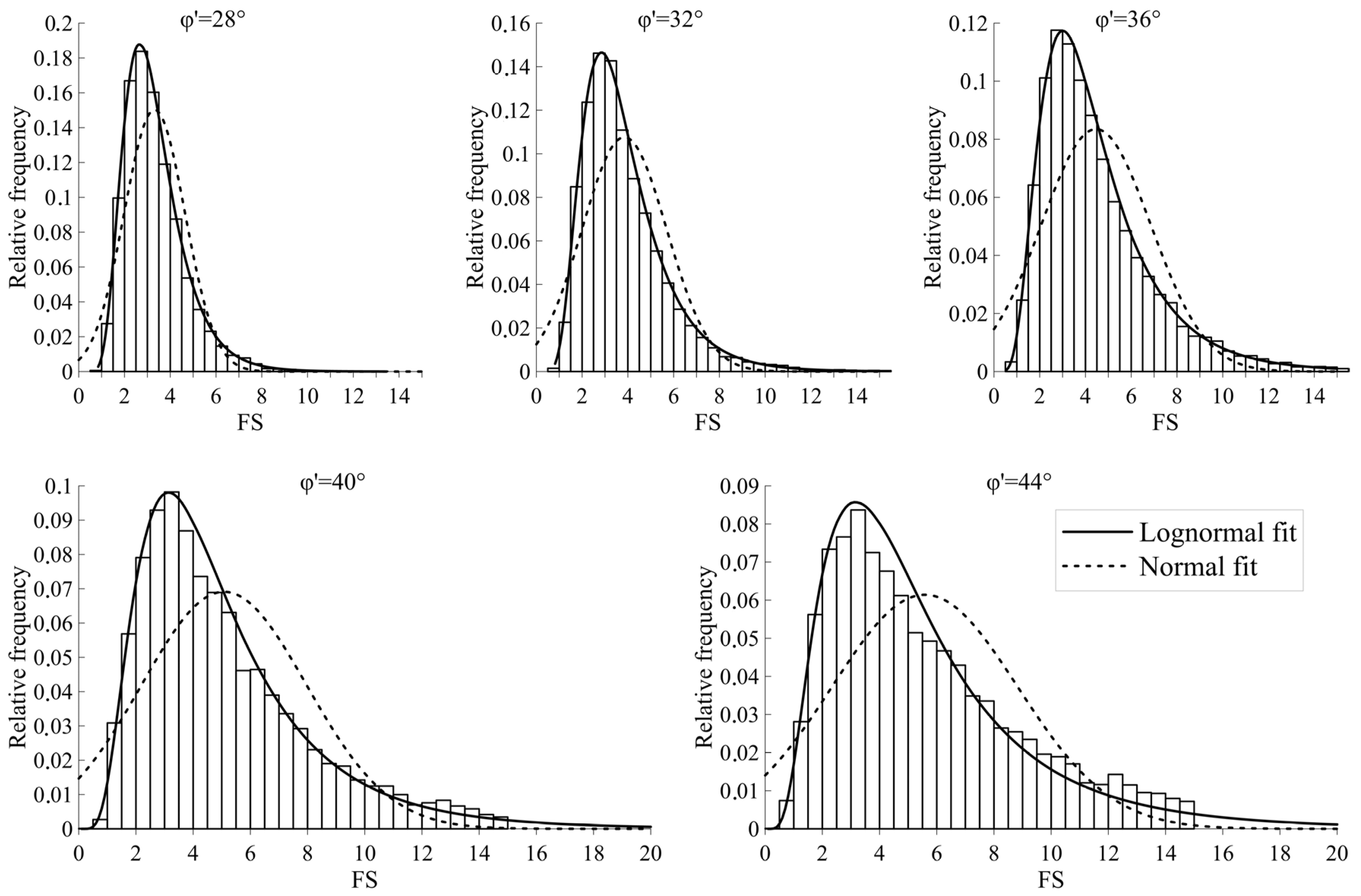
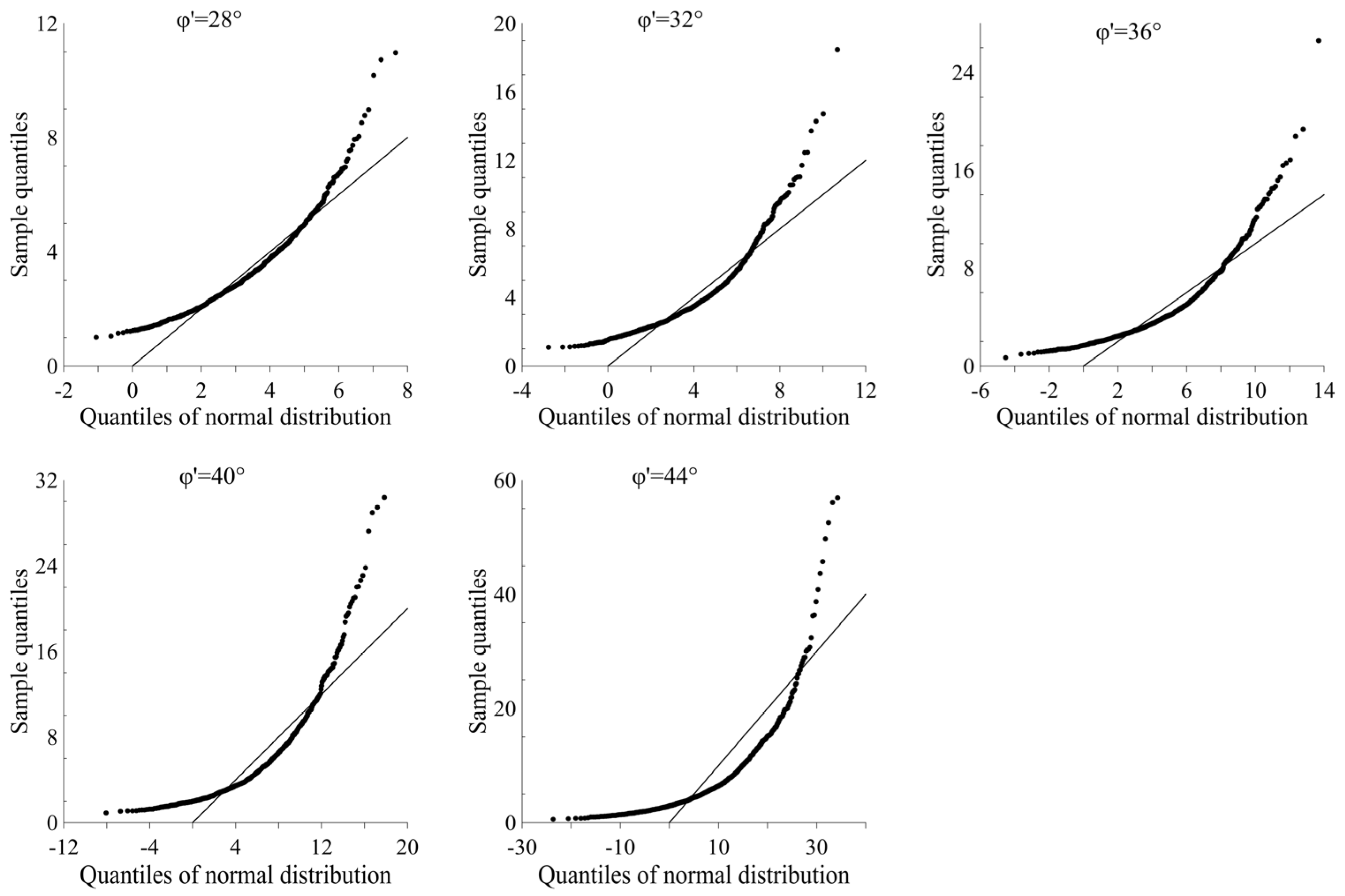
The paper shows that the FS for the ULS of shallow foundation is neither lognormally nor normally distributed (
Figure 5,
Figure 6 and
Figure 7), i.e., its actual PDF is unknown. Nevertheless, due to the similarity of the lognormal PDF and the actual PDF of FS, the claim from [
1,
2,
3,
4,
5,
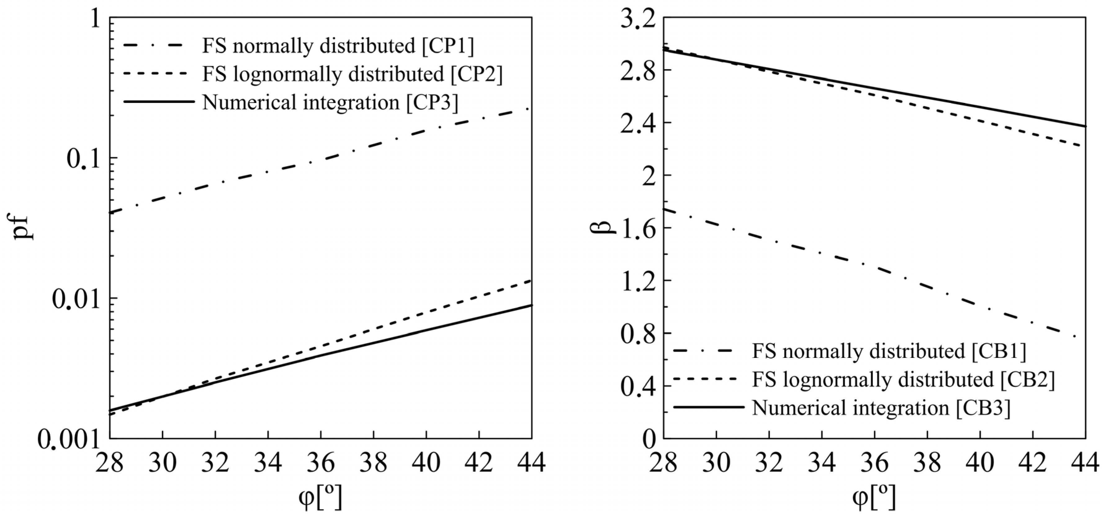
6] according to which it is reasonable to assume a lognormal distribution of FS may be acceptable for use in everyday engineering practice, under certain conditions—e.g., when used in combination with the Monte Carlo method or Analytical FOSM method (
Figure 8 and
Figure 9).
The reason for this is a relatively good match between the actual PDF of FS and the PDF of lognormal distribution. For different internal friction angles, good matching of the two PDF curves ranges up to the 98th percentile for
, and the 93rd percentile for
(
Figure 7). These findings are in agreement with the results of the study which analysed the statistic characteristics of the performance functions in the case of ULS and SLS piles [
4]. Much like this study, most of the theoretical curve and the actual PDF of FS match well, with larger deviations visible only in their tails. In the case of normally distributed FS, which was used for reliability analyses [
1,
2,
6], the error size is significantly larger. Such a result is expected, since the deviations between the actual PDF of FS and the fitted normal PDF are large (
Figure 5 and
Figure 6). This leads to a conclusion that the dominant cause for error in the Taylor Series and PEM methods arises from the simplification in the mean values and variances of the performance function estimations (
Figure 8), and not from an incorrect approximation of the distribution of the performance function. The claim from [
3], according to which a lognormal approximation leads to a conservative estimate of the reliability index, partially matches the results of this study, but only with friction angles larger than
. Contrary to this, in all analysed cases a normally distributed FS leads to a conservative approximation of
(
Figure 8).
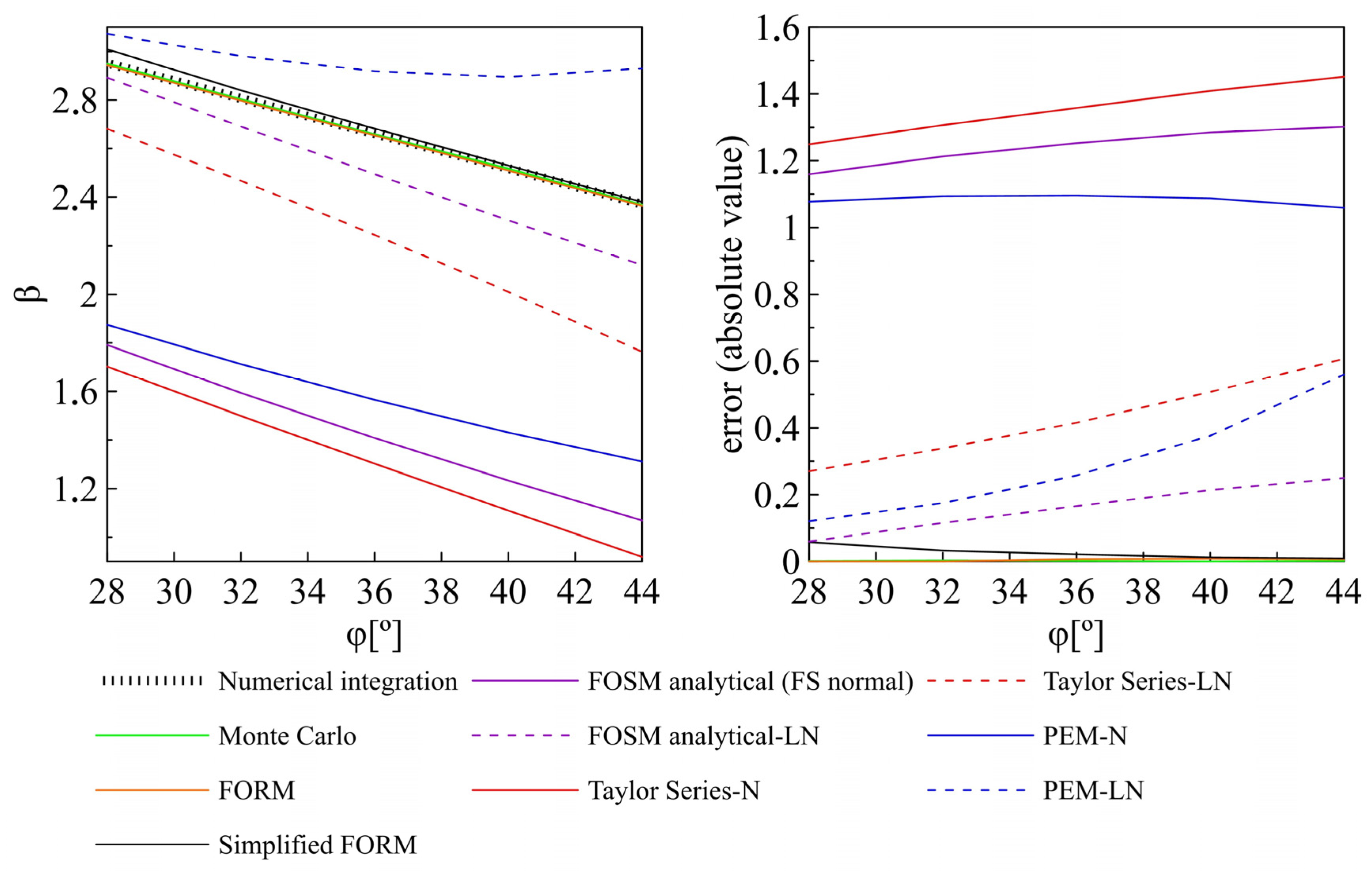
Figure 9 clearly shows a positive correlation between the reliability index calculated using the methods from the FOSM group and FORM, which matches the data from the study using this correlation for the modification of the RBO procedure by replacing the FOSM method for FORM [
9].
The results of the reliability methods suitability assessments in the case of the ULS of shallow foundation are shown in
Table 8. The Monte Carlo method, FORM and Simplified FORM methods result in a negligible error up to 0.05 and FOSM analytical-LN in a slightly greater error—up to 0.25 (
Figure 10). According to the proposed criterion (
Section 2.4), they are suitable for a reliability assessment of the footing researched in this paper. Introducing additional variables, e.g., load eccentricity or soil cohesion, might result in larger errors; with the exception of the Monte Carlo method, their suitability should be checked for shallow foundation reliability analysis in general.
The Taylor series, PEM and FOSM analytical with normally distributed FS result in a large error, ranging from 0.56 to 1.45. Based on the reliability method suitability assessment, it is concluded that they are not suitable for reliability assessment of the shallow footing researched in this paper. Since the problem researched in the paper is fundamental in the sense of applied load and soil type, the conclusion regarding the Taylor Series, PEM and Analytical FOSM-N can be extended to the reliability analysis of footings in general, also taking into account more complex types of actions and ground layering
For example, a reliability analysis of a footing embedded in coherent soil, loaded with different types of action, will include more random variables, and consequently a mathematically more complex reliability integral formulation. This will affect the shape of the actual PDF of FS and additionally contribute to the uncertainties in the first and second moments estimation.
The results of the reliability method suitability assessment of the ULS of shallow foundation are in agreement with the results of the study dealing with embankment stability [
1]. This study concluded that the Taylor Series and PEM methods are not appropriate for the estimation of the reliability of embankment stability and recommends using only the Simplified FORM method (
Table 1). It is presumed that such a conclusion was reached based on the error sizes for the methods considered. The criterion defined in
Section 2.4 was applied to the data from this study, and the results are shown in
Table 9. The results obtained perfectly match the conclusions of the study authors, even though they did not explicitly list the criteria which led to their conclusion.
The same criterion was applied to the data from the study (
Table 2) which researched retaining wall reliability for three failure modes: sliding on sand, sliding in clay and bearing capacity (undrained) [
2]. Unlike the previous two examples (shallow foundation and embankment stability), the performance functions are significantly simpler, which generally yielded smaller errors for all the methods used (
Table 10 and
Table 11). The Simplified FORM method is suitable for the reliability assessment of all three failure modes, while PEM-N is not suitable for either. The Taylor Series-N method is suitable for reliability analyses of sliding on clay and bearing capacity, while the PEM-LN method is suitable for reliability analyses of sliding on sand and sliding in clay.
Based on the results presented, a conclusion is reached on which methods are suitable for use in the presented geotechnical engineering tasks. In general, simpler methods are not recommended in everyday engineering practice without previous validation in the task at hand. Doing otherwise can lead to incorrect reliability measurements, which will be impossible to identify as an under- or overconservative solution. This is also applicable for more complex reliability analyses, such as the RBO, since these procedures use previously listed methods.
Although not the subject of this paper, the reliability analyses showed significant differences in reliability indexes (ranging from 2.38 to 2.94) of the footing for different angles of internal friction. All analyses were performed for the ULS according to Eurocode 7, DA3, for the case when
. The target
value for the reference period of 50 years is 3.8 [
17]. Calculated reliability indexes are significantly lower than the recommended value; therefore, a question of design procedures evaluation according to EC7 can be raised. The recommendation for further research is to analyse the reliability indexes of different types of geotechnical structure designed according to Eurocode 7 and the possible introduction of additional partial factors of safety elaboration regarding the degree of understanding of the site-specific conditions. A similar principle is prescribed in the Canadian Highway Bridge Design Code [
38], which allows engineers to have their designs reflect the degree of uncertainties associated with the parameters and models used [
39].


