Hybrid Machine Learning Model for Body Fat Percentage Prediction Based on Support Vector Regression and Emotional Artificial Neural Networks

Abstract

Obesity or excessive body fat causes multiple health problems and diseases. However, obesity treatment and control need an accurate determination of body fat percentage (BFP). The existing methods for BFP estimation require several procedures, which reduces their cost-effectivity and generalization. Therefore, developing cost-effective models for BFP estimation is vital for obesity treatment. Machine learning models, particularly hybrid models, have a strong ability to analyze challenging data and perform predictions by combining different characteristics of the models. This study proposed a hybrid machine learning model based on support vector regression and emotional artificial neural networks (SVR-EANNs) for accurate recent BFP prediction using a primary BFP dataset. SVR was applied as a consistent attribute selection model on seven properties and measurements, using the left-out sensitivity analysis, and the regression ability of the EANN was considered in the prediction phase. The proposed model was compared to seven benchmark machine learning models. The obtained results show that the proposed hybrid model (SVR-EANN) outperformed other machine learning models by achieving superior results in the three considered evaluation metrics. Furthermore, the proposed model suggested that abdominal circumference is a significant factor in BFP prediction, while age has a minor effect.

1. Introduction

Obesity is a public health problem worldwide [1]. Researchers predict that obesity causes several major health issues, such as mood disorders, cardiovascular diseases, respiratory ailments, and digestive issues [2]. In the medical, healthcare, and fitness sectors, a person is determined as obese by calculating the person’s body mass index (BMI), which considers the person’s body weight divided by body height square [3]. BMI is a beneficial measurement, particularly for population-based screening. However, subgroups of obese individuals with normal metabolic health but a higher body mass index or obese individuals with poor metabolic health but an average body mass index exist [4]. Therefore, BMI might not capture people at a higher risk of cardio-metabolic disorders, such as type 2 diabetes and cardiovascular disease.

The lack of effective information from BMI changed researchers’ focus to body fat percentage (BFP), which measures fat in the body and provides a more accurate assessment. However, to criticize the amount of obesity and prevent it, it is critical to precisely assess BFP. Several methods can accomplish the estimation of the BFP. Some approaches, such as anthropometry models, consider the age, weight, waist circumference, and skinfold thickness of a person to make assumptions based on physics laws and mathematical computations [5]. Other clinical approaches use special instruments to measure body composition. However, models such as underwater weighing (UWW), dual-energy X-ray absorptiometry (DEXA), bioelectrical impedance analysis (BIA), computed tomography (CT), magnetic resonance imaging (MRI), and near-infrared interactome (NIR) are more accurate and more expensive. Researchers who have studied the BIA instrument relied heavily on body composition measurement and estimation of BFP throughout the last few years [6]. However, the above-mentioned methods could produce ineffective estimation either in terms of cost or inaccuracy. Therefore, researchers have begun to use the capabilities of artificial intelligence (AI) and machine learning (ML) models to solve a complex non-linear problem as a cost-effective and more accurate alternative for BFP prediction. This led to the proposal of high-performance prediction models for BFP from simple anthropometric measurements and basic information such as gender and age using several machine learning models.

The most commonly and frequently used models for BFP prediction are artificial neural networks (ANNs) and support vector regression (SVR), which can create non-linear relations between the limited number of instances [7]. Kupusinac [1] employed an ANN to predict the BFP, and they considered the age, gender, and BMI of the persons as instances for the prediction of BFP in their study. In addition, Ferenci [8] explored how relevant features are in predicting BFP in the presence of 39 anthropometric and laboratory measurements using ANNs and SVR. It was concluded that waist circumference is the most associated trait with a successful prediction of BFP. However, the uninterpretable data processing and output prediction of ANNs prevented the determination of the importance and the impact of relative input features in BFP prediction, even though considerable prediction results were achieved.

Furthermore, Chiong et al. [9] presented an improved relative error support vector machine to predict BFP. Their study considered two datasets: a body fat dataset [10] and 39 anthropometric and laboratory measurements of 852 observations. The proposed model included a bias error control term, and their feature selection model was based on removing irrelevant features. Even though the proposed model had high prediction ability for BFP prediction and considered a large number of features, it still lacked interpretation of the significant features that affect BFP prediction.

All these studies showed the ability of machine learning models, particularly the ANN and SVR, to predict BFP using minimized data that do not require the utilization of some outer information-handling units. However, the variety of machine learning (ML) models and the proposal of different types of neural networks led to the implementation of different ensemble or hybrid models in order to increase the prediction ability for BFP.

Generally, hybrid machine learning approaches that utilized forecasting models that incorporated two modeling algorithms were offered [10]. The initial algorithm of hybrid models recognizes and determines the variables that play a significant role in explaining the model’s outcomes but whose number is limited. The following algorithms of the hybrid model use explanatory variables to create predictions. Therefore, improved prediction rates are achieved using the abilities of different algorithms.

Shao [11] and Ucar [12] constructed hybrid models based on a multilayer feed-forward neural network (MLFFNN), SVM, decision tree (DT), and linear regression (LR) to optimize feature selection models. These studies used a body fat dataset developed by Johnson [10], including 14 attributes of 252 males. It was concluded that an anthropometric measurement could effectively be considered for predicting BFP; however, the investigation of gender effect was ignored because of not including female data.

The employment of feature selection models to criticize significant features is crucial for the performance enhancement for BFP prediction. Therefore, studies [11,12] proposed hybrid models for feature selection and multiple ML prediction algorithms with high prediction rates. However, these models used relatively small datasets with a restricted number of male samples, and their proposed models were never tested with relatively large datasets.

The improvements of the ANN to advance the performance [13] or to consider human emotions to improve the learning abilities of neural networks were investigated in different studies [14,15], and recently, emotional artificial neural networks (EANNs) were proposed [16]. In EANNs, the “emotion” ties to the activity of neurophysiological reaction in biological terms: humans might be capable of changing their response to situations using their attitudes and emotions. Thus, an input circle is established by combining the neuronal and hormonal frameworks. This improves the model’s learning capacity, reduces computational costs, and provides effective convergence with limited data [16]. The robustness of the obtained results led the EANN to be implemented in various fields, such as forecasting the steady cross-sectional math of alluvial channel profiles [17], forecasting suspended silt loads [18], and the prediction of the strength of concrete under compression [19].

Based on the above-discussed information, ML-based BFP prediction requires hybrid studies with comprehensive and primary datasets and features besides the performance of the algorithm. In this study, we proposed a hybrid ML model (SVR-EANN) by combining support vector regression and emotional artificial neural networks. The model includes a feature selection procedure using SVR and uses the prediction ability of EANN, which combines the basic structure of the neural network with various emotional functions, to achieve high prediction rates and determine the most significant factors that affect BFP. In addition, a primary dataset, including age, gender, height, weight, abdominal circumference (abdominal C), waist-to-hip ratio (WHR), which implies the ratio between waist circumference and hip circumference, BMI, and BFP, was considered. The analysis and prediction of BFP using a higher amount of data in terms of instances, including both genders, and minimized number of attributes could provide more accurate prediction rates and help researchers determine significant factors affecting BFP. In addition, the investigation and development of new hybrid models to perform feature selection and prediction have crucial importance in improving prediction ability. Finally, the obtained results were compared to the eight benchmark ML algorithms, namely, feed-forward neural network (FFNN), EANN, SVR, DT, random forest (RF), linear regression (LR), gradient-boosting algorithm (GradBoost), and extreme-gradient-boosting algorithm (XGBoost), and recent research. Based on the above-mentioned information and obtained results, the contribution of this study could be listed as:

• Collection of primary data for BFP prediction with a higher number of observations for anthropometric attributes for both genders.
• Employment of the WHR for the first time in a machine learning prediction model for BFP.
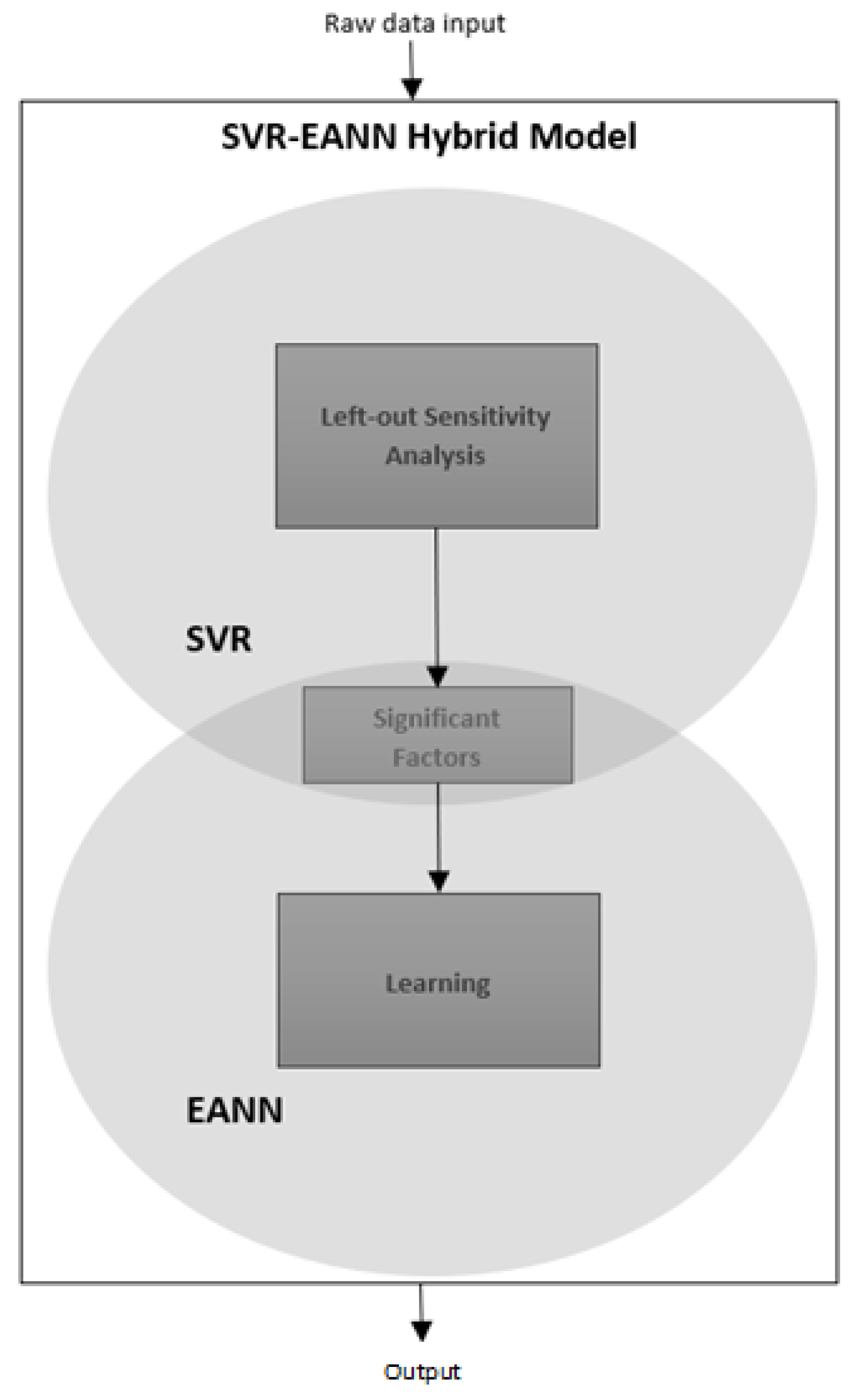
• Creating a hybrid model for accurate prediction of the BFP.
• Feature selection and the most influential factor determination using SVR and left-out sensitivity analysis.
• Prediction of BFP using the selected features and EANN.
• Comparison of the results with benchmark machine learning models.

The rest of the paper is organized as follows: Section 2 introduces the dataset, the machine learning models used in the hybrid model, and the evaluation strategies. Next, Section 3 explains the proposed hybrid model in detail. Then, Section 4 presents the experimental results and discussions. Finally, Section 5 concludes the remarks of the study.

2. Materials and Methods

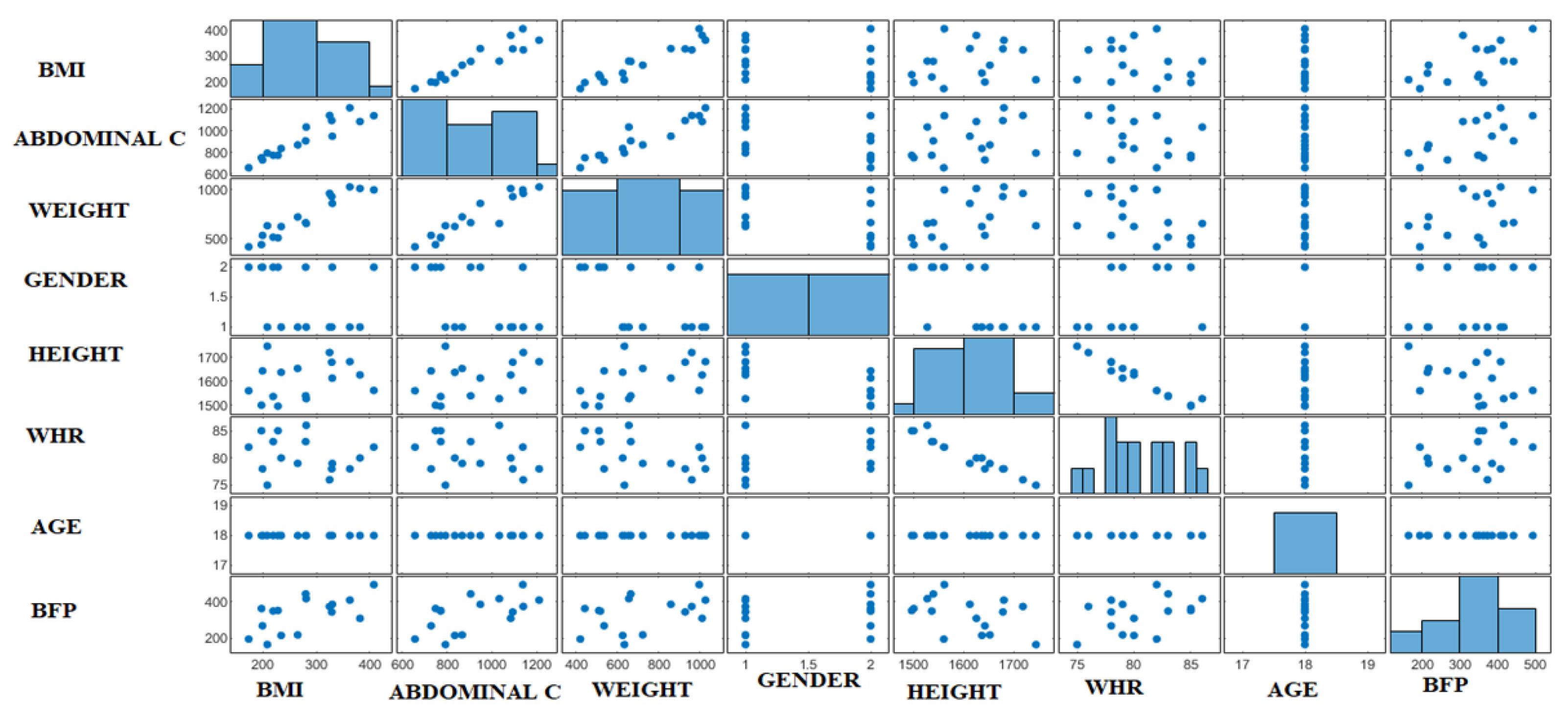
2.1. Datasets

The aim of collecting primary data for this study was to develop a BFP prediction model capable of predicting BFP with high accuracy rates using the relevant anthropometric attributes and determine the most significant parameters that affect the prediction model. The dataset consisted of eight attributes (gender, age, height, weight, abdominal C, WHR (the ratio of waist circumference/hip circumference), BMI (weight/height²), and BFP). The BFP was estimated by a body composition analysis device named BIA ACCUNIQ BC380 positioned in the Department of Food and Nutrition of Baxshin Hospital, Iraq, under the supervision of specialized doctors. The abdominal C in this study represented the waist circumference which is a “constant measure of abdominal obesity” [20]. Data were collected under the supervision of expert staff, and special procedures were followed to estimate the metric parameters as well as the body composition of 2000 observations of 387 males and 1613 females. The ages were between 18 and 29—the parameters were selected according to the importance of anthropometric models in historical research on BFP estimation.

The collected data consisted of a single observation for each person and did not contain time-series data to predict the future BFP by considering the person’s recent anthropometric and laboratory measurements. Therefore, the study focused on the accurate prediction of the recent BFP of a person to minimize the time and costs to obtain BFP. The summary of the descriptive statistics of the data is provided in

Table 1. Descriptive statistics of the dataset.

Parameters	BMI (kg/m2)	Abdominal C (cm)	Weight (kg)	Gender	Height (cm)	WHR (cm)	Age	BFP
Mean	26.218	86.6345	67.05	1.81	160.301	0.825	23.05	33.42
Standard Deviation	10.33	18.031	21.761	0.40	9.4638	0.0554	3.43	11.83
Minimum	12.9	60.7	15.40	1.00	63.00	0.66	18.00	3.00
Maximum	237.3	182.7	183.70	2.00	199.8	2.1	29.00	87.7

.

Initially, the Pearson correlation matrix was created to show the linear dependencies between the attributes (variables) and observe the strength of the correlation [21]. It was observed that BFP had a higher correlation with the BMI followed by the abdominal C and weight with correlation coefficients of 0.8086, 0.7583, and 0.6277, respectively. Age, WHR, and height were found to be the variables with the lowest correlation with the BFP. The correlation matrix between the variables and the graphical representation is shown in

Table 2. Coefficients of correlation matrix between the variables.

	BMI	Abdominal C	Weight	Gender	Height	WHR	Age	BFP
BMI	1
abdominal C	0.9531	1
weight	0.9279	0.9589	1
gender	0.0118	−0.155	−0.2183	1
height	−0.0036	0.1203	0.3288	−0.6017	1
WHR	0.0047	−0.0698	−0.2683	0.4822	−0.9358	1
age	0.2479	0.2042	0.2216	0.0289	−0.0059	0.0490	1
BFP	0.8086	0.7583	0.6277	0.4411	−0.3979	0.3643	0.2097	1

and Figure 1.

2.2. Machine Learning Models

This section presents the details of three models, ANN, EANN, and SVR, considered as base models for the hybrid model.

2.2.1. Artificial Neural Networks

Artificial neural networks (ANNs) aim to simulate and perform functional features similar to the biological neural network of the human brain. This provides the capability of learning relationships from examples, making them ideal for situations where there is no reliable relationship between input and output data [22]. ANN studies and applications differ and vary almost in every field of our lives and scientific fields such as economics [23] and neuroscience [24].

Even though several neural network types exist in the literature, the backpropagation (BP) neural network is the most widely and commonly considered ANN because of its efficiency and simplicity. Essentially, ANN consists of an input layer, at least one hidden layer, and an output layer where the number of neurons (nodes) in the input and output layer depends on the problem domain [25]. The determination of hidden layer numbers and the neuron numbers of the corresponding layers is a challenging task, and still, trial and error is the most effective way to determine the neuron numbers. The neurons are interconnected through the layers, and the summation function (net function) is used to obtain the general knowledge for each neuron and input. The activation function, commonly a sigmoid one, provides the outputs of most informative neurons depending on the information level, and generally, the gradient-descent algorithm is applied for error minimization during the convergence. The weights are adjusted accordingly and propagated back iteratively to achieve minimum error and to provide efficient convergence.

The equation of obtaining the output in ANN was described as shown in Equation (1) [26]:

$${\hat{\mathrm{y}}}_i=f_j\left({{\displaystyle \sum }}_{h-1}^m{w}_{jh} \times f_h\left({{\displaystyle \sum }}_{i=1}^n{w}_{hi}{x}_i+w_{hb}\right)+w_{jb} \right)$$

(1)

where i represents the input layer, h represents the hidden layer, and j represents the output layer. Weights and bias are denoted as W and b, respectively. X indicates the input value, and n and m stand for the number of input and output neurons, respectively.

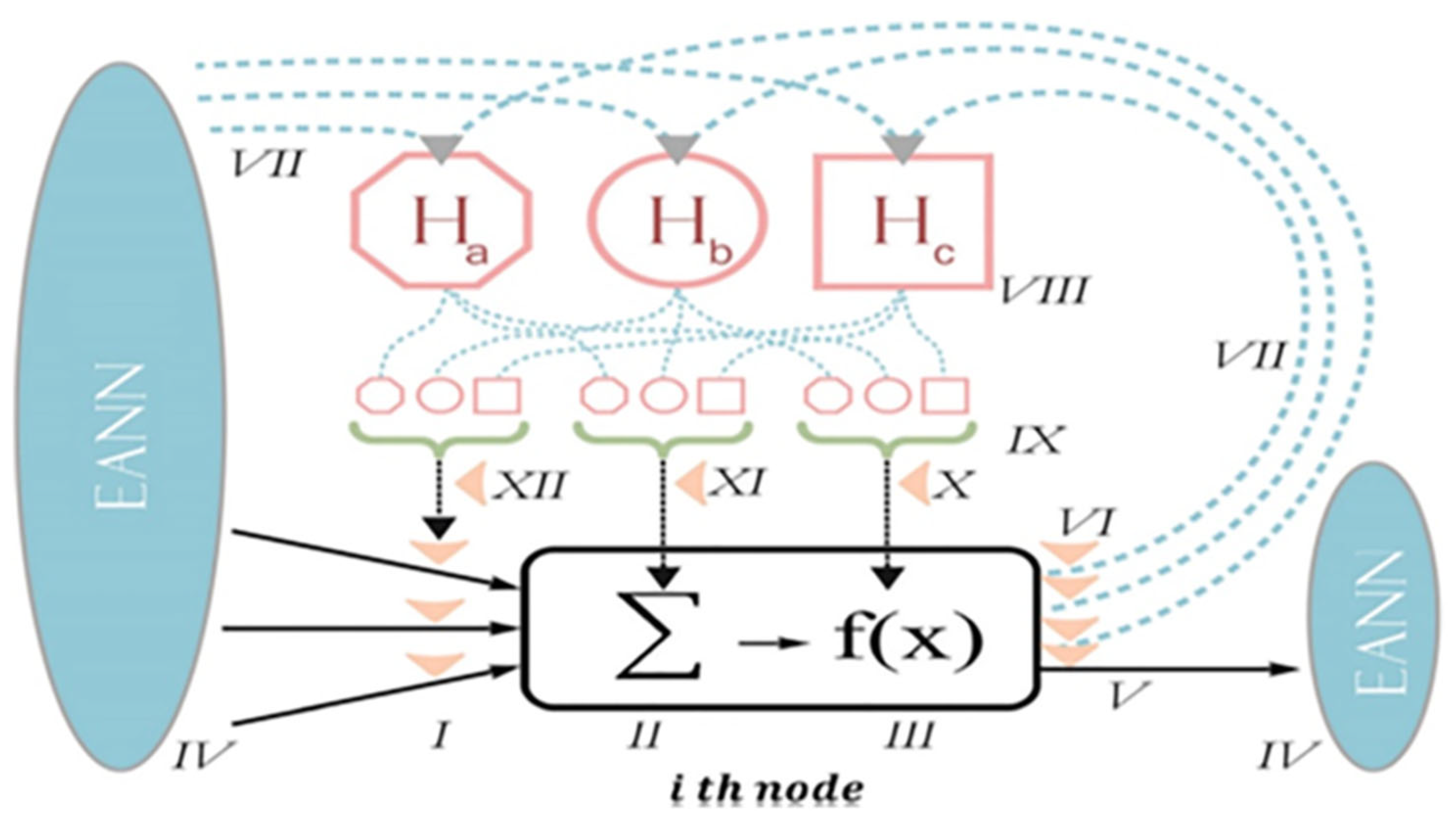
2.2.2. Emotional Artificial Neural Networks

The emotional system was included in the network structure of emotional artificial neural networks (EANNs), which is the improved version of ANN to allow neurons to generate hormones for altering cognitive, physical, and emotional capacities [16,27].

The EANN considers the hormones and hormonal weights to increase the convergence level of the network. Therefore, neurons’ input and output values are used to adjust three hormonal weights (H_a, H_b, and H_c) and the parameters of weight for activation function, summation function, input value, and bias value (∂, ζ, Φ, and χ). This procedure yields the reflow of all information through the layers and provides increased ability for the model. Figure 2 illustrates the general block diagram of EANN and demonstrates how each EANN neuron transmits information back and forth between the input and output nodes. Both neural and hormonal weights are considered for each iteration, and the weight adjustment operation is performed accordingly.

After numerous cycles, the model’s coefficients are attuned to patterns in the input and output and are then adjusted during the training process. Numerical coefficients of the hormonal factors influence the individual node elements, such as weight, activation, and summation function. The solid and dotted lines in Figure 3 represent the neural and hormonal lines. The output of i_th neuron of an EANN with three hormonal glands was described as shown in Equation (2) [16]:

$$Y_i=(\underset{1}{\underbrace{{\gamma }_i+{\displaystyle \sum }_h{\sigma }_{i,h}{H}_h)}} \times f[{\displaystyle \sum }_j(\underset{2}{\underbrace{({\beta }_i+{\displaystyle \sum }_h{\zeta }_{i,h} H_h)}} \times (\underset{3}{\underbrace{{\theta }_{i,j}+{\displaystyle \sum }_h{\mathsf{\Phi }}_{i,j,k} H_h)X_{i,j})}}+\underset{4}{\underbrace{({\alpha }_i+{\displaystyle \sum }_h{\chi }_{i,h} H_h)]}}$$

(2)

where i, h, and j represent the neurons of the input, hidden and output layers, f() is the activation function of the neuron. ∂, ζ, Φ, and χ are the parameters for activation function weight (Term 1 in Equation (2)), summation function (Term 2 in Equation (2)), input value (Term 3 in Equation (2)), and bias value (Term 4 in Equation (2)) that control the hormonal levels, respectively. The neural weights are represented as γ, β, θ, and α.

Then, the hormone value sum is calculated and imposed on the network as described in Equations (3) and (4), respectively.

$$H_h={{\displaystyle \sum }}_i{H}_{i,h}\left(h=a,b,c\right)$$

(3)

$$H_{i,h}=glandit{y}_{i,h} \times Y_i\left(4\right)$$

(4)

In which glandity was described as a calibration factor of providing suitable hormone levels during the training.

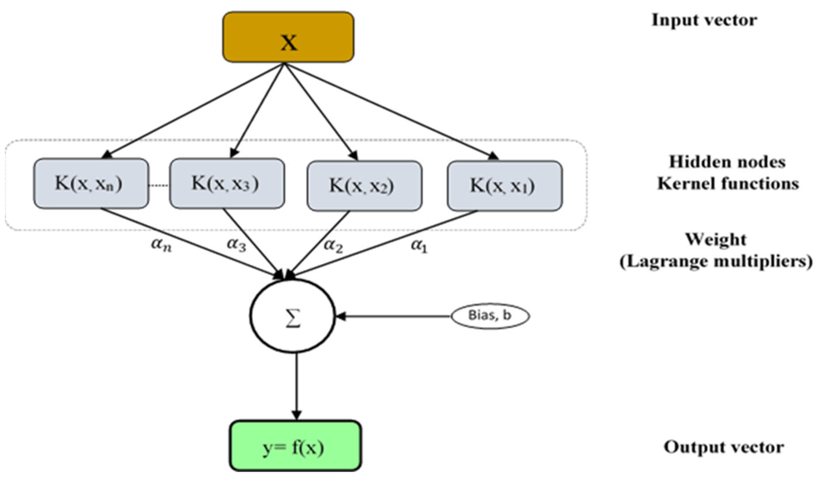
2.2.3. Support Vector Regression

Support vector machines were initially proposed for classification tasks [28] and implemented successfully in recent studies [29]; however, the model was modified to accept real-valued data and to be implemented for regression problems. The differentiation of support vector regression (SVR) from other machine learning models is the projection of data into another dimension using different kernels and considering the data points of projected kernels, not directly the data. This leads to choosing support vectors using data points for maximum efficiency and minimizes structural risk. The model’s efficacy for both linear and non-linear problems is obtained by mapping the data and converting non-linear data to linear separable objects in another hyperplane.

The general structure of the SVR model is shown in Figure 3, and the SVR equation is provided in Equation (5) [30]:

$$\left(x,{\alpha }_i,{\alpha }_i^{*}\right)={{\displaystyle \sum }}_{i=1}^N\left({\alpha }_i-{\alpha }_i^{*}\right)K\left(x,x_i\right)+b$$

(5)

where x and b represent the input vector and bias term, respectively, and Lagrange multipliers and the kernel function are indicated as α_i, ${\alpha }_i^{*}$, and K, respectively.

Considering projected support vectors using the kernel function K(x,x_i), which are the closest data points, results in minimized errors on the regression line. During this error minimization and function optimization, the Lagrange multipliers are used to find the local maxima and minima and provide the optimization. In this study, we used radial basis function (RBF) kernel, which is the most used kernel in the SVR [7,31].

2.3. Data Preparation, Validation, and Performance Evaluation

Since the dataset did not contain missing values, only a data normalization procedure was applied in the data preparation phase. Even though the normalization of data into a certain range is not an obligatory process for regression tasks, the normalization of the data has a significant effect on the performance of neural networks in terms of computational cost and prediction accuracy [31]. We normalized the data using Min–Max normalization, for which the formula is provided in Equation (6).

$$x_{norm}=\frac{x-x_{min}}{x_{max}-x_{min}}$$

(6)

where x, x_norm, x_max, and x_min are the input, normalized, maximum, and minimum observed values (instances) of the corresponding data attribute, respectively.

The main purpose of using machine learning models for regression problems is to achieve reliable results, which are difficult to obtain using traditional methods without prior knowledge and a deep understanding of the concept. However, due to overfitting problems in many ML models, the model’s performance at the training stage is not always coherent with its performance at the test stage, making it impossible to obtain accurate prediction results for other unseen datasets. This makes it vital to validate the models to overcome the overfitting issues.

Different types of validation processes exist in the literature (k-fold cross-validation, holdout validation, leave-one-out validation, etc.), but the k-fold cross-validation was employed in this study because of its dependable precision estimation with a relatively small variance. In this way, we partitioned the dataset into k-number of equal subsets and used each subset for both testing and training. During the training of the models, a single subset was used for testing while the others were used for training.

Our study considered 4-fold cross-validation, which divided the dataset into 75%–25% training and testing ratio for each validation.

A robust and consistent evaluation is essential to analyze the obtained results. In our study, we considered three common evaluation metrics for regression problems—the coefficient of determination root mean square error (RMSE), (R²), and the relative root mean square error (rRMSE)—to evaluate the obtained results. RMSE, which only differs from mean square error (MSE) by taking its square root, considers the summation of the squared difference between the observed and predicted data points. This leads RMSE to not consider the direction of the error and to find the general error obtained by the model. A lower RMSE value represents superior prediction results. The formula of RMSE is provided in Equation (7).

$$RMSE=\sqrt{\frac{{{\displaystyle \sum }}_{i=1}^n{\left(N_{ob{s}_i}-N_{pr{e}_i}\right)}^2}{n}}$$

(7)

where n is the number of observations, and N_obsi and N_prei denote the observed and predicted data for ith data.

R² score, which is closely related to the MSE, is used to represent the general prediction ability of the models. It also considers the total sum of squares which is calculated using the observed data and the mean value of observed data. The highest R² score (max=1) shows a better prediction ability of the models. Equation (8) shows the formula of the R² score.

$$R{ }^2=1-\frac{{{\displaystyle \sum }}_{i=1}^n{\left(N_{ob{s}_i}-N_{pr{e}_i}\right)}^2}{{{\displaystyle \sum }}_{i=1}^n{\left(N_{ob{s}_i}-\overline{ N_{obs}}\right)}^2}$$

(8)

where $\overline{ N_{obs}}$ indicates the mean value of observed data values.

The rRMSE is the percentage variation of RMSE used to show the model’s accuracy in terms of percentage. In general, the model’s prediction ability is stated as in the highest level while rRMSE < 10%. The formula of rRMSE is provided in Equation (9).

$$\mathrm{rRMSE}=\frac{\sqrt{\frac{{{\displaystyle \sum }}_{i=1}^n{\left(N_{ob{s}_i}-N_{pr{e}_i}\right)}^2}{n}}}{\frac{1}{N}{{\displaystyle \sum }}_{i=1}^n\left(N_{ob{s}_i}\right)}\times 100$$

(9)

3. Proposed Hybrid Model

Hybrid models integrate the different abilities of various models into a combined system, and superior results are achieved [32,33]. This study used a new generation of neural networks, EANN, and SVR to construct a hybrid SVR-EANN model for BFP prediction. The proposed model was implemented using the special MATLAB 2019a codes. The initial stage of the proposed system was employing the left-out sensitivity analysis using the SVR model with the RBF kernel. We tuned the SVR hyper-parameters using grid search [34] during the training with 4-fold cross-validation. Grid search trains the models using all the possible combinations of hyper-parameters and finds the superior values that produce the highest results. In this study, the final parameters of SVR were set as 5, 0.0313, and 0.25 for C, γ, and ε, respectively, using the grid search of the hyper-parameters in 4-fold cross-validation.

Machine learning models are capable of learning different numbers of data; however, effective data selection improves the ability of the models to achieve superior results. One of the data selection techniques is the left-out approach which is also performed by the machine learning models and based on artificial intelligence [34,35]. The left-out approach trains a model with the other variables, while one of the variables is left out in each training phase. At this point, the left-out input is later re-applied to all inputs. The method allows researchers to observe which attributes have the most significant influence on the models’ convergence. Therefore, the more efficient the variable, the greater the reduction in model accuracy. When the significant input is retrieved and then switched for a less critical variable, the model performance dramatically decreases (here, left-out variable). Figure 4 presents the algorithm for SVR left-out sensitivity analysis in detail.

After determining the most significant factors affecting BFP using the SVR model, the EANN model was trained to predict the BFP using the selected variables in the second stage. The training was employed using the backpropagation algorithm. The structure of the EANN model was determined after several experiments, and finally, it was considered with 20 hidden and five hormone neurons. Superior results were obtained using the TanSig activation function, and the EANN was trained for 50 epochs. Figure 5 presents the general block diagram of the proposed hybrid model.

4. Results and Discussions

4.1. Determination of Significant Factors

As mentioned above, SVR-model-based left-out sensitivity analysis was used to determine the relative importance of the input attributes in the prediction of BFP. However, machine-learning-based feature selection models such as decision tree and random forest were implemented in 4-fold cross-validation, and the determined feature importance was analyzed. These models produced different results in different folds. Even the age factor was determined by the models as the least significant factor; the WHR was also indicated as an attribute that has the least significant effect on BFP prediction by these models. Therefore, due to the inconsistent results of these models, only the SVR experiments are presented in this paper. The SVR model was trained and tested using all attributes as input variables to predict the BFP, and the model’s prediction error (RMSE) was calculated for each training with a left-out approach. The results of the left-out sensitivity analysis are provided in

Table 3. Coefficients of correlation matrix between the variables.

Removed Parameter	RMSE
BMI	0.0564
Abdominal C	0.1509
Weight	0.0341
Gender	0.1223
Height	0.0708
WHR	0.0589
Age	0.0157

Note: RMSE₀ = 0.0122 (Normalized)

.

The RMSE values increased upon the removal of abdominal C, weight, height, WHR, and BFP, while they decreased when gender and age were removed from the input parameters. The results indicate that all of the parameters have relative importance in determining the BFP since the RMSE increased when any of the parameters were removed from the training data. Abdominal C, gender, height, WHR, BMI, weight, and age were determined as the most significant factors affecting BFP in descending order, respectively.

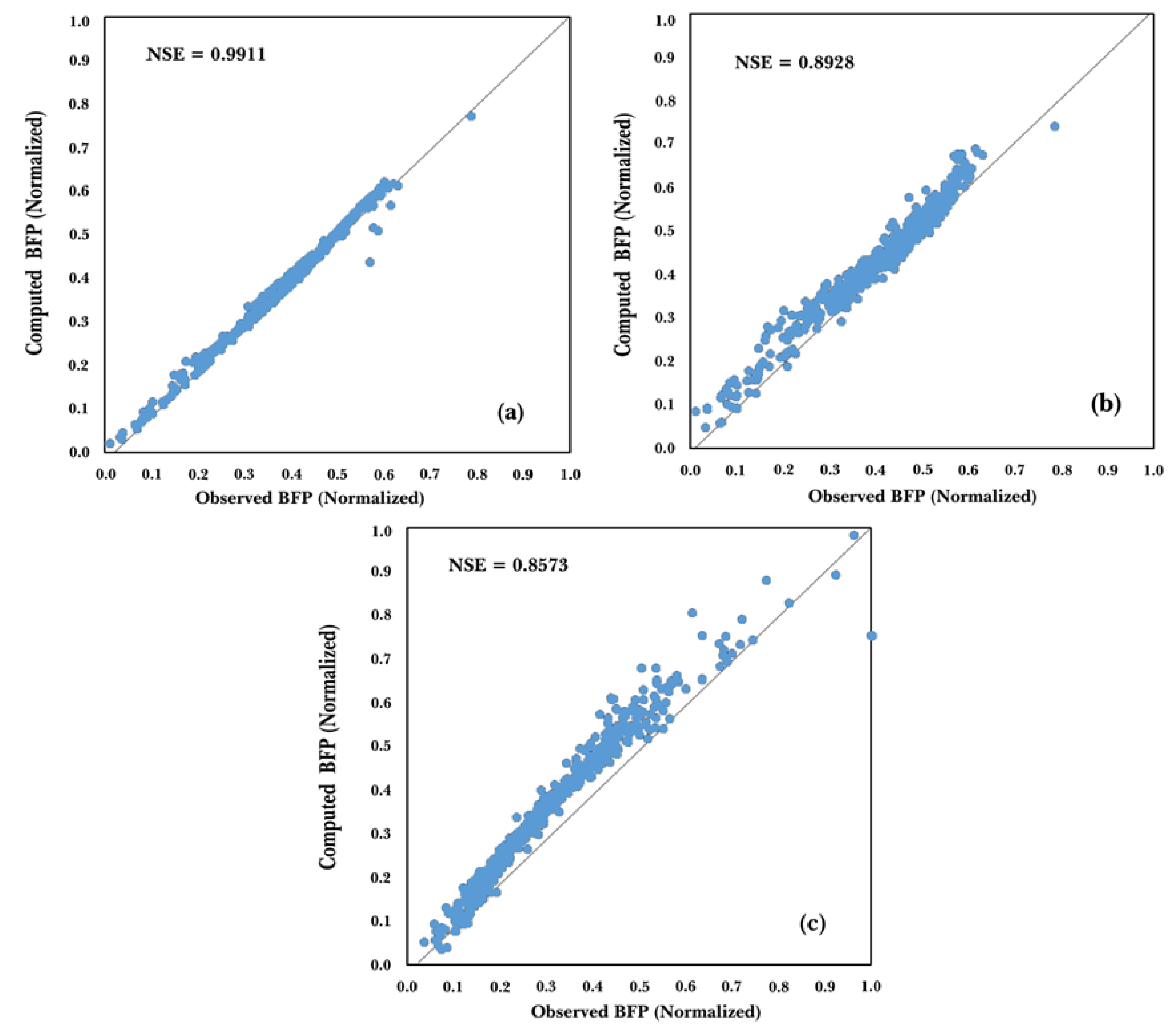
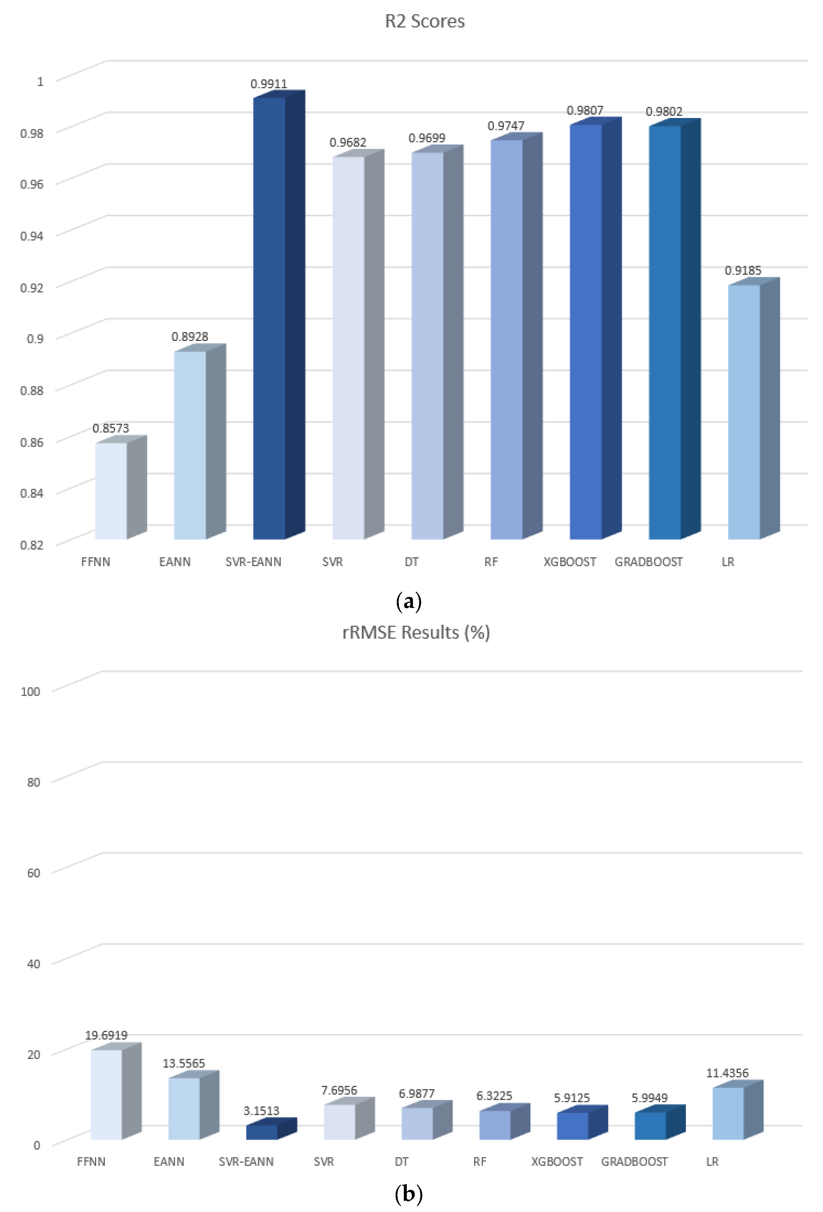
4.2. Regression Results and Comparisons

The EANN was trained as a predictor in the SVR-EANN hybrid model to achieve superior results for BFP prediction without considering the least significant factor determined by the SVR model. The age attribute was removed for SVR-EANN during the training, and the obtained results of the proposed SVR-EANN hybrid model were compared to the results of other benchmark models: feed-forward NN [36], SVR [29], DT [37], RF [38], LR [39], XGBoost [40], and GradBoost [41].

The network structure of the FFNN included an input layer, a single hidden layer with 20 neurons, and an output layer with a single neuron. The determination of the hidden neuron numbers was based on the training of the FFNN using a hidden neuron interval of 5–30 and epochs 10–1000. The highest result was obtained using 20 hidden neurons and 50 epochs with the Adam optimizer.

DT was implemented using mean squared error (MSE) criteria for constructing the DT for regression studies. GradBoost and RF were trained with 100 and 150 estimators, respectively. The learning rates of XGBoost and GradBoost were defined as 0.3 and 0.085. The number of estimators and the learning rates of RF, GradBoost, and XGBoost were determined after several trial-and-error experiments by validating the results using 4-fold cross-validation.

The final parameters of SVR were considered the same as the proposed hybrid model, and C, γ, and ε values were set to 5, 0.0313, and 0.25, respectively. The EANN was considered with twenty hidden and five hormone neurons and trained 50 epochs after searching the parameters similar to the FFNN search.

SVR-EANN achieved superior results by obtaining 0.991, 0.0125, and 3.15% R², RMSE, and rRMSE results, while the EANN without left-out sensitivity analysis obtained 0.8928, 0.0464, and 13.55% R², RMSE, and rRMSE results. The difference between the results of SVR-EANN and EANN shows the importance of data selection and the efficiency of the SVR-EANN. On the other hand, the FFNN, with its superior architecture and parameters, obtained lower results since it achieved 0.857, 0.0622, and 19.69% R², RMSE, and rRMSE results.

LR obtained the R², RMSE, and rRMSE results of 0.918, 0.0396, and 11.43%, since SVR achieved 0.968, 0.024, and 7.69%. The DT (R² = 0.969, RMSE = 0.0216, rRMSE 6.98%) and tree-based ensemble models, RF (R² = 0.974, RMSE = 0.0198, rRMSE 6.32%), XGBoost (R² = 0.98, RMSE = 0.0178, rRMSE 5.91%), and GradBoost (R² = 0.98, RMSE = 0.0182, rRMSE 5.99%) achieved relatively higher results than other models; however, they could not out-perform the proposed SVR-EANN model.

Table 4. BFP prediction results.

Models	R2	RMSE	RRMSE (%)
FFNN	0.8573	0.0622	19.6919
EANN	0.8928	0.0464	13.5565
SVR-EANN	0.9911	0.0125	3.1513
SVR	0.9682	0.0245	7.6956
DT	0.9699	0.0216	6.9877
RF	0.9747	0.0198	6.3225
XGBOOST	0.9807	0.0178	5.9125
GRADBOOST	0.9802	0.0182	5.9949
LR	0.9185	0.0396	11.4356

presents all results of the models in the test stage obtained in this study. Figure 6 shows the regression line of the testing stage using a scatter plot of the EANN, FFNN, and the proposed SVR-EANN.

4.3. Discussion

Detailed analysis of models based on machine learning modeling approaches is described in the previous section. All machine learning models were capable of predicting BFP using the considered primary dataset; however, the proposed SVR-EANN outperformed other models by achieving superior results for all evaluation metrics used in this study. In this section, the results of real data analytics are analogized with the literature.

There were several studies in the literature in the context of BFP prediction using ML algorithms. Apart from basic information and anthropometric measurements such as gender, age, BMI, height, weight, and waist circumference, single-stage intelligent predictors such as ANN and/or SVR were used to forecast BFP [1,8,9]. System performance in these studies varied between 44% and 80.43%. However, these studies included random selection of parameters and, nevertheless, could identify the most significant parameters to reach the best predictor variables. On the other hand, studies with hybrid machine learning in BFP prediction were proposed. These models contain a feature selection model that varies between the intelligence-based or statistic-based models to identify the most explanatory variables for the intelligent forecasting algorithm phase.

A model based on multiple regression (MR) and multivariate adaptive regression splines (MARSs) was employed in [11] to choose the best variables in the explanatory phase which resulted in two sets with five and six variables among 13 anthropometric parameters for the MR and MARSs, respectively. The most relevant variables included age, height, weight, abdomen 2 circumference (waist circumference), forearm circumference, waist circumference, thigh circumference, and neck circumference. In contrast, when ANN and SVR were utilized for BFP prediction, the MR-SVR achieved the best performance with an RMSE of 4.6427.

Hybrid models proposed by Uçar [12] employed Spearman’s correlation coefficients and principal component analysis computations for the feature selection phase to obtain the most predictive feature group from 13 different subgroups of anthropometric measurements. The intelligent hybrid models were constructed from the MLFFNN, DT, and SVM algorithms. The most significant result was achieved through the hybrid model DT-SVM with one anthropometric measurement named abdomen 2 circumference (waist circumference) and an RMSE of 0.482. However, both hybrid studies [11,12] considered the dataset collected by Johnson [10] from 252 male participants. Therefore, the gender feature was not discussed. In addition, both studies could not achieve higher results as in this study in terms of prediction rates, even though the dataset size was considerably small.

According to studies in the literature, certain parameters are effective in the estimation of BFP. Gender is the most evident factor [42,43,44]. A common equation for men and women has been derived in several investigations [8,45].

Gender information is included in the dataset used in this study. In addition to gender, benchmark studies on ML and BFP prediction with single or hybrid intelligent algorithms indicated the relative importance of other features such as BMI [1] and waist circumference [8,10,11]. However, to the best of our knowledge, this study is the first in clearly identifying the most significant parameter’s base in the intelligent model for BFP prediction. Parameters abdominal C (waist circumference) followed by gender were determined as the first and second most influential variables in the list of optimal parameters that affect BFP prediction indicated by the SVR sensitivity analysis.

In this study, all machine learning models were capable of predicting BFP using the considered primary dataset of 2000 people; however, the proposed hybrid model SVR-EANN with an intelligence-based feature selection algorithm outperformed other models by achieving superior results for all evaluation metrics used in this research. It was observed that selected data provide more accurate results than complete data, and it increased the prediction rates from 2.8% to 16% compared to other models. This showed that SVR could be used for regression tasks and data selection quite effectively. In addition to the success of SVR in data selection, it has been observed that the EANN, which is a new generation artificial neural network, achieves the highest results with appropriate data by imposing the hormone neurons that improve the learning ability.

The obtained results demonstrate the efficacy of the proposed hybrid SVR-EANN model for BFP. Furthermore, combining the efficiency of the two models, SVR-EANN showed that the hybrid models increase the probability of achieving superior results than conventional and single models. Figure 7 presents the visualization of the obtained R² scores and rRMSE results to demonstrate the differences between the models effectively. The highest and lowest indicators in the R² score and rRMSE results represent the superior prediction rates, respectively. However, the proposed model was not applied in different fields and disciplines, which is the study’s limitation.

5. Conclusions

Body fat percentage is a crucial indicator of human body health and requires a reliable and cost-effective prediction on a comprehensive dataset to provide experts information to take precautions, particularly for obesity. Body fat percentage calculation is rough and expensive, and hence efficient and cost-effective approaches are necessary. A large economic expansion is possible when the developed ML technologies are virtually applicable.

This paper released a primary dataset for body fat percentage prediction and proposed a hybrid machine learning model based on support vector regression and emotional neural networks to predict body fat percentage accurately. The SVR sensitivity analysis was combined with the prediction ability of emotional artificial neural networks in the hybrid model. The proposed SVR-EANN model was compared to seven benchmark machine learning models, and the results show that the SVR-EANN was superior to the others in all evaluation metrics considered in the study.

Our study demonstrated the importance of using SVR in feature selection for datasets with limited properties and measurements for BFP and how the regression ability could be improved using the EANN in a hybrid model. In addition, the consideration of benchmark ML models for comparison showed how the regression abilities of the models might differ from each other for BFP prediction studies and might lead to further ML studies on BFP.

In addition, the proposed hybrid model was used to determine the attributes affecting body fat percentage prediction. The results show that abdominal C has the most significant influence on body fat percentage. In contrast, the age attribute has the most negligible influence and could be ignored during prediction studies.

Our future work will include the prediction of body fat percentage using the proposed hybrid model within optical data and the investigation of gender effect on BFP. In addition, further experiments will be performed to analyze the efficiency of the suggested hybrid model in the prediction of body fat percentage in obese children.

References

1. Kupusinac, A.; Stokić, E.; Doroslovački, R. Predicting body fat percentage based on gender, age and BMI by using artificial neural networks. Comput. Methods Programs Biomed. 2014, 113, 610–619. [Google Scholar] [CrossRef]
2. Fan, J.-G.; Kim, S.-U.; Wong, V.W.-S. New trends on obesity and NAFLD in Asia. J. Hepatol. 2017, 67, 862–873. [Google Scholar] [CrossRef] [Green Version]
3. Flegal, K.M.; Shepherd, J.A.; Looker, A.C.; Graubard, B.I.; Borrud, L.G.; Ogden, C.L.; Harris, T.B.; Everhart, J.E.; Schenker, N. Comparisons of percentage body fat, body mass index, waist circumference, and waist-stature ratio in adults. Am. J. Clin. Nutr. 2009, 89, 500–508. [Google Scholar] [CrossRef]
4. Swainson, M.G.; Batterham, A.M.; Tsakirides, C.; Rutherford, Z.H.; Hind, K. Prediction of whole-body fat percentage and visceral adipose tissue mass from five anthropometric variables. PLoS ONE 2017, 12, e0177175. [Google Scholar] [CrossRef]
5. DeGregory, K.; Kuiper, P.; DeSilvio, T.; Pleuss, J.; Miller, R.; Roginski, J.; Fisher, C.; Harness, D.; Viswanath, S.; Heymsfield, S. A review of machine learning in obesity. Obes. Rev. 2018, 19, 668–685. [Google Scholar] [CrossRef]
6. Chen, W.; Hou, X.-H.; Zhang, M.-L.; Bao, Y.-Q.; Zou, Y.-H.; Zhong, W.-H.; Xiang, K.-S.; Jia, W.-P. Comparison of body mass index with body fat percentage in the evaluation of obesity in Chinese. Biomed. Environ. Sci. 2010, 23, 173–179. [Google Scholar] [CrossRef]
7. Sekeroglu, B.; Tuncal, K. Prediction of cancer incidence rates for the European continent using machine learning models. Health Inform. J. 2021, 27. [Google Scholar] [CrossRef]
8. Ferenci, T.; Kovacs, L. Predicting body fat percentage from anthropometric and laboratory measurements using artificial neural networks. Appl. Soft Comput. 2018, 67, 834–839. [Google Scholar] [CrossRef]
9. Chiong, R.; Fan, Z.; Hu, Z.; Chiong, F. Using an improved relative error support vector machine for body fat prediction. Comput. Methods Programs Biomed. 2021, 198, 105749. [Google Scholar] [CrossRef]
10. Johnson, R.W. Fitting percentage of body fat to simple body measurements. J. Stat. Educ. 1996, 4. [Google Scholar] [CrossRef]
11. Shao, Y.E. Body fat percentage prediction using intelligent hybrid approaches. Sci. World J. 2014, 2014. [Google Scholar] [CrossRef] [Green Version]
12. Uçar, M.K.; Ucar, Z.; Köksal, F.; Daldal, N. Estimation of body fat percentage using hybrid machine learning algorithms. Measurement 2021, 167, 108173. [Google Scholar] [CrossRef]
13. Liu, M.; Chen, L.; Du, X.; Jin, L. Activated Gradients for Deep Neural Networks. IEEE Trans. Neural Netw. Learn. Syst. 2021, 1–13. [Google Scholar] [CrossRef]
14. Khashman, A. A modified backpropagation learning algorithm with added emotional coefficients. IEEE Trans. Neural Netw. 2008, 19, 1896–1909. [Google Scholar] [CrossRef]
15. Rahman, M.A.; Milasi, R.M.; Lucas, C.; Araabi, B.N.; Radwan, T.S. Implementation of emotional controller for interior permanent-magnet synchronous motor drive. IEEE Trans. Ind. Appl. 2008, 44, 1466–1476. [Google Scholar] [CrossRef]
16. Nourani, V. An emotional ANN (EANN) approach to modeling rainfall-runoff process. J. Hydrol. 2017, 544, 267–277. [Google Scholar] [CrossRef]
17. Gholami, A.; Bonakdari, H.; Samui, P.; Mohammadian, M.; Gharabaghi, B. Predicting stable alluvial channel profiles using emotional artificial neural networks. Appl. Soft Comput. 2019, 78, 420–437. [Google Scholar] [CrossRef]
18. Sharghi, E.; Nourani, V.; Najafi, H.; Gokcekus, H. Conjunction of a newly proposed emotional ANN (EANN) and wavelet transform for suspended sediment load modeling. Water Supply 2019, 19, 1726–1734. [Google Scholar] [CrossRef]
19. Biswas, R.; Samui, P.; Rai, B. Determination of compressive strength using relevance vector machine and emotional neural network. Asian J. Civ. Eng. 2019, 20, 1109–1118. [Google Scholar] [CrossRef]
20. De Koning, L.; Merchant, A.T.; Pogue, J.; Anand, S.S. Waist circumference and waist-to-hip ratio as predictors of cardiovascular events: Meta-regression analysis of prospective studies. Eur. Heart J. 2007, 28, 850–856. [Google Scholar] [CrossRef]
21. Usman, A.; Işik, S.; Abba, S. A novel multi-model data-driven ensemble technique for the prediction of retention factor in HPLC method development. Chromatographia 2020, 83, 933–945. [Google Scholar] [CrossRef]
22. Cavus, N.; Mohammed, Y.B.; Yakubu, M.N. Determinants of Learning Management Systems during COVID-19 Pandemic for Sustainable Education. Sustainability 2021, 13, 5189. [Google Scholar] [CrossRef]
23. Khashman, A. Neural networks for credit risk evaluation: Investigation of different neural models and learning schemes. Expert Syst. Appl. 2010, 37, 6233–6239. [Google Scholar] [CrossRef]
24. Ozsahin, I.; Sekeroglu, B.; Mok, G.S. The use of back propagation neural networks and 18F-Florbetapir PET for early detection of Alzheimer’s disease using Alzheimer’s Disease Neuroimaging Initiative database. PLoS ONE 2019, 14, e0226577. [Google Scholar] [CrossRef] [Green Version]
25. Kumar, P.; Nigam, S.; Kumar, N. Vehicular traffic noise modeling using artificial neural network approach. Transp. Res. Part C Emerg. Technol. 2014, 40, 111–122. [Google Scholar] [CrossRef]
26. Nourani, V.; Alami, M.T.; Vousoughi, F.D. Wavelet-entropy data pre-processing approach for ANN-based groundwater level modeling. J. Hydrol. 2015, 524, 255–269. [Google Scholar] [CrossRef]
27. Nourani, V.; Gökçekuş, H.; Umar, I.K.; Najafi, H. An emotional artificial neural network for prediction of vehicular traffic noise. Sci. Total. Environ. 2020, 707, 136134. [Google Scholar] [CrossRef]
28. Vapnik, V.N. Statistical Learning Theory; Haykin, S., Ed.; Wiley: New York, NY, USA, 1998. [Google Scholar]
29. Cavus, N.; Mohammed, Y.B.; Yakubu, M.N. An Artificial Intelligence-Based Model for Prediction of Parameters Affecting Sustainable Growth of Mobile Banking Apps. Sustainability 2021, 13, 6206. [Google Scholar] [CrossRef]
30. Wang, W.-c.; Xu, D.-m.; Chau, K.-w.; Chen, S. Improved annual rainfall-runoff forecasting using PSO–SVM model based on EEMD. J. Hydroinform. 2013, 15, 1377–1390. [Google Scholar] [CrossRef]
31. Oytun, M.; Tinazci, C.; Sekeroglu, B.; Acikada, C.; Yavuz, H.U. Performance prediction and evaluation in female handball players using machine learning models. IEEE Access 2020, 8, 116321–116335. [Google Scholar] [CrossRef]
32. Nourani, V.; Gökçekuş, H.; Umar, I.K. Artificial intelligence based ensemble model for prediction of vehicular traffic noise. Environ. Res. 2020, 180, 108852. [Google Scholar] [CrossRef]
33. Rabehi, A.; Guermoui, M.; Lalmi, D. Hybrid models for global solar radiation prediction: A case study. Int. J. Ambient. Energy 2020, 41, 31–40. [Google Scholar] [CrossRef]
34. Hsu, C.-W.; Chang, C.-C.; Lin, C.-J. A Practical Guide to Support Vector Classification; National Taiwan University: Taipei, Taiwan, 2003. Available online: http://www.csie.ntu.edu.tw/~cjlin/papers.html (accessed on 14 October 2021).
35. Nourani, V.; Elkiran, G.; Abdullahi, J.; Tahsin, A. Multi-region modeling of daily global solar radiation with artificial intelligence ensemble. Nat. Resour. Res. 2019, 28, 1217–1238. [Google Scholar] [CrossRef]
36. Rumelhart, D.E.; Hinton, G.E.; Williams, R.J. Learning representations by back-propagating errors. Nature 1986, 323, 533–536. [Google Scholar] [CrossRef]
37. Loh, W.Y. Classification and regression trees. Wiley Interdiscip. Rev. Data Min. Knowl. Discov. 2011, 1, 14–23. [Google Scholar] [CrossRef]
38. Zhang, C.; Li, Y.; Yu, Z.; Tian, F. Feature selection of power system transient stability assessment based on random forest and recursive feature elimination. In Proceedings of the 2016 IEEE PES Asia-Pacific Power and Energy Engineering Conference (APPEEC), Xi’an, China, 25–28 October 2016; pp. 1264–1268. [Google Scholar] [CrossRef]
39. Stanton, J.M. Galton, Pearson, and the peas: A brief history of linear regression for statistics instructors. J. Stat. Educ. 2001, 9. [Google Scholar] [CrossRef]
40. Chen, T.; Guestrin, C. Xgboost: A scalable tree boosting system. In Proceedings of the 22nd ACM SIGKDD International Conference on Knowledge Discovery and Data Mining, San Francisco, CA, USA, 13–17 August 2016; pp. 785–794. [Google Scholar] [CrossRef] [Green Version]
41. Friedman, J.H. Greedy function approximation: A gradient boosting machine. Ann. Stat. 2001, 1189–1232. [Google Scholar] [CrossRef]
42. Stevens, J.; Truesdale, K.P.; Cai, J.; Ou, F.-S.; Reynolds, K.R.; Heymsfield, S.B. Nationally representative equations that include resistance and reactance for the prediction of percent body fat in Americans. Int. J. Obes. 2017, 41, 1669–1675. [Google Scholar] [CrossRef] [Green Version]
43. Leahy, S.; O’Neill, C.; Sohun, R.; Toomey, C.; Jakeman, P. Generalised equations for the prediction of percentage body fat by anthropometry in adult men and women aged 18–81 years. Br. J. Nutr. 2013, 109, 678–685. [Google Scholar] [CrossRef] [Green Version]
44. Deurenberg, P.; Deurenberg-Yap, M.; Wang, J.; Lin, F.P.; Schmidt, G. Prediction of percentage body fat from anthropometry and bioelectrical impedance in Singaporean and Beijing Chinese. Asia Pac. J. Clin. Nutr. 2000, 9, 93–98. [Google Scholar] [CrossRef]
45. Fthenakis, Z.G.; Balaska, D.; Zafiropulos, V. Uncovering the FUTREX-6100XL prediction equation for the percentage body fat. J. Med. Eng. Technol. 2012, 36, 351–357. [Google Scholar] [CrossRef]
Figure 1. Plot of correlation matrix between the variables.
Applsci 11 09797 g001
Figure 2. A node of EANN and emotional unit [16].
Applsci 11 09797 g002
Figure 3. Conceptual structure of SVR model [31].
Applsci 11 09797 g003
Figure 4. Algorithm for SVR left-out sensitivity analysis.
Applsci 11 09797 g004
Figure 5. Block diagram of the proposed SVR-EANN hybrid model.
Applsci 11 09797 g005
Figure 6. Scatter plots of the testing stage for predicted BFP: (a) SVR-EANN, (b) EANN, (c) FFNN.
Applsci 11 09797 g006
Figure 7. Visualization of the results obtained in this study, (a) R2 scores, and (b) rRMSE results.
Applsci 11 09797 g007