Article

Dynamic Stall Characteristics of the Bionic Airfoil with Different Waviness Ratios

School of Energy and Power Engineering, Xi’an Jiao Tong University, Xian Ning West Road, Xi’an 710049, China
*
Author to whom correspondence should be addressed.
Appl. Sci. 2021, 11(21), 9943; https://doi.org/10.3390/app11219943
Submission received: 2 September 2021 / Revised: 1 October 2021 / Accepted: 20 October 2021 / Published: 25 October 2021

Abstract

:
A dynamic stall will cause dramatic changes in the aerodynamic performance of the blade, resulting in a sharp increase in the blade vibration load. The bionic leading-edge airfoil with different waviness ratios, inspired by the humpback whales flipper, is adopted to solve this problem. In this study, based on the NACA0015 airfoil, the three-dimensional unsteady numerical simulation and sliding mesh technique are used to reveal the flow control mechanism on the dynamic stall of the bionic wavy leading edge. The effects of the waviness ratio on the dynamic stall characteristics of the airfoil are also investigated. The results show that the peak drag coefficient is dramatically reduced when a sinusoidal leading edge is applied to the airfoil. Although the peak lift coefficient is also reduced, the reduction is much smaller. When the waviness ratio R is 0.8, the peak drag coefficient of the airfoil is reduced by 17.14% and the peak lift coefficient of the airfoil is reduced by 9.20%. The dynamic hysteresis effect is improved gradually with an increasing waviness ratio. For the bionic airfoil with R = 1.0, the area of the hysteresis loop is the smallest.

1. Introduction

On jet engine compressor blades, wind turbines, maneuvering fixed-wing aircrafts, and helicopter rotor blades, dynamic stall can occur and can become the main factor limiting performance [1,2]. Consequently, it is essential to develop methods for the control of flow separation. Flow control techniques can be applied to improve the aerodynamic performance of the airfoil, thereby leading to improvements in civil and military aviation economics. A variety of flow control techniques have been investigated in both academia and industry [3], including synthetic jets [4] and vortex generators [5].
Recent developments in bionic technology [6,7] have inspired engineers to investigate its application in many areas, such as in drag reduction [8], robot design [9], and aircraft design [10,11]. One biomimetic concept has attracted particular attention, namely the tubercles on the pectoral fins of humpback whales. These tubercles play a role as flow control devices to improve hydrodynamic performance [12]. Miklosovic et al. [13] were among the first to study the aerodynamic effects of the leading-edge tubercles of humpback whale flippers. They found that the stall angle of the model, modified by leading-edge tubercles, was increased by 40% and the drag in the post-stall region was reduced. Pérez-Torró and Kim [14] conducted a numerical study of the effect of a sinusoidal wavy tubercle edge on the NACA 0021 airfoil at a low Reynolds number. It was observed that laminar separation bubbles (LSBs) were formed in a collocated fashion in the trough area of the wavy leading edge rather than being periodically or uniformly distributed over the span. Serson et al. [15] investigated the performance of a NACA 0012 airfoil with a sinusoidal convex leading edge through direct numerical simulation at Re = 1000. The results indicated that the waviness reduced the lift–drag ratio for this value of Re and that this reduction was associated with the suppression of the lift coefficient fluctuation. Hansen et al. [16] carried out an experimental investigation to determine the influence of leading sinusoidal protrusions on two different NACA airfoils. For both airfoils, reducing the tubercle amplitude led to a larger stall angle and a higher maximum lift coefficient. The results also suggested that tubercles act similarly to conventional vortex generators. Yoon et al. [17] numerically investigated the effect of the wavy leading edge on the hydrodynamic characteristics of three-dimensional wings. They also suggested that the wavy leading-edge tubercle acts as a vortex generator. In addition, Cai et al. [18] provided a necessary perspective for an overall understanding of the mechanism of flow modification by multiple leading-edge protrusions. Flores Mezarina et al. [19] adopted, as a new parameter for leading-edge protrusion, the asymmetry factor, which determines the peak position along the wavelength direction of the tubercle. Wind tunnel and visualization tests demonstrated that an asymmetric protuberance directly influences the spanwise flow and induces resistance. Kant and Bhattacharyya [20] studied the hydrodynamic characteristics of a new type of hydrofoil modified by a twin protuberance. Compared with the baseline hydrofoil, the lift coefficient and maximum lift of the modified foil decreased before stalling, but the lift coefficient was higher after stalling. Fish and Lauder [21] reviewed both active and passive flow control methods adopted by swimming fish and mammals, and considered numerical and experimental studies of the static aerodynamic characteristics of airfoils, in this context, dating from 1995 to 2004. They concluded that wavy leading-edge tubercles could increase lift and reduce drag.
The above studies were all concerned about how a wavy leading edge affected the static characteristics of airfoils. However, we should also consider the effect of the wavy tubercle edge on the dynamic stall characteristics of airfoils.
The effects of a wavy leading edge on a pitching NACA 0018 profile were investigated experimentally and numerically by Rohmawati et al. [22]. They found that the increase in lift on the upstroke was higher than that on the downstroke. Additionally, the increase in drag was less than the increase in lift. These numerical simulation results showed that stall is suppressed during the pitching motion of the wing. The static and dynamic characters of a NACA 634-021 airfoil with the sinusoidal leading edge were numerically simulated by Cai et al. [23] using the Spalart–Allmaras (S-A) turbulence model. For dynamic stall, the results showed that the aerodynamic performance of the modified airfoil was stable at a high angle of attack, which resulted in a reduction in the area of the lift coefficient hysteresis loop. Hrynuk and Bohl [24] experimentally studied the effect of a wavy tubercle edge, inspired by humpback flippers, on the dynamic performance of an airfoil at angles of attack from 0° to 50°. Their results showed that the leading-edge tubercles on the flippers acted as a passive flow control mechanism controlling or delaying dynamic stall. Aftab et al. [25] presented a comprehensive review of recent research on wavy leading edges. Related experimental and numerical results show that the flow pattern of the wave-shaped front edge structure is entirely different from that of the traditional airfoil. In addition, the leading edge of the nodule can solve aerodynamic problems such as flow separation, noise, and dynamic stall. This review described research on different airfoils and the performance improvements that had been obtained. It also summarized the main contributions of previous studies and identified their shortcomings. The influence of a tubercle leading edge on dynamic stall characteristics was described. Choudhry et al. [26] presented a detailed review of experimental studies of dynamic stall. They discussed the effects of various parameters, such as reduced frequency, Reynolds number, Mach number, and airfoil geometry, on dynamic stall characteristics. As Anders [27] emphasized, although research on the front structure has been carried out for many years, there is still a need for further research on this topic.
From the literature review presented above, the effects of leading-edge protuberance on the static and dynamic aerodynamic performance of the airfoil have been studied numerically and experimentally. The airfoil with a wavy leading edge can maintain a high lift in the static stall by delaying the stall. In the case of a dynamic stall, a wavy leading edge can suppress the dynamic stall hysteresis of the airfoil. However, there have been few reports on the effects of wavy leading edges with different waviness ratios on the dynamic stall performance of airfoils. Thus, the dynamic stall characteristics of the airfoils with varying ratios of waviness are investigated in the present research study. The force coefficients, instantaneous flow patterns, and pressure distribution are obtained and compared with those of the conventional NACA 0015 airfoil. The flow control mechanism of the wavy leading edge of the airfoil is revealed based on the numerical results. This study expects to provide a valuable reference for improving the performance of aircraft and impeller machinery through the optimal design of the blade.

2. Materials and Methods

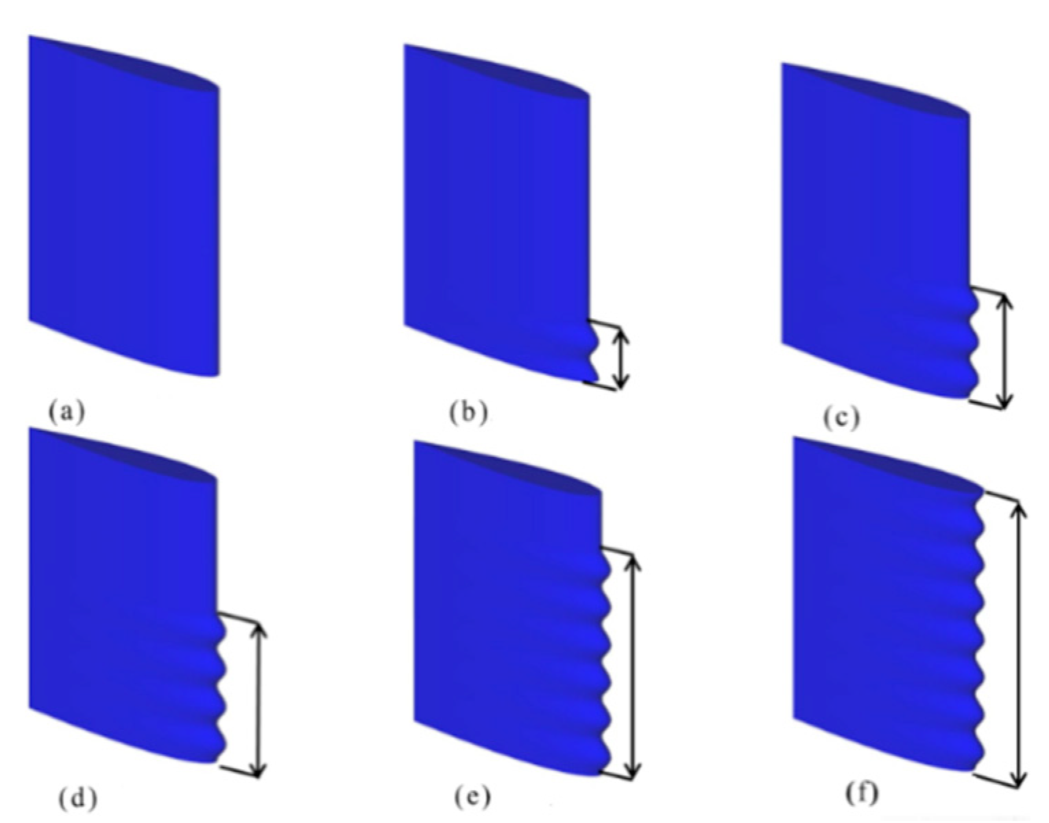
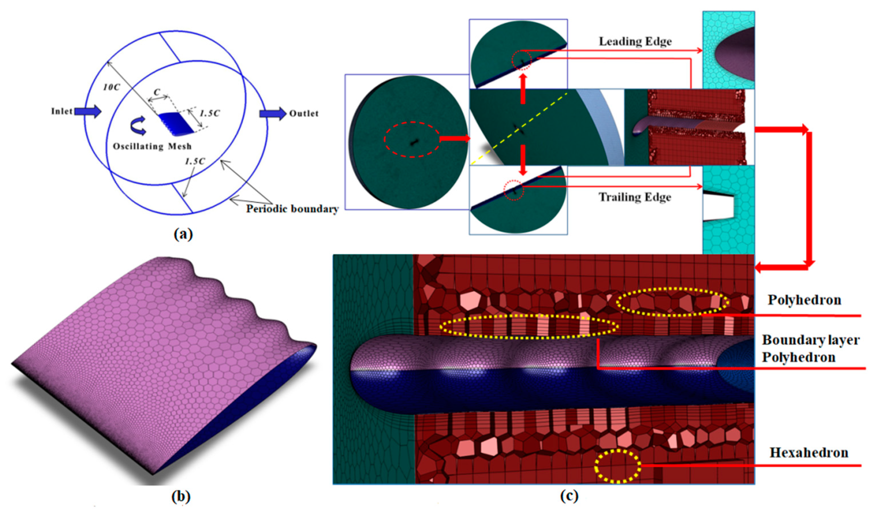
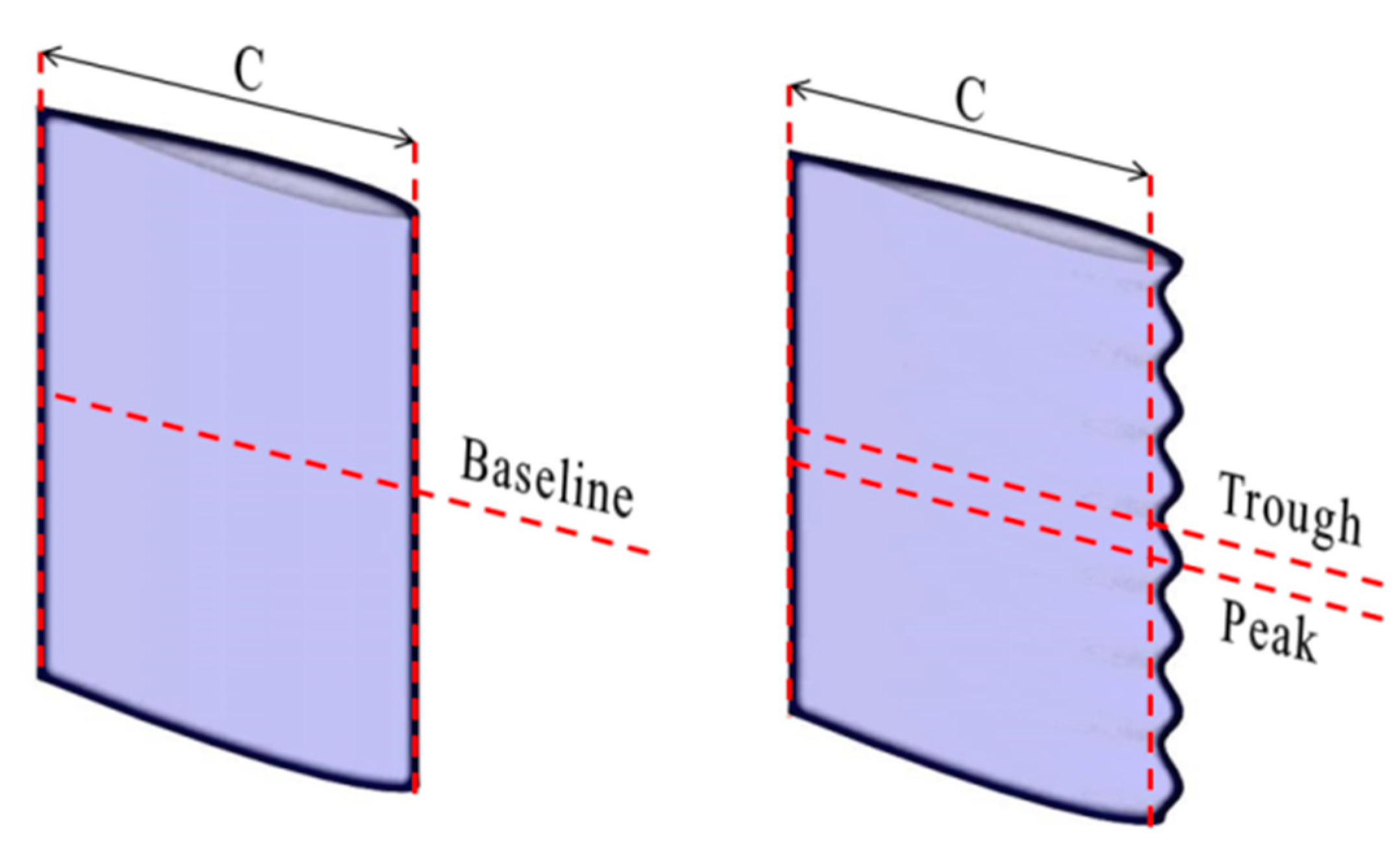
2.1. The Geometric Model and Grids

The humpback whales have pectoral fins with leading-edge tubercles (Figure 1). Due to these tubercles, humpback whales are significantly more mobile than other mammals and a unique way of rotary predation is formed.
The wavy leading edge in the spanwise is described by Equation (1).
C ( z ) = C + a 2 [ 1 + c o s ( 2 π z λ ) ]
where C(z) is the local chord length of the airfoil, a is the wavy amplitude, and λ is the wavelength. In the present research study, the wavy amplitude is 0.025 C and the wavelength is 0.2 C. C is the chord length.
The purpose of this study was to numerically investigate the effect of the wavy leading edge on the dynamic aerodynamic characteristics of the three-dimensional viscous flow around a low aspect ratio airfoil. The aspect ratio of 1.5 belongs to the proportion range of the wing of the micro air vehicles. Therefore, the airfoil aspect ratio (AR) is denoted by AR= S / C =1.5 and the waviness ratio (R) is represented by R= SW, where S. S is the span of an airfoil and Sw is the span of waviness. According to the literature [17], we studied the aerodynamic characteristics of the airflow around the wavy wing with five different waviness ratios (0.2, 0.4, 0.6, 0.8, and 1.0). The schematics of the baseline airfoil and wavy airfoil with five waviness ratios are shown in Figure 2.
Figure 3a is a schematic of the computational domain and boundary conditions. The size of the calculation domain forming a cylindrical shape was defined by a radius of 10 C and a height of 1.5 C. The inlet and outlet boundaries were 10 C from the airfoil surface to avoid the boundary reflections, while the far-field boundary was set as the periodic boundary. In this case, the velocity inlet was set to 22 m/s and the pressure outlet was set as free-stream pressure. As shown in Figure 3b,c, an unstructured grid arrangement was used. A no-slip boundary condition was applied to the airfoil surface. When using the SST k-ω turbulence model, it was necessary to control the height of the grid perpendicular to the wall direction so that the wall nodes were in the viscous sublayer and y+ < 1.0. Consequently, these grid distributions were generated such that the y+ in the first layer of the grids adjacent to the airfoil surface was kept near 1.

2.2. The Law of the Oscillating Airfoil

The NACA0012 and NACA0015 airfoils were used for numerical calculation verification. The NACA0012 airfoil oscillates sinusoidally and periodically around a chord length of 1/4 in the range of −5°~25° according to the law of Equation (2)
α ( t ) = α m e a n + α a m p sin ( 2 π f t )
The NACA0015 airfoil oscillates in pitch at about the one-quarter chord length location in the range of 0°~20° according to Equation (3)
α ( t ) = α mean α amp cos ( 2 π f t )
In Equations (2) and (3), αmean, αamp, and f are the mean angle of attack (AOA), pitch oscillation amplitude, and oscillation frequency, respectively. Their values are presented in Table 1.

2.3. Control Equation and Turbulence Model

In the numerical simulation case, the fluid flow was considered to be a viscous incompressible turbulent flow. The density of the fluid was constant. The flow control equations are the continuity Equation (4)
ρ t + x i ( ρ u i ) = 0
and the momentum Equation (5)
t ( ρ u i ) + x j ( ρ u i u j ) = p x i + x j [ μ ( u i x j + u j x i 2 3 δ i j u l x l ) ] + x j ( ρ u i u j ¯ )
where t and xi are time and space in Cartesian coordinates; p, ρ, and ν are the time-averaged pressure, density, and kinematic viscosity; and ρ u i u j ¯ is the Reynolds stress.
The URANS equations are solved based on the finite volume method. For the turbulent flow calculations, the SST k-ω turbulence model was chosen due to its ability to capture dynamic flow structures in a wide range of Reynolds numbers [28].
The SST k-ω turbulence model is a two-equation eddy viscosity model. The turbulent kinetic energy transport k is governed by Equation (6).
t ( ρ k ) + x j [ ρ u j k ( μ + σ k μ t ) k x j ] = τ t i j S i j β * ρ ω k
The equation for the specific consumption rate ω is Equation (7).
t ( ρ ω ) + x j [ ρ u j k ( μ + σ ω μ t ) ω x j ] = P ω β ρ ω 2 + 2 ( 1 F 1 ) ρ σ ω 2 ω k ω x j x j
The eddy viscosity model for the Reynolds stress is Equation (8).
τ t i j = 2 μ t ( S i j 1 3 S n m δ i j ) 2 3 ρ k δ i j
The function F1 is given by Equation (9).
{ F 1 = tanh Φ 1 4 Φ 1 = min [ max ( k 0.09 ω y , 500 μ ρ y 2 ω ) , 4 ρ k σ ω 2 D ω + y 2 ] D ω + = max ( 2 ρ 1 σ ω 2 1 ω k x j ω x j , 10 10 )
In the equation system(9), y is the distance to the next surface and Dω+ is the positive part of the cross-diffusion term. μt =ρ k /ω is the eddy viscosity; Sij is the average velocity strain-rate tensor; β = 0.09, σk = 0.2, and σω = 0.2 are model constants; and δij is the Kronecker delta.

3. The Numerical Calculation Verification

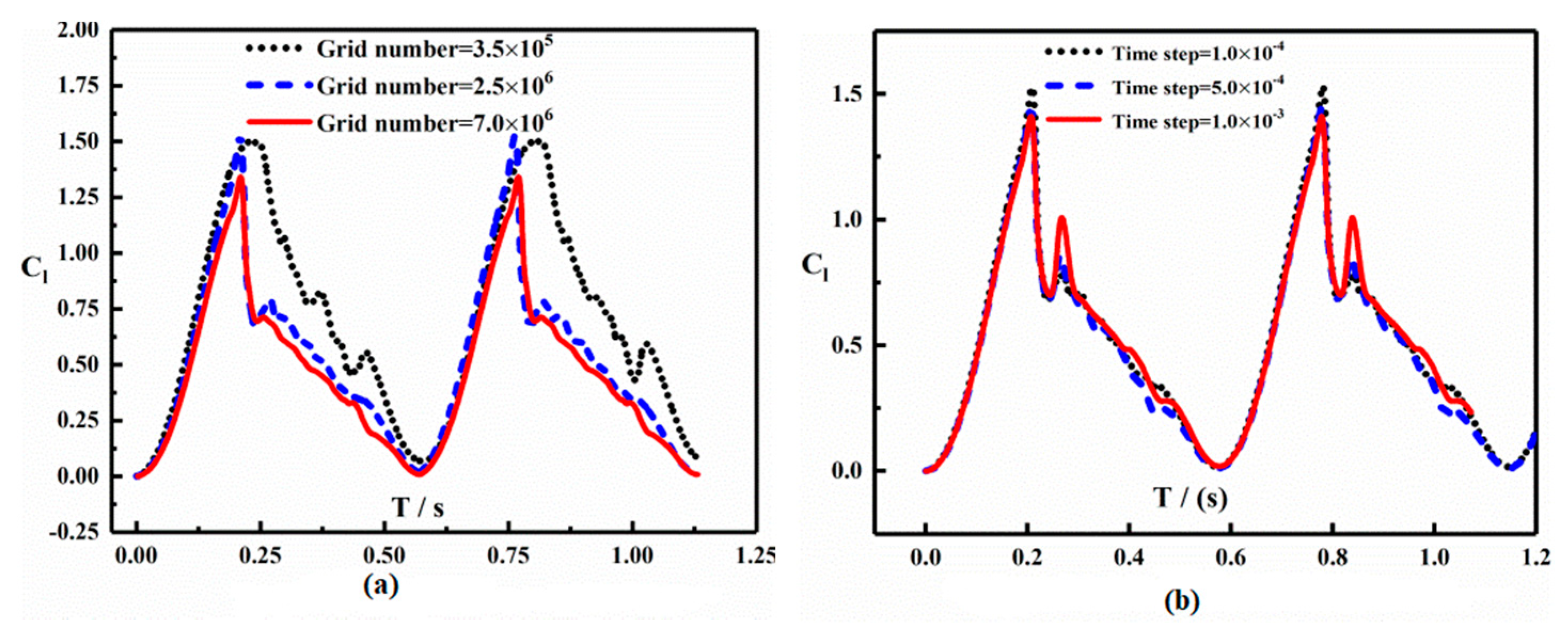
3.1. Sensitivity Analysis of Calculation Results

A grid and time-step sensitivity analysis of the computational domain was conducted to ensure the validity of the numerical calculation. In this paper, the grid independence was verified firstly. After determining the number of grids, the time-step independence was confirmed again.
A grid convergence analysis was performed for three different mesh distributions (coarse, medium, and fine), namely 3.5 × 10⁵, 2.5 × 10⁶, and 7.0 × 10⁶, as shown in Figure 4a. It can be seen that the results obtained from the medium and fine grids are in good agreement and establish a discrepancy with those from the coarse grid in terms of lift fluctuation and approximate period. Therefore, it can be considered that the grid independence of the solution was reached. The grid number of 2.5 × 10⁶ was selected for all subsequent calculations for reasons related to computational cost and computational efficiency. Three kinds of time steps (1.0 × 10⁻⁴ s, 5.0 × 10⁻⁴ s, and 1.0 × 10⁻³ s) were selected for the verification of time-step independence (Figure 4b). The lift coefficient varied periodically with time. It was also found that the lift coefficients were entirely consistent at the time steps of 1.0 × 10⁻⁴ s and 5.0 × 10⁻⁴ s, whereas the lift coefficient was slightly different at the time step of 1.0 × 10⁻³ s. In the following simulations, the time step of 5.0 × 10⁻⁴ s was selected.

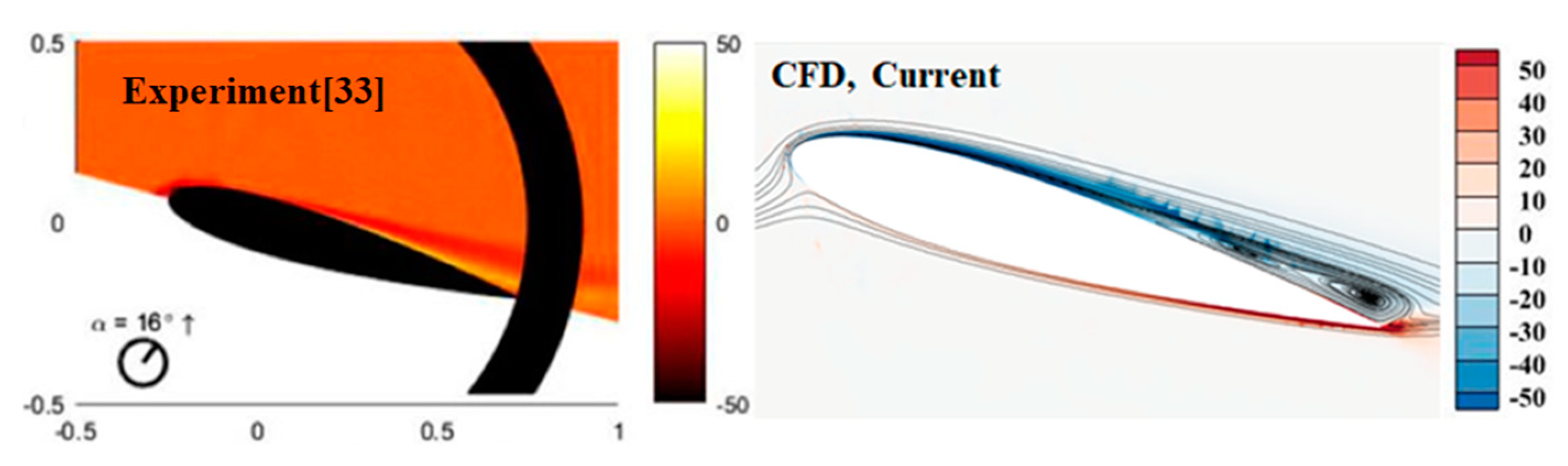
3.2. Numerical Simulation Validation

The results of the validation case are shown in Figure 5. The NACA0012 and NACA0015 airfoils were used for the numerical calculation verification and the results were compared with the corresponding experimental and numerical results. The primary flow conditions, Mach number, and other parameters of the calculation examples in this paper are consistent with the related wind tunnel tests.
In the upstroke stage (Figure 5a), the lift coefficient was consistent with the experimental [29] and numerical results [30,31], but in the downward (attack angle decreases) process, there was a deviation between the calculated results and the experimental values, which is related to the strong non-equilibrium of the separated turbulence. As the parameters in the turbulence model are often obtained by simple flow, however, in wind tunnel experiments, the measurement of the surface pressure at a high attenuation frequency will be very challenging due to the complex flow-field structure under deep stall (Kim and Xie [32]).
Figure 5b depicts the variation of the lift coefficient of the NACA0015 airfoil with the angle of attack during the dynamic stall. Additionally, it is compared with the experimental results of literature [33] and the 2D numerical simulation results of literature [34] using RSM and SST k-w models. The 3D numerical simulation calculations were used in this article. As shown in Figure 5b, the general trend of the lift curve calculated was consistent with the experimentally measured trend during most of the pitch cycle. The difference between the numerical simulation and the experiment of the lift coefficient is due to many factors. For example, the URANS method cannot faithfully resolve complex flows. The RSM and SST k-w methods produce almost the same results on the upstroke movement of the airfoil. The SST k-w model results in a smoother lift curve and more minor lift changes during the downstroke. Considering the complexity of dynamic stall, we judge that the results obtained using these two models are consistent.
The dynamic stall angle of the 3D numerical calculation results was slightly different from the experimental results, but the lift coefficient during the airfoil ascent phase was closer to the experimental value. Moreover, the results of the 3D simulation were qualitatively similar to the experimental results. The main flow structure was captured. Therefore, our simulation accuracy was considered acceptable because dynamic stalls and their controls are notoriously difficult to predict. Our work focuses on helping readers qualify the physics and control mechanisms of dynamic stalls rather than accurately solving dynamic stalls themselves.
To further verify the validity of the calculation results, the transient vorticity field from our simulation was compared with the phase-averaged flow field from the experiment [33]. The flow separation region and the vorticity of the airfoil suction surface can be seen in the flow visualizations in Figure 6, which were obtained from the numerical simulation and experimental observations. The close similarity between the experimental and simulated flow patterns can also be seen.
However, there were some differences between the numerical results and experimental results. The numerical method used in this paper can simulate dynamic stalls and capture relevant flow-field structures as well as flow details. The SST k-w model was used in all the simulations below.

4. Results and Analysis

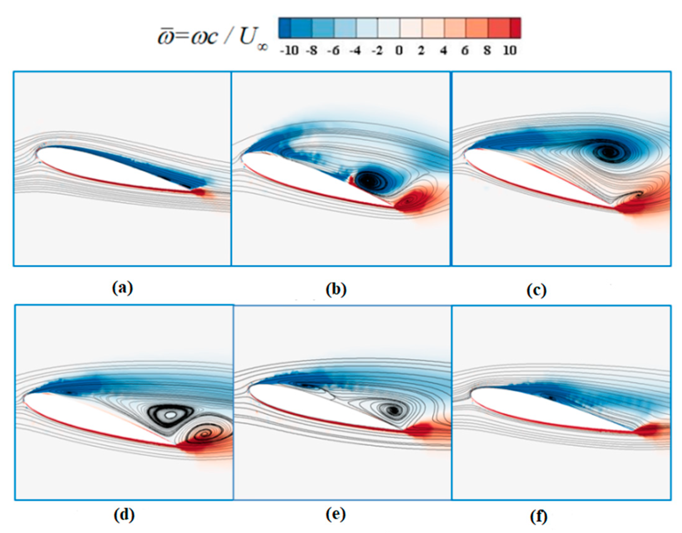
4.1. Flow Character of the Baseline Airfoil

To reveal the flow field of the baseline airfoil in the dynamic stall, the transient vorticity streamlines of the baseline airfoil at a typical moment in a pitching cycle are shown in Figure 7.
When the angle of attack was 14°, the airflow was completely attached to the airfoil surface and there was no flow separation (Figure 7a). The airflow at the trailing edge of the airfoil flowed back when the angle of attack increased. Next, the countercurrent increased rapidly and moved upstream. When the angle of attack reached 18°, two large-scale separation vortices were formed on the airfoil surface (Figure 7b). The lift decreased rapidly. When the angle of attack reached its maximum value of 20° and the flow on the upper surface of the airfoil was separated (Figure 7c). The airfoil then began to pitch down and it became completely stalled. Figure 7d–f show the detailed flow development in the final stage of the dynamic stall.
Figure 8 shows the vorticity–velocity iso-surface distributions of the baseline airfoil at several typical stages in the dynamic stall. Consistent with the flow trend of Figure 7, when the airfoil started to rise, the airflow was attached to its surface and no flow separation occurred on this surface. A backflow phenomenon began to appear at the tail of the airfoil, with the angle of attack gradually increasing. The backflow then gradually increased and flowed towards the leading edge of the airfoil. The surface of the airfoil exhibited a large-scale separation vortex (Figure 8b). When the airfoil reached the maximum angle of attack, the airflow on its surface was completely separated. The airfoil then started to move downward and the degree of flow separation on the airfoil surface gradually decreased, finally reaching a state of reattachment.

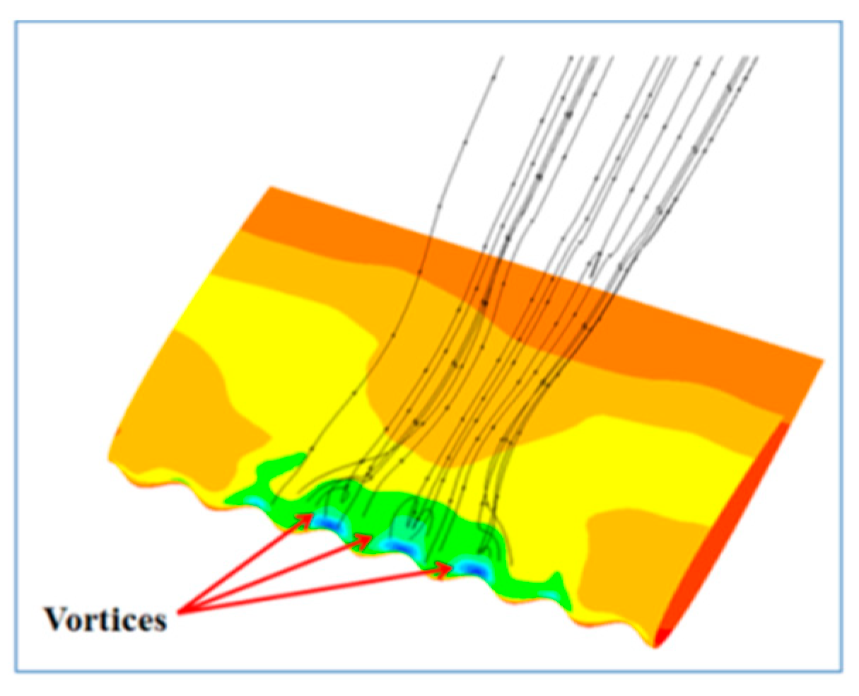
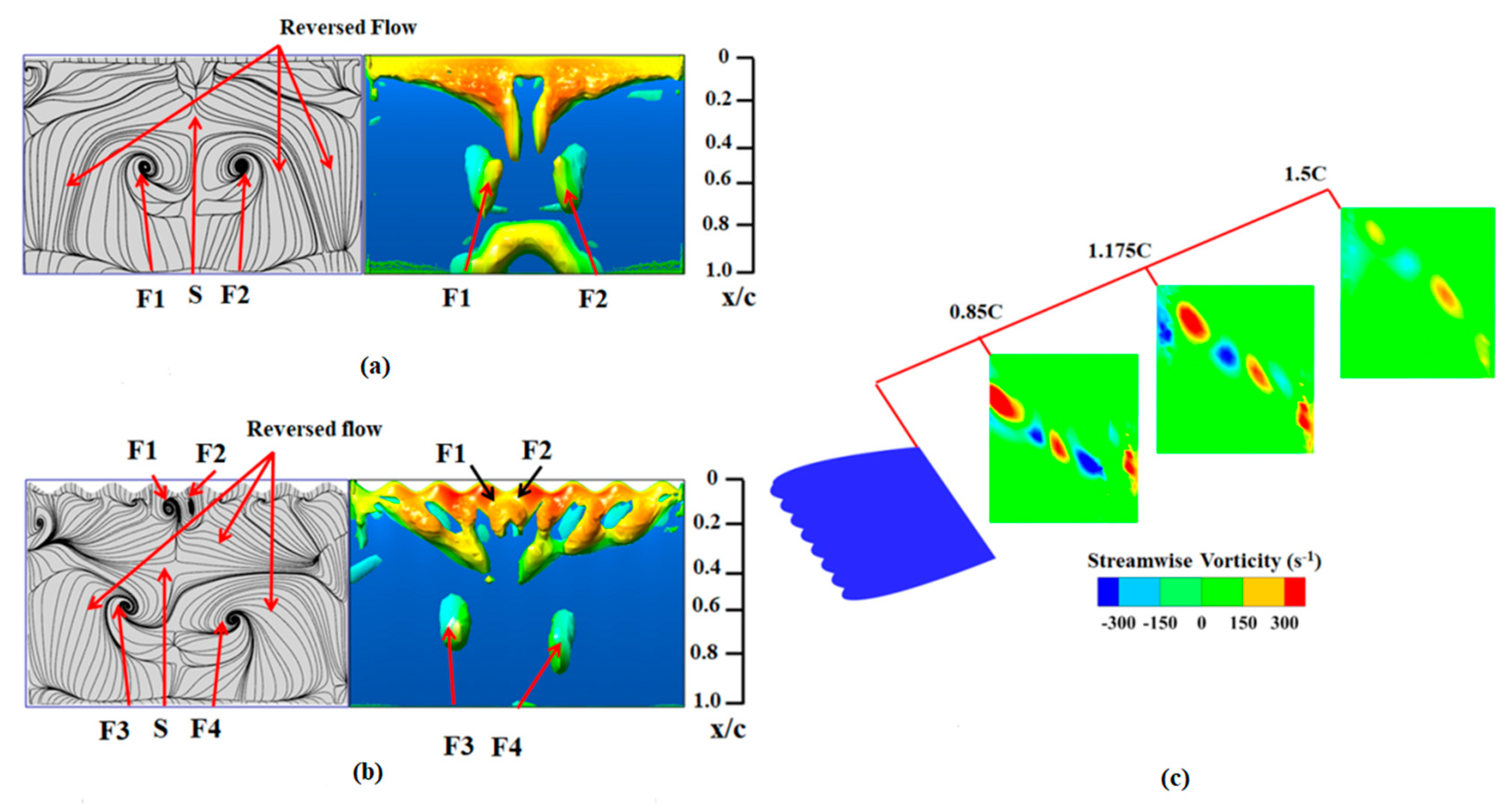
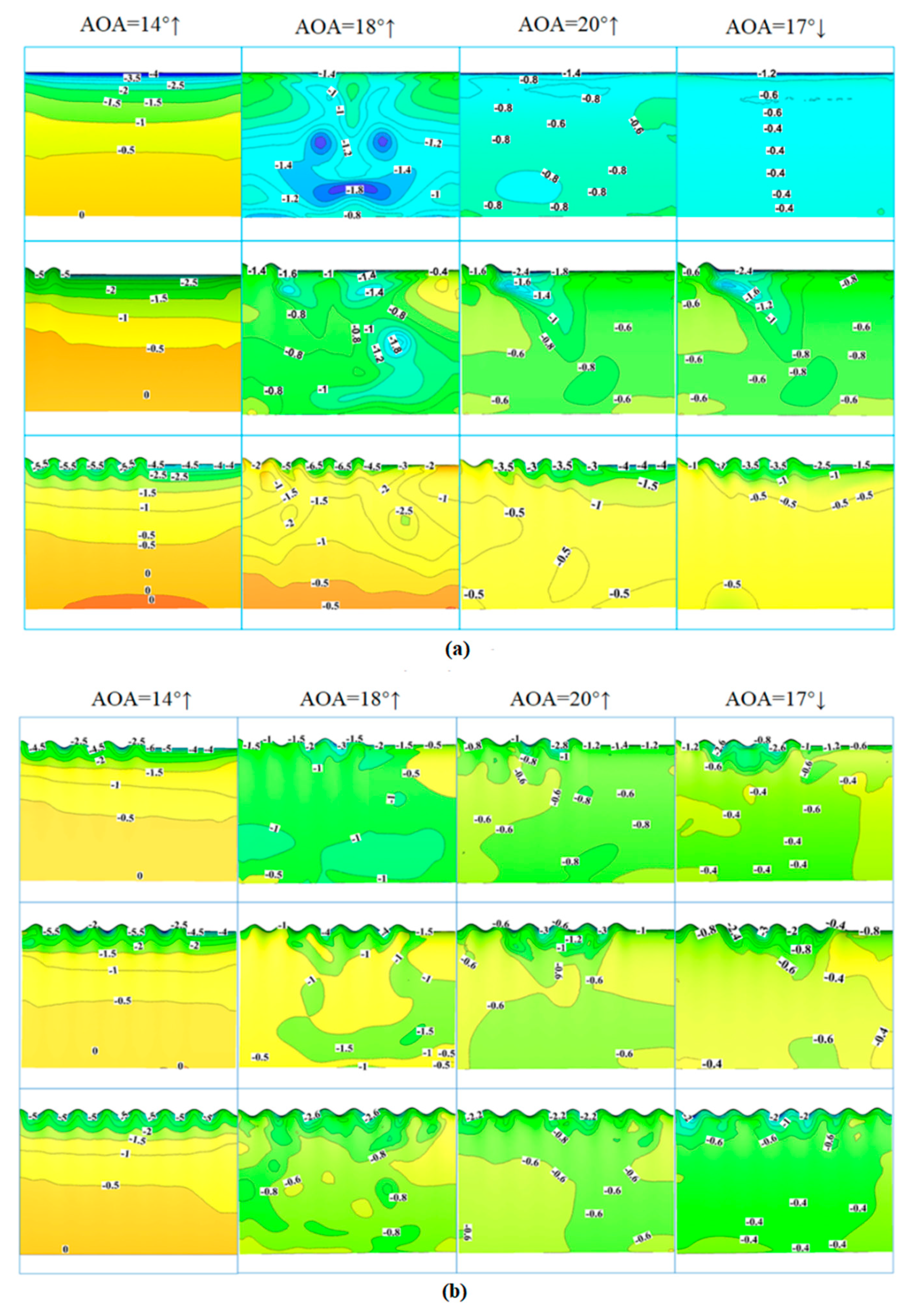
4.2. Formation of Streamwise Vorticity

The main flow mechanism of the streamwise vortex formation can be explained from two different perspectives. From the first perspective, the spanwise vorticity varies along the airfoil’s spanwise direction according to Stokes’s law due to the cyclic distribution in the spanwise direction caused by tubercles. This means that the function of the tubercles produces ripples in the spanwise vortex of the airfoil. Similarly, each tubercle can be seen as a separated finite airfoil section. Considering that this finite airfoil produces a counter-rotating tip vortex in the direction of the flow, the periodic change of the spanwise circulation leads to the generation of a counter-rotating flow vortex. The second perspective has two main mechanisms for generating flow vortices: the so-called “skew induction” and “stress induction.” The skew induction mechanism is also called the first type of Prandtl secondary flow. The stress-induced mechanism is also known as the second type of Prandtl secondary flow, which arises from the anisotropy of the turbulent flow [35].
To illustrate the formation and development mechanism of streamwise vortices from the second perspective, we took the airfoil (R = 1.0) as an example. The tilt-induced vorticity would be generated because the vorticity (such as in the boundary layer) rotates in the flow direction or rotates laterally. This quasi-inviscid phenomenon (the first kind of Prandtl secondary flow) exists in both laminar and turbulent flows (Figure 9 and Figure 10).
The flow deflection is distinguished by the changes in the curvature of the streamlines for an airfoil with a wavy leading edge. The streamlines in Figure 8 were selected to determine the structure of the significant vortex characteristics in the airflow near the airfoil surface. The sudden change of the streamline direction indicates that the vorticity reorganized near the leading edge
We further studied the flow structure of an airfoil with a wavy leading edge by examining the shear stress lines on the airfoil surface. Figure 10a,b show that a pair of rotating focal points, namely F1 and F2, appeared near the wavy leading edge of the airfoil with R = 1.0, which was reflected by the 3D streamlines. The flow field structure was consistent. A critical point appeared downstream of this area, specifically the saddle point S, which specifies the boundary of the separation bubble. There were two other focal points, namely F3 and F4, at the rear edge of saddle point S, suggesting that the airflow develops on the upper surface of the airfoil in the form of a tornado-like vortex.
In Figure 10c, the streamwise vorticity of the airfoil with R = 1.0 at an angle of attack of 18° is shown on the planes perpendicular to the streamwise direction. It can be seen that the circulation behind the trailing edge of the airfoil had a distribution in the form of a vortex pair. The vorticity at the sections 0.85 C, 1.175 C, and 1.5 C away from the trailing edge of the airfoil showed a gradual dissipation and attenuation trend.

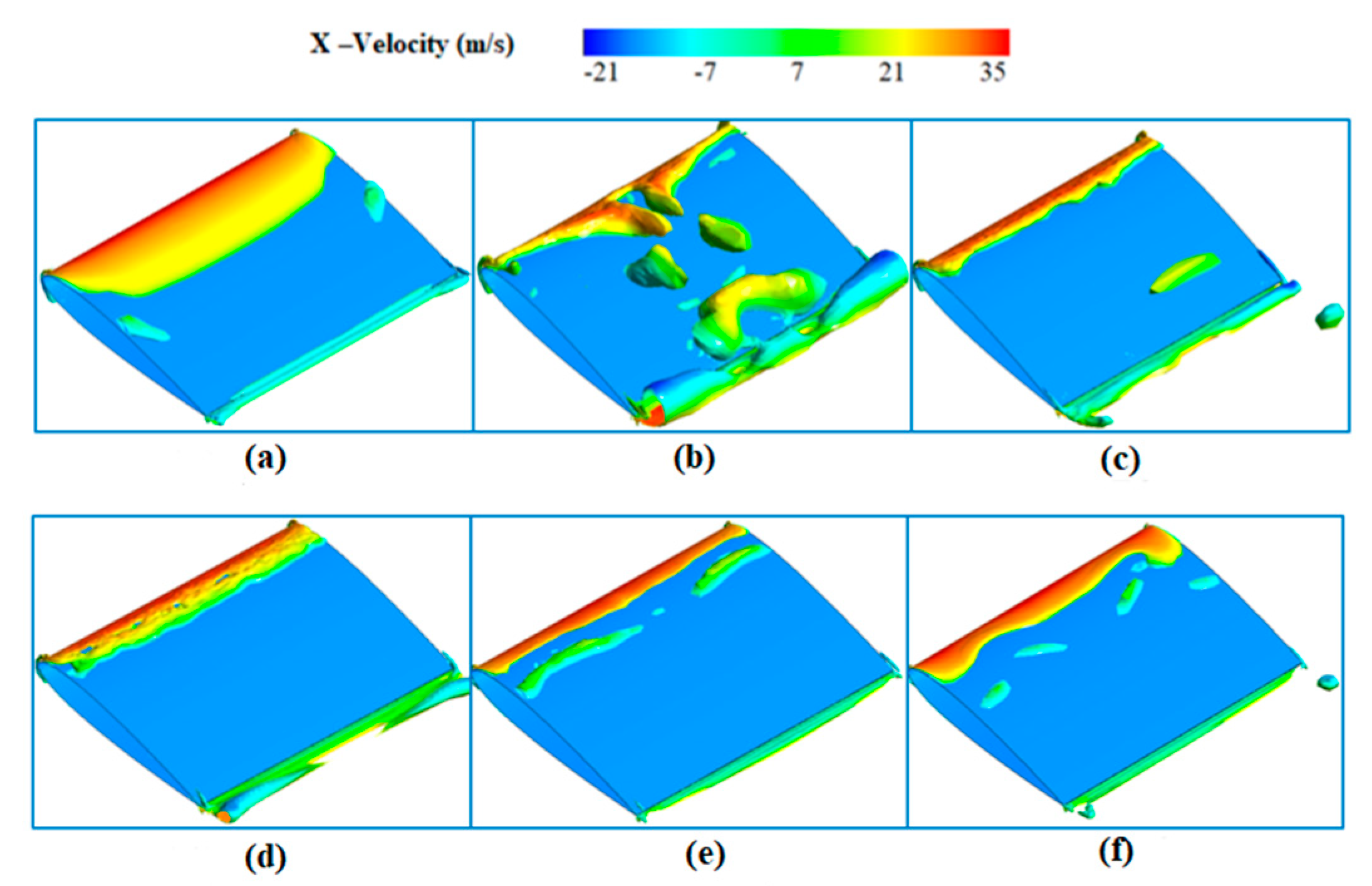
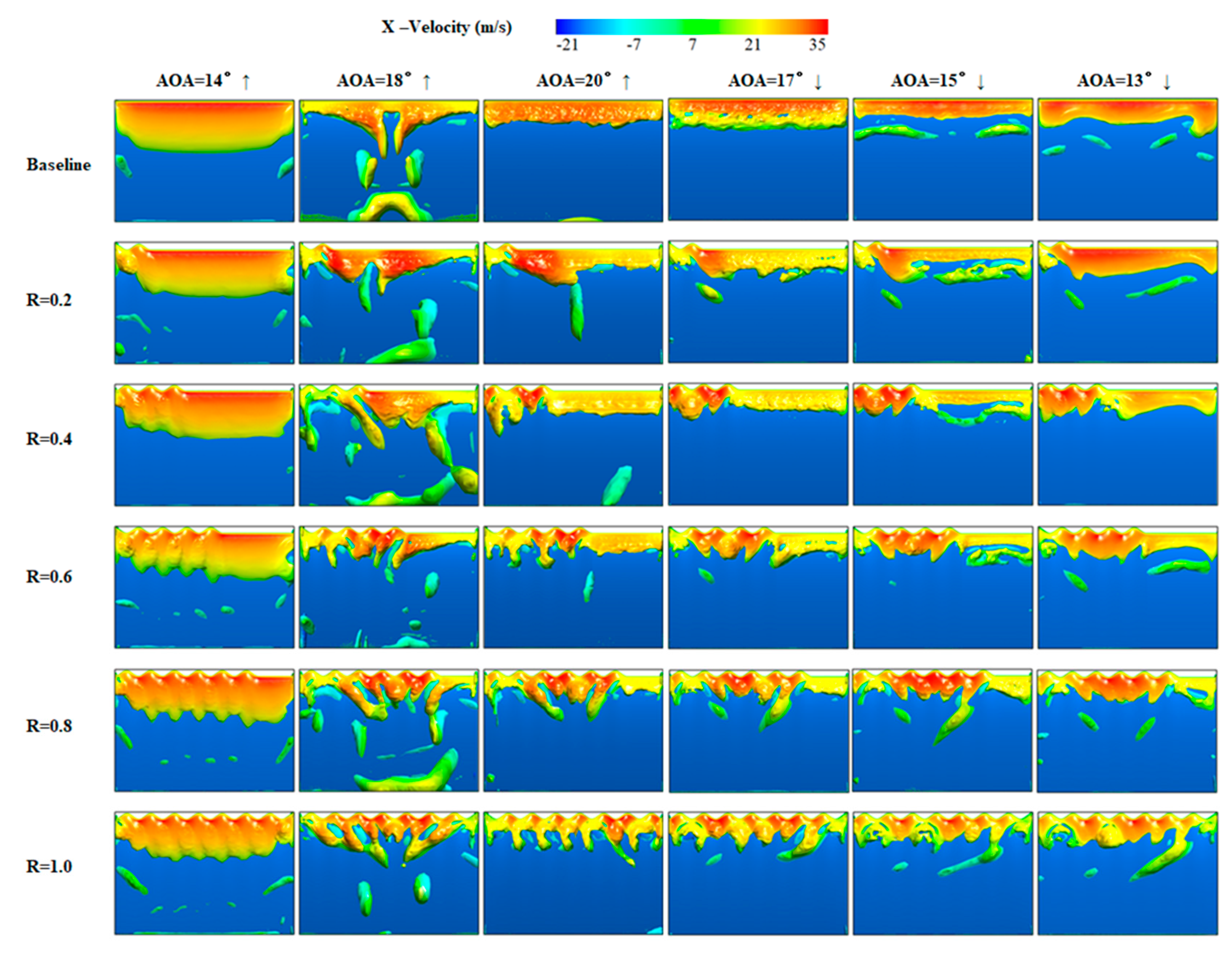
4.3. Iso-Surface of the Vorticity

The flow field structures on the different airfoils are visualized in Figure 11 to analyze the effect of wavy leading edge on the aerodynamic performance. Six different angles of attack were considered in the dynamic stall cycle. The vortex structure, in terms of the iso-surfaces of the Q-criterion, can be used to explain the flow separation on the airfoil surface. Here, we clarify the influence of different waviness ratios of the leading edge on the NACA 0015 airfoil dynamic stall characteristics.
As shown in Figure 11, the airflow on the surface of the baseline airfoil had an asymmetrical distribution at various angles of attack. When a bionic wavy leading edge was added, the vortex structure on the airfoil surface changed significantly; for instance, using an 18° angle of attack as an example, when R = 0.2 and 0.4, the symmetrical distribution of the vortex structure on the airfoil surface is broken. However, the vortex size and strength do not decrease significantly in these cases. When R = 0.6, 0.8, and 1.0, it reduces the size and strength of the airfoil surface vortex structure and suppresses the dynamic stall effect.

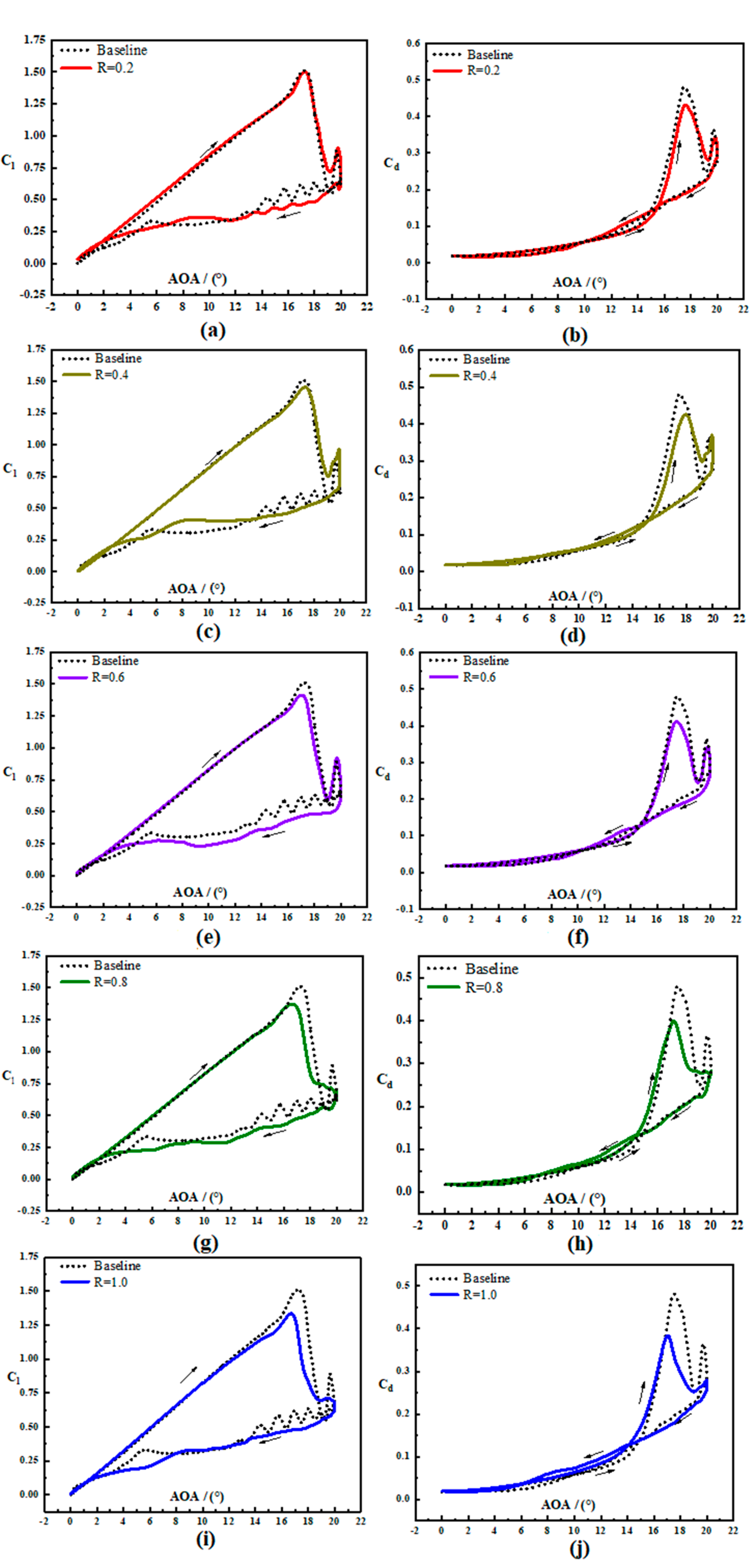
4.4. Lift and Drag Coefficients of Different Airfoils

Figure 12 shows the lift and drag characteristic curves of airfoils with different values of R, as well as the baseline airfoil in dynamic stall for a Reynolds number of 3 × 10⁵.
When R = 0.2, the peak lift coefficient of the bionic airfoil was almost the same as that of the baseline airfoil. When R = 0.4, the peak lift coefficient of the bionic airfoil decreased slightly. With increasing R, the bionic wavy leading edge gradually weakened the hysteresis effect of the airfoil lift coefficient.
When R = 0.6, 0.8, and 1.0, the bionic leading edge reduced the peak value of the lift coefficient and reduced the delay in the flow reattachment. The peak value of the drag coefficient during pitch-up was significantly reduced for all the bionic airfoils compared with the baseline airfoil, whereas the drag coefficient of each bionic airfoil was the same as that of the baseline airfoil during pitch-down.
Table 2 shows the calculated results for the maximum lift coefficient Clmax, the maximum drag coefficient Cdmax, and the ΔClmax and ΔCdmax compared with the baseline airfoil. The five bionic leading edges significantly reduced the peak drag, although with degrees of loss of lift. There were significant improvements in the drag characteristics at a small cost in the loss of lift for cases of R = 0.2 and R = 0.4.

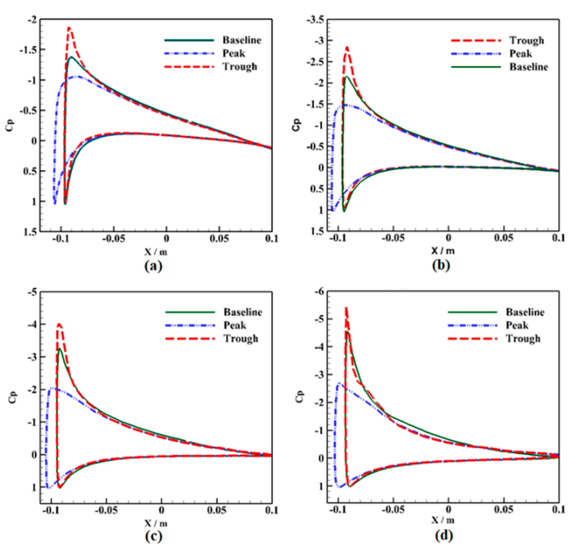
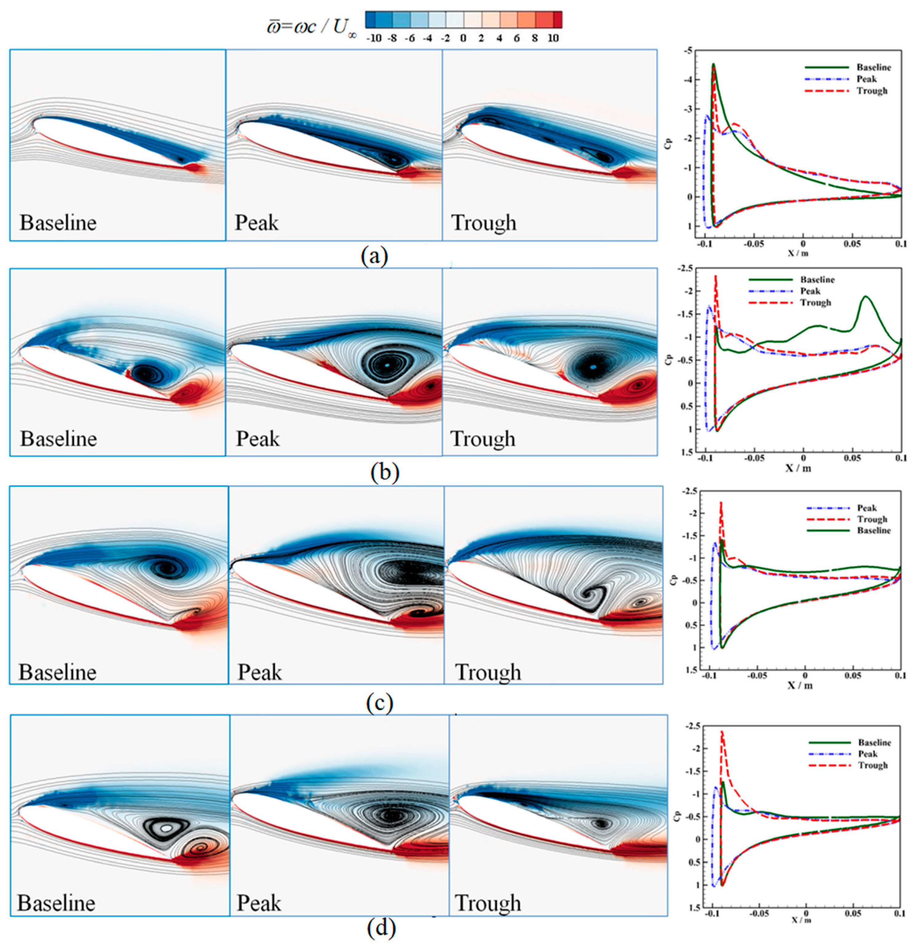
4.5. Dynamic Stall Control Mechanism of the Wavy Leading Edge

In the preceding subsections, we have qualitatively analyzed the influence of a wavy leading edge on the dynamic stall characteristics of the NACA 0015 airfoil. We now take R = 1.0 as an example to quantitatively analyze the control mechanism of dynamic stall compared with the baseline airfoil. Figure 13 shows the location of the airfoil section for this analysis.
When the angle of attack increased to 5.8°, 8.5°, and 11.2°, Cl maintained linear growth (Figure 12) and the flow adhered to the airfoil surface. A comparison of the pressure coefficients of each section is given in Figure 14, where “Baseline” represents the cross-section of the baseline airfoil, “Peak” represents the cross-section of the crest, and “Trough” represents the trough section.
With the angle of attack increased, the suction peak force on the baseline airfoil increased, while the peak suction force on the trough section increased significantly. At an angle of attack of 14.0°, Cp exceeded −5. This is because part of the airflow converges from the crest to the trough and the velocity increases. The zone of high negative pressure for the trough section increased in size and the adverse pressure gradient became stronger. Conversely, part of the airflow that was about to reach the crest was drawn by the negative pressure at the front edge of the trough, thus the acceleration effect of the flow around the front edge of the crest was weakened. As a result, the peak value of Cp on the crest section was always small.
As the angle of attack increased, the peak suction force on the airfoil increased. When the angle of attack was 16° (Figure 15a), the growth rate of Cl for the bionic airfoil changed, whereas that of the baseline airfoil was still linear. The airflow in the trough section was boosted to the average level in a shorter time. The strong reverse pressure gradient makes separating the airflow in the trough section easier and a separation vortex appeared in advance. The accompanying low-pressure effect caused a small plateau in the Cp of the trough cross-section. This further increased the lift on the airfoil in the trough section, thereby changing the Cl ratio.
Figure 15b shows the Cp curves and flow fields when the angle of attack was increased to 18°. The Cl of the baseline airfoil was close to its peak value (the lift coefficient reached its peak value at an angle of attack of 17°) and the separation vortex almost covered the upper surface. As the vortex moved downstream, the low-pressure area moved backward and the Cp peak value decreased. The airfoil with R = 1.0 stalled at this moment, the primary separation vortex began to depart from the upper surface, and the low-velocity recirculation zone covered both the trough section and the second half of the crest section.
Figure 15c shows the Cp curves and flow field for an angle of attack of 20°. Due to the gradual movement of the separation vortex away from its low-pressure zone and the vortex-induced velocity loss, the Cl of the baseline airfoil dropped sharply. Simultaneously, the counterclockwise vortex was rolled up by the separating vortex at the trailing edge, and a low-pressure zone formed, which resulting in a bow moment higher than the airfoil with R = 1.0. At this time, the trailing-edge vortex had fallen off the bionic airfoil. Even at the maximum angle of attack, a small part of the flow at the leading edge of the crest section still adhered to the airfoil surface, acting as a “wing knife” to limit the spread of the separation vortex along the spanwise direction.
When the angle of attack started to decrease, the aerodynamic coefficients of the two airfoils showed different trends. From Figure 10, it can be seen that the Cl of the baseline airfoil underwent small-amplitude oscillations, while that of the bionic airfoil with R = 1.0 changed steadily. Figure 15d shows the Cp curve and flow field when the angle of attack dropped to 17°. It can be seen from Figure 11 that the Cl of the baseline airfoil rose back to a high point because, as the secondary separation vortex moved downstream and strengthened, as depicted in Figure 15d, the lift increased. As the angle of attack decreases further, secondary separation vortex shedding causes Cl to fall.
Figure 11 and Figure 15 show that a sinusoidal bionic leading edge promotes the advanced generation of the separation vortex, but its strength decreases. Although the weaker separation vortex caused a loss in the lift peak, it significantly reduced the drag peak and suppressed the dynamic stall. Simultaneously, the bionic leading edge suppressed secondary separation vortex generation, thus the lift coefficient changed smoothly during the descent process.
Figure 16 shows the profiles of the pressure coefficient Cp of the 3D suction surfaces of the baseline and bionic airfoils at different angles of attack. When the angle of attack was 14°, regardless of the airfoil shape, the airflow was attached to all the airfoil surfaces and the pressure coefficient distribution was relatively uniform. Low Cp values were distributed near the leading edge and Cp increased along the chord direction. The distribution of Cp changed locally when a wavy leading edge was applied to the airfoil, with low and high pressures appearing in trough and peak areas, respectively. In addition, the pressure gradient behind the groove was more unfavorable than the pressure gradient after the crest because low Cp appeared in the groove. At the same time, the distance between the trailing edge and the crest was longer than the distance between the trailing edge and the groove.
For the bionic airfoil (R = 0.2), the number of waviness was the lowest and therefore this wavy leading edge had little effect on the Cp distribution, with the overall distribution of Cp being similar to that of the baseline airfoil. Even when R = 0.4, the general Cp was not significantly different from that of the baseline and the case of R = 0.2 in the distribution (Figure 16a). This is consistent with the result that the Cl and Cd for R = 0.2 and 0.4 are similar.
When R = 0.6, the effect of waviness on the Cp distribution became evident and it propagated over the whole airfoil surface, leading to the formation of a Cp wave profile. However, the average values of high and low Cp in the crest and trough regions were similar to the baseline airfoil. Therefore, the Cl and Cd values were almost the same as those of the baseline airfoil. When R increased to 0.8 and 1.0, the peak pressure coefficient on the upper surface of the bionic airfoil increased and consequently the lift coefficients for the R = 0.8 and 1.0 airfoils were different from those of the baseline airfoil. In particular, the drag coefficients of the R = 0.8 and 1.0 airfoils decrease significantly at this angle of attack.
However, when the angle of attack increased to 18°, the waviness completely changed the pressure distribution on the airfoil surface. The pressure coefficient on the baseline airfoil suction surface was symmetrically distributed but that on the bionic airfoil surface was irregularly distributed. Consistent with the conclusions obtained in Section 4, the peak pressure coefficient of the bionic airfoil appeared at the trough. Among all the bionic airfoils, the peak value of the pressure coefficient at the trough was the lowest (−6.5) for the R = 0.4 airfoil. Thus, the Cl of the bionic airfoil with R = 0.4 was the largest due to the greater pressure difference at the leading edge, as shown in Figure 12.
After the airfoil reached the maximum angle of attack, it began to move downward. It can be seen from Figure 16 that during pitching from 20° to 17°, the pressure coefficient of the baseline airfoil changed dramatically, resulting in sharp oscillations of the lift coefficient of the airfoil. Compared with the baseline airfoil, the pressure coefficient on the suction surface of all the bionic airfoils changed smoothly during pitching from 20° to 17° and thus the lift coefficient of the bionic airfoils changed smoothly at the maximum angle of attack.
In summary, when R = 0.2 and 0.4, the control effect of waviness on the dynamic stall is not apparent, especially during upward pitching from 0° to 18°, because the number of functional factors is low. For R = 0.6, with a greater number of functional factors, the inhibitory effect of waviness on the dynamic stall was moderately enhanced. When R = 0.8 and 1.0, the bionic wavy leading edge significantly improved the dynamic stall characteristics. The wavy leading edge restrains the occurrence of dynamic stall, reduces the dynamic aerodynamic hysteresis of the airfoil, and improves the stability of the dynamic aerodynamic force.

5. Conclusions

The flow around bionic airfoils with different spanwise waviness ratios under dynamic stall conditions has been studied numerically. A NACA 0015 airfoil with an aspect ratio of 1.5 was modified with a tubercle leading edge, with a wavelength of 0.2 C and amplitude of 0.025 C. Different waviness ratios including R = 0.2, 0.4, 0.6, 0.8, and 1.0 were investigated. The main conclusions from this study are as follows:
(1)
As revealed by numerical simulations, a skew-induced mechanism can explain the generation of streamwise vorticity. From another standpoint, the spanwise vorticity rippled along the span of the airfoil caused by the tubercle leading edge, which leads to the generation of streamwise vorticity.
(2)
The greater adverse pressure gradient of the trough section at the wavy leading edge promotes advanced separation. The flow on the surface of the crest weakens the effect of the separating vortex on the trough and restricts its spanwise propagation. Simultaneously, the wavy leading edge suppresses dynamic stall and prevents a delay in separation.
(3)
The application of a wavy leading edge significantly reduces the peak drag coefficient. The peak lift coefficient is also reduced but to a much smaller degree than the peak drag coefficient. For example, the peak drag coefficient of a bionic airfoil with R = 0.8 is reduced by 16.67% and the peak lift coefficient is reduced by 9.27%.
(4)
It has been demonstrated that the dynamic hysteresis effect is gradually improved as the waviness ratio increases. Thus, the area of the hysteresis loop is the smallest for the bionic airfoil with R = 1.0.

Author Contributions

L.W. conducted the study and analysis. X.L. supervised all activities. All authors have read and agreed to the published version of the manuscript.

Funding

This work was supported by the National Key R&D Program of China (number 2019YFB1504601) and National Natural Science Foundation of China (number 51676152).

Institutional Review Board Statement

Not applicable.

Informed Consent Statement

Not applicable.

Data Availability Statement

Not applicable.

Conflicts of Interest

The authors declare no conflict of interest.

Nomenclature

AOAangle of attack (°)
ARaspect ratio
awavy amplitude (m)
Cchord length of airfoil (m)
Cddrag coefficient
Cllift coefficient
Cppressure coefficient
Cl / Cdratio of the lift coefficient to the drag coefficient
C(z)local chord length of the airfoil (m)
Dω+positive part of the cross-diffusion term
ffrequency (Hz)
QQ-criteria
Rwaviness ratio
ReReynolds number
Sspan of airfoil (m)
SWspan of waviness (m)
Sijaverage velocity strain-rate tensor
UFree-flow velocity (m/s)
Y+The normalized thickness of first layer grids perpendicular to the airfoil surface
αampamplitude of oscillation (°)
αmeanmean angle of attack (°)
λwavelength (m)

References

  1. Niu, J.P.; Lei, J.M.; Lu, T.Y. Numerical research on the effect of variable droop leading-edge on oscillating NACA0012 airfoil dynamic Stall. Aerosp. Sci. Technol. 2018, 72, 476–485. [Google Scholar] [CrossRef]
  2. Karbasian, H.R.; Moshizi, S.A.; Maghrebi, M.J. Dynamic stall analysis of S809 pitching airfoil in unsteady free stream velocity. J. Mech. 2016, 32, 227–235. [Google Scholar] [CrossRef] [Green Version]
  3. Corke, T.C.; Thomas, F.O. Dynamic stall in pitching airfoils: Aerodynamic damping and compressibility effects. Annu. Rev. Fluid Mech. 2015, 47, 479–505. [Google Scholar] [CrossRef]
  4. Traub, L.W.; Miller, A.; Rediniotis, O. Effect of active and passive flow control on dynamic stall vortex formation. J. Aircr. 2004, 41, 405–408. [Google Scholar] [CrossRef]
  5. Heine, B.; Mulleneres, K. Dynamic stall control by passive disturbance generators. AIAA J. 2013, 51, 2086–2096. [Google Scholar] [CrossRef] [Green Version]
  6. Han, J.; Hui, Z.; Tian, F.; Chen, G. Review on bio-inspired flight systems and bionic aerodynamics. Chin. J. Aeronaut. 2020, 34, 170–186. [Google Scholar] [CrossRef]
  7. Wenfu, X.; Erzhen, P.; Juntao, L.; Yihong, L.; Han, Y. Flight control of a large-scale flapping-wing flying robotic bird: System development and flight experiment. Chin. J. Aeronaut 2021. [Google Scholar] [CrossRef]
  8. Huang, S.X.; Hu, Y.; Wang, Y. Research on aerodynamic performance of a novel dolphin head-shaped bionic airfoil. Energy 2021, 214, 118179. [Google Scholar] [CrossRef]
  9. Savkiv, V.; Mykhailyshyn, R.; Duchon, F.; Maruschak, P.; Prentkovskis, O. Substantiation of Bernoulli grippers parameters at non-contact transportation of objects with a displaced center of mass. In Proceedings of the Transport Means-Proceedings of the International Conference, Trakai, Lithuania, 3–5 October 2018; pp. 1370–1375. [Google Scholar]
  10. Dong, X.; Li, D.; Xiang, J.; Wang, Z. Design and experimental study of a new flapping wing rotor micro aerial vehicle. Chin. J. Aeronaut. 2020, 33, 3092–3099. [Google Scholar] [CrossRef]
  11. Chen, L.; Zhang, Y.; Chen, Z.; Xu, J.; Wu, J. Topology optimization inlightweight design of a 3D-printed flapping-wing micro aerialvehicle. Chin. J. Aeronaut. 2020, 33, 3206–3219. [Google Scholar] [CrossRef]
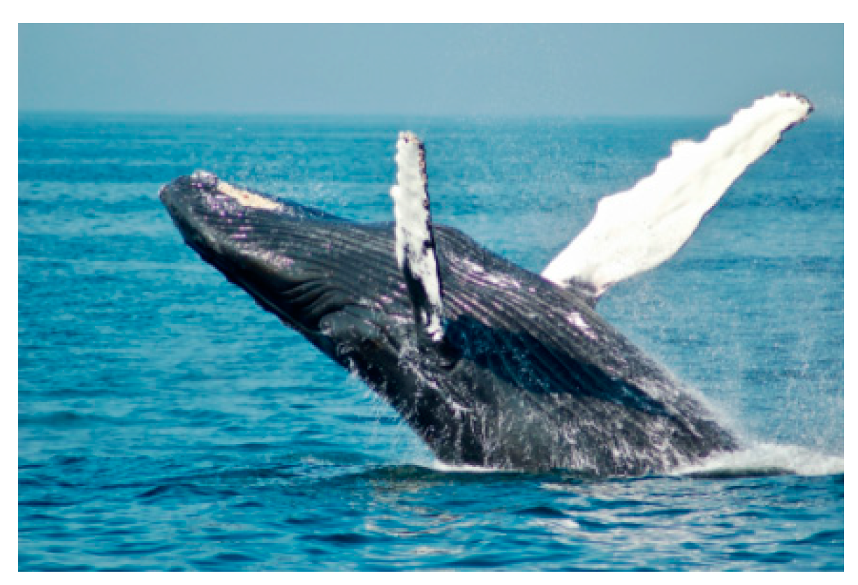
  12. Fish, F.E.; Battle, J.M. Hydrodynamic design of the humpback whale flipper. J. Morphol. 1995, 225, 51–60. [Google Scholar] [CrossRef]
  13. Miklosovic, D.S.; Murray, M.M.; Howle, L.E.; Fish, F.E. Leading-edge tubercles delay stall on humpback whale (Megaptera novaeangliae) flippers. Phys. Fluids 2004, 16, L39–L42. [Google Scholar] [CrossRef] [Green Version]
  14. Pérez-Torró, R.; Kim, J.W. A large-eddy simulation on a deep-stalled aerofoil with a wavy leading edge. J. Fluid Mech. 2017, 813, 23–52. [Google Scholar] [CrossRef] [Green Version]
  15. Serson, D.; Meneghini, J.R.; Sherwin, S.J. Direct numerical simulations of the flow around wings with spanwise waviness at a very low Reynolds number. Comput. Fluids 2017, 146, 117–124. [Google Scholar] [CrossRef] [Green Version]
  16. Hansen, K.L.; Kelso, R.M.; Dally, B.B. Performance variations of leading-edge tubercles for distinct airfoil profiles. AIAA J. 2011, 49, 185–194. [Google Scholar] [CrossRef]
  17. Yoon, H.S.; Hung, P.A.; Jung, J.H.; Kim, M.C. Effect of the wavy leading edge on hydrodynamic characteristics for flow around low aspect ratio wing. Comput. Fluids 2011, 49, 276–289. [Google Scholar] [CrossRef]
  18. Cai, C.; Liu, S.; Zuo, Z.; Maeda, T.; Kamada, Y.; Li, Q.A.; Sato, R. Experimental and theoretical investigations on the effect of a single leading-edge protuberance on airfoil performance. Phys. Fluids 2019, 31, 027103. [Google Scholar]
  19. Flores Mezarina, J.A.; Garcia Ribeiro, D.; Bravo-Mosquera, P.D.; Cerón-Muñoz, H.D. Aerodynamic effects of asymmetrical leading edge protuberances on a rectangular wing. In Proceedings of the 25th ABCM International Congress of Mechanical Engineering, Uberlândia, MG, Brazil, 20–25 October 2019. [Google Scholar]
  20. Kant, R.; Bhattacharyya, A. A bio-inspired twin-protuberance hydrofoil design. Ocean Eng. 2020, 218, 108209. [Google Scholar] [CrossRef]
  21. Fish, F.E.; Lauder, G.V. Passive and active flow control by swimming fishes and mammals. Annu. Rev. Fluid Mech. 2006, 38, 193–224. [Google Scholar] [CrossRef] [Green Version]
  22. Rohmawati, I.; Arai, H.; Nakashima, T.; Mutsuda, H.; Doi, Y. Effect of wavy leading edge on pitching rectangular wing. J. Aero Aqua Bio-Mech. 2020, 9, 1–7. [Google Scholar] [CrossRef] [Green Version]
  23. Cai, C.; Zuo, Z.G.; Liu, S.H.; Wu, Y.L.; Wang, F.B. Numerical evaluations of the effect of leading-edge protuberances on the static and dynamic stall characteristics of an airfoil. IOP Conf. Ser. Mater. Sci. Eng. 2013, 52, 052006. [Google Scholar] [CrossRef] [Green Version]
  24. Hrynuk, T.J.; Bohl, D.G. The effects of leading-edge tubercles on dynamic stall. J. Fluid Mech. 2020, 893, 1–29. [Google Scholar] [CrossRef]
  25. Aftab, S.M.A.; Razak, N.A.; Mohd Rafie, A.S. Mimicking the humpback whale: An aerodynamic perspective. Prog. Aerosp. Sci. 2016, 38, 48–69. [Google Scholar] [CrossRef]
  26. Choudhry, A.; Leknys, R.; Arjomandi, M.; Kelso, R. An insight into the dynamic stall lift characteristics. Exp. Therm. Fluid Sci. 2014, 58, 188–208. [Google Scholar] [CrossRef]
  27. Anders, J.B. Biomimetic Flow Control. CR Mec. 2000, 340, 1–2. [Google Scholar]
  28. Rival, D.; Hass, G.; Tropea, C. Recovery of energy from leading-and trailing-edge vortices in tandem-airfoil Configurations. J. Aircr. 2011, 48, 203–211. [Google Scholar] [CrossRef] [Green Version]
  29. Lee, T.; Gerontakos, P. Investigation of flow over an oscillating airfoil. J. Fluid Mech. 2004, 512, 313–341. [Google Scholar] [CrossRef]
  30. Wang, S.; Ingham, D.B.; Ma, L.; Pourkashanian, M.; Tao, Z. Turbulence modeling of deep dynamic stall at relatively low Reynolds number. J. Fluid Struct. 2012, 33, 191–209. [Google Scholar] [CrossRef]
  31. Karbasian, H.R.; Kim, K.C. Numerical investigations on flow structure and behavior of vortices in the dynamic stall of an oscillating pitching hydrofoil. Ocean Eng. 2016, 127, 200–211. [Google Scholar] [CrossRef]
  32. Kim, Y.; Xie, Z.T. Modelling the effect of freestream turbulence on dynamic stall of wind turbine blades. Comput. Fluids 2016, 129, 53–66. [Google Scholar] [CrossRef] [Green Version]
  33. Singhal, A.; Castañeda, D.; Webb, N.; Samimy, M. Control of dynamic stall over a NACA0015 airfoil using plasma actuators. AIAA J. 2018, 56, 78–89. [Google Scholar] [CrossRef]
  34. Yu, H.C.; Zheng, J.G. Numerical investigation of control of dynamic stall over a NACA0015 airfoil using dielectric barrier discharge plasma actuators. Phys. Fluids 2020, 32, 035103. [Google Scholar]
  35. Rostamzadeh, N.; Hansen, K.L.; Kelso, R.M.; Dally, B.B. The formation mechanism and impact of streamwise vortices on NACA 0021 airfoil’s performance with undulating leading edge modification. Phys. Fluids 2014, 26, 51–60. [Google Scholar] [CrossRef]
Figure 1. Humpback whale flippers with tubercles.
Applsci 11 09943 g001
Figure 2. Airfoil models. (a) Baseline; (b) R = 0.2; (c) R = 0.4; (d) R = 0.6; (e) R = 0.8; (f) R = 1.0.
Applsci 11 09943 g002
Figure 3. Computational domain and grids. (a) calculation domain; (b) local schematic of airfoil grid; (c) overall schematic of airfoil grid.
Applsci 11 09943 g003
Figure 4. Computational domain and grids. (a) grid independence verification; (b) time step independence verification.
Applsci 11 09943 g004
Figure 5. Comparison of current simulation with other results. (a) NACA0012; (b) NACA0015.
Applsci 11 09943 g005
Figure 6. Flow patterns around the baseline NACA 0015 airfoil.
Applsci 11 09943 g006
Figure 7. Vorticity with streamlines for different angles of attack. (a) 14t↑ (b) 18°↑ (c) 20°↑ (d) 17°↓ (e) 15°↓ (f) 13°↓.
Applsci 11 09943 g007
Figure 8. Iso-surfaces of vorticity (Q = 200000 s−2) with velocity. (a) 14°↑ (b) 18°↑ (c) 20°↑ (d) 17°↓ (e) 15°↓ (f) 13°↓.
Applsci 11 09943 g008
Figure 9. Three-dimensional streamlines of an airfoil (R = 1.0).
Applsci 11 09943 g009
Figure 10. Contours of streamwise vorticity with shear stress lines. (a) Shear stress lines for baseline at 18°↑; (b) Shear stress lines for R = 1.0 at 18°↑; (c) Contours of streamwise vorticity.
Applsci 11 09943 g010
Figure 11. Iso-surfaces of vorticity (Q = 200,000 s−2) with velocity for different airfoils.
Applsci 11 09943 g011
Figure 12. Lift coefficients for different airfoils. (a) Cl for R = 0.2; (b) Cd for R = 0.2; (c) Cl for R = 0.4; (d) Cd for R = 0.4; (e) Cl for R = 0.6; (f) Cd for R = 0.6; (g) Cl for R = 0.8; (h) Cd for R = 0.8; (i) Cl for R = 1.0; (j) Cd for R = 1.0.
Applsci 11 09943 g012
Figure 13. Location of the airfoil section.
Applsci 11 09943 g013
Figure 14. Comparison of pressure coefficients for different angles of attack. (a) 5.8°↑; (b) 8.5°↑; (c) 11.2°↑; (d) 14.0°↑.
Applsci 11 09943 g014
Figure 15. Flow fields and pressure coefficients of different sections at different angles of attack. (a) 14°↑ (b) 18°↑ (c) 20°↑ (d) 17°↓.
Applsci 11 09943 g015
Figure 16. Pressure coefficients for different airfoils. (a) Baseline, R = 0.2, R = 0.4; (b) R = 0.6, R = 0.8, R = 1.0.
Applsci 11 09943 g016
Table 1. Parameters for the computational case.
ParametersValuesValues
AirfoilNACA0015NACA0012
Reynolds number (Re)3.0 × 1051.35 × 105
Amplitude of oscillation (αamp)10°15°
Oscillation frequency (f)1.75071.162
Mean angle of attack (αmean)10°10°
Free-flow velocity (U)22 m/s19.72 m/s
Chord length of airfoil (C)0.2 m0.1 m
Table 2. Summary of results for different airfoils.
AirfoilClmaxCdmaxΔClmaxΔCdmax
Baseline1.510.48
R = 0.21.500.43−0.67%−10.42%
R = 0.41.490.42−1.32%−12.5%
R = 0.61.410.41−6.62%−14.58%
R = 0.81.370.40−9.27%−16.67%
R = 1.01.340.39−11.26%−18.75%
Publisher’s Note: MDPI stays neutral with regard to jurisdictional claims in published maps and institutional affiliations.

