1. Introduction
Augmented reality audio (ARA) [
1] represents a well-established sound engineering foundation that typically relies on mixing the real sonic environment of a listener with an artificial sound component to produce a new complex and immersive acoustic field carrying multiple layers of information. To achieve the desired immersion, an ARA headset and binaural rendering technique [
2,
3] are employed. Due to this rather simplistic and portable two-channel realization, ARA is currently utilized in a wide range of applications, including museum tours [
4], audio games [
5,
6,
7,
8], impaired people aids [
9,
10], navigation [
11,
12], tourism [
13,
14], and even sound art [
15].
The most critical aspect of ARA is mixing the real with the virtual audio information. The goal is the smooth integration of the virtual audio component with the real acoustic world. In that context, sound spatialization is a significant perceptual parameter; the employed virtual sound source localization techniques, as well as specific psycho-acoustic phenomena (i.e., the precedence and masking effects), directly affect the degree of immersion and the capacity of the conveyed information. Moreover, the synthesis of the virtual content must ensure that the listeners do not become isolated from their real environment or lose any associated information that needs to be retained invariably after mixing.
Figure 1 illustrates the typical architecture of the ARA mixing process, as defined by [
16]. Using binaural recording, the real acoustic environment of the listener is transformed into a pseudo-acoustic one, which is further mixed with the virtual sound field derived through binaural processing. The final AR output is driven back to the listener through headphones.
Several studies already exist that focus particularly on the efficiency of ARA mixing through binaural reproduction of the real sonic environment [
3,
17,
18]. In the so-called ARA mixer, the real environment is blended with the content of a virtual world, typically under a fixed mixing gain. However, this technique ignores the dynamic nature of both sound components, rendering their dynamic integration impossible in terms of audible clarity or a target-fixed audible difference. To address this restriction, one has to continuously adjust the gain of the virtual audio engine or redefine the mixing gains dynamically. Thus, human auditory properties (such as loudness) should be considered through a strategy that applies targeted features on the ARA components according to specific, predefined rules. To that end, mathematical models that estimate the human auditory perception, for example, binaural loudness [
19,
20], should be employed.
The development of a dynamic ARA mix technique is impeded by two practical limitations: the large amount of multi-channel audio data and the real-time signal processing latency. The same restrictions also apply to the field of intelligent multi-channel audio systems [
21,
22]. To address these challenges, this study aims to develop an ARA mix model using rigorous criteria based on psycho-acoustic parameters that model loudness sensation. As a result, ARA technology is “reintroduced” from a perceptual perspective.
This paper is organized as follows:
Section 2 provides a brief but focused theoretical overview of ARA mixing.
Section 3 examines the proposed model’s technical design and implementation. In
Section 4, the methodology of the conducted subjective evaluation is presented. The results obtained are described in
Section 5, and further discussed in
Section 6. Finally,
Section 7 concludes the work and provides some considerations for future work.
2. Theoretical Background
In ARA, both the real and virtual sound components are equally crucial for achieving an immersive experience [
23]. In practice, this notion of “equality” is somewhat vague, since it can be interpreted in two ways: the virtual environment energy can either serve as the reference point of the mix adaptation or be adjusted to match a corresponding real environment energy reference. In this research, the second alternative is followed—the ARA mix adaptation is determined by the virtual component adaptation relative to the real environment reference energy and consequently to the natural hearing level of the real acoustic world. This decision was taken due to the fact that the real environment should not be altered in a mix; hence, only the ARA virtual tracks should be adjusted.
Regarding perception and sound signal energy, it is well-known that loudness describes how loud the acoustic environment is perceived. In that context, loudness sensation is a subjective attribute of sound that expresses acoustic energy in terms of auditory perception. In the literature, one can find a variety of mathematical models for loudness analytic descriptions [
24,
25,
26]. In addition, a set of mapping contours are already derived to describe the loudness of different sound fields [
27,
28,
29], while a variety of loudness models, such as binaural loudness [
19,
20], aim to predict the loudness of binaural hearing.
ARA mainly employs binaural rendering for sound reproduction since it provides a number of implementation advantages: the use of headphones prevents cross–talk between ears, whereas binaural spatialization achieves better localization perception of the virtual sound source images and improves the spatial separation in the case of multiple active sources [
30]. Hence, following this legacy employment trend, any attempt to provide a dynamic ARA-mixing mechanism should consider binaural loudness.
In the past years, a number of models that predict binaural loudness have been proposed [
20,
31]. They allow for the quantification of human auditory perception, but their use is impeded by several factors. For example, excessive processing power makes real-time loudness estimation problematic [
32]. Tuomi [
33] implements a model based on C-code that could be used to calculate the specific loudness of 8192 sample windows in 20 milliseconds. Ward’s work [
32] also emphasizes the efficiency of real-time implementations. Recent research efforts have employed deep neural network architectures [
34], where it is noted that training with pure tones and noise ensured that the effects of level, frequency, and spectral loudness summation are adequately represented. The use of pure tones was also investigated by the authors in a previous work [
35], in which a preliminary binaural loudness estimation methodology for the dynamic ARA mix model was introduced.
Figure 2 illustrates the proposed dynamic ARA mix process using a real-time prototype feature extraction technique based on the binaural loudness model of Glasberg and Moore [
19]. The core process is the binaural loudness (
BL) adaptation algorithm. This aims to control the actual levels of the virtual sound sources based on the desired binaural loudness level difference between the real and virtual sounds. Towards this aim, the feature extraction block exports the auditory excitation bands’ matrix through fast Fourier transformation (FFT) analysis. This analysis derives the actual relative level differences and maps them through a precalculated
BL matrix to a specific mixing gain of the virtual signal. Signal calibration of the real and virtual audio sources is crucial for the
BL adaptation algorithm in the perceptual domain. As a consequence, all input signals are initially calibrated to the desired energy level (dB SPL) according to the system specifications prior to the feature extraction and
BL adaptation procedure.
The selection of the headphones is a critical factor for ARA. A comparison between different headphone sets [
23] argues for choosing open headphones over closed-end ones, because the former do not obstruct the external sound. Instead, they allow it to be perceived naturally, which is quite helpful for the immersive reproduction of the real environment. However, open headphones do not block the ear canal entrance, which is essential for the propagation of the virtual component’s spatial characteristics through head related transfer functions (HRTFs), since these are commonly not measured at the eardrum, but instead at the entrance of a blocked ear canal [
36]. Another factor supporting the use of closed headphones is that much of the advantage of headphone equalization can be obtained by using a generic filter that takes into account only the resonance of the headphones themselves and not the individual anthropometry [
37]. Last, an ARA mixer requires a low latency headphone reproduction system with additional equalization to compensate for the attenuation between the modified ear canal resonances caused by headphones [
3]. Considering the above factors, the dynamic ARA-mixing strategy proposed here uses in-ear headphones that apply a sequence of filters on ear canal resonances, on the occlusion effect, and on the pressure chamber principle. Consequently, headphone audio data is measured and its energy is taken into account by the
BL adaptation algorithm before shaping the final audio result.
3. Technical Overview
The primary functionality of the proposed dynamic ARA mixing process is based on a real-time auditory model that defines the binaural loudness of the virtual sources in the final ARA signal. This definition is performed using a target loudness difference value with the reference being the measured loudness of the real acoustic world.
Figure 3 illustrates the overall architecture of the dynamic ARA mix model. The real and virtual environment signals are both fed as inputs. The real component is pre-filtered to reduce the closed-ear audio effects due to the use of headphones, and then the input signals are set for calibration. The calibration procedure is applied to the input signals to assign each with a desired level of dB SPL. An FFT analysis algorithm analyzes each calibrated signal and an operation sorts the analyzing signal into specific frequency bands, thus, creating the excitation pattern of input signals. The energy information of the signal constitutes the first part of the
BL adaptation input. The second input consists of the results of the analysis performed by the filter bank on the virtual source. The analysis filter bank deconstructs the virtual signal in the same frequency bands that have been determined by the
BL model. The
BL adaptation block defines the coefficients, as well as combines the binaural loudness model, the virtual source, and the real environment. A synthesis filter bank constructs the
BL adapted virtual signal. As a result, the signal is exported for spatialization.
The whole procedure is described in seven subsections: the first is the construction of the BL conversion matrix, the second is the signal calibration of the real and the virtual audio components, the third is the auditory excitation calculations, the fourth is the filter bank construction, the fifth is the BL prediction algorithm, the sixth is the BL adaptation algorithm, and the seventh contains the implementation overview.
3.1. BL Conversion Matrix
The
BL conversion matrix in
Figure 4 represents the conversion of the sound energy from dB SPL to
BL (Phons) for specific frequencies. The rules that govern the proposed model are concentrated in this matrix. The frequency as the reference point of
BL and dB SPL calculations reflects the central frequencies of an octave band analysis. The frequencies of interest are (a) 250 Hz, (b) 500 Hz, (c) 1000 Hz, (d) 2000 Hz, (e) 4000 Hz, (f) 8000 Hz, (g) 16,000 Hz. For each frequency, a sequence of calibrated pure tones of five seconds with 1 dB difference from 30 dB SPL to 94 dB SPL is constructed. The Glasberg and Moore model [
19] with the implementation of the Genesis toolbox [
38] analyzes each audio sample.
3.2. Calibration Procedure
Of utmost importance in the ARA mix measurements, especially for the feature extraction block, is the calibration of the signal inputs. This procedure converts the signals from the normalized amplitude levels of the signal processing programming environment (Matlab-Simulink [
39]), which range from −1 to 1, and displays them as the desired dB values. Similarly, the calibration procedure in the
BL ARA mix calibrates the signals of the real environment and the signal of the virtual source. The same calibration procedure in dB SPL values is also applied on the pure tones, which were used for
BL transform matrix construction. Tests during the simulation have shown that adjusting the calibration term to an 82 dB reference to have a value slightly greater than that helps the function of the
BL ARA mix model.
3.3. Auditory Excitation Calculation
The auditory excitation energy calculations of the model are accomplished in four stages. This procedure measures the energy of each input signal under specific limitations. The window size of real-time processing defines the principal limitation of this procedure and regulates the number of frequency bands. Moreover, a dynamic sorting algorithm has a decisive role in the BL adaptation block for the smooth operation of the ARA mix and hence for the desired audible result.
In the first stage, the calibrated input signals are transformed into the frequency domain to obtain the energy of the predetermined real-time 1024 simulation sample window. The FFT for spectral analysis was chosen as an effective function for real-time implementation in the frequency-domain. In the second stage, the input signals in the discrete frequency domain are divided into frequency bands that are of non-equivalent one octave band levels. The analysis according to FFT bins allows for the following 7-band separation with central frequencies of 0.25 kHz, 0.5 kHz, 1 kHz, 2 kHz, 4 kHz, 8 kHz, 16 kHz. The third stage of the energy calculation pipeline is to compute the average energy of each frequency band, which is subsequently represented as dB SPL intensity. The fourth stage consists of a dynamic sorting algorithm, which defines the final energy of each band in the time domain. This sorting algorithm allows the energy of each band to take specific values within specific thresholds, and thus helps to control the final energy values and to avoid high instant spectrum fluctuations, which could affect the function of the
BL adaptation algorithm. The dynamic sorting algorithm makes a real-time check according to four defined thresholds that were tuned during the real-time testing of the model
Figure 5. More specifically, two low thresholds of a three dB increase and decrease and two high thresholds of a 28 dB increase and decrease were set to control the occasion of high fluctuations of energy and validate the return of energy variables in the next lower or higher position, respectively.
3.4. Filter Bank Implementation
During the signal processing of the virtual input, the calculated coefficients are integrated after the
BL adaptation algorithm. Therefore, a filter bank was realized that consists of seven non-uniform FIR filters [
40], whose central frequencies match the central frequencies of the
BL conversion matrix (see
Figure 6). The seven filters were one lowpass, one highpass, and five bandpass filters. The Parks-McClellan [
41] algorithm was used to implement the best possible FIR filter to provide the optimal frequency response according to
Figure 6, and with the smallest number of coefficients.
Table 1 presents the central frequency and filter band of each filter according to 50% filter overlapping. Computational constraints impose the use of a 7-band filter bank during the real-time simulation of the model.
Table 1 presents the central frequency of each filter. The overlap of the filters is 50%. Computational constraints impose the use of a 7-band filter bank during the real-time simulation of the model.
Realizing the appropriate filter types is crucial for the analysis and reconstruction of different types of sound sources. Currently, the model includes a simple implementation of a filter bank for the artificial sounds employed in the testing session. In a future development of the model, a dynamic system of filter banks could be used, which will depend on the type of virtual source (speech, music, and artificial sounds).
3.5. BL Prediction Algorithm
The auditory excitation matrix of each input signal is inserted in the
BL prediction algorithm. To predict the
BL from the auditory excitation matrix, the following methodology was implemented. The excitation matrix of the signal of the pseudo-acoustic environment and the signal of the virtual environment was introduced in the
BL calculation algorithm (
Figure 7). Then the excitation values are converted to
BL values according to the acoustic energy conversion table. The algorithm searches for the nearest
BL value corresponding to the specific auditory excitation energy value for each predefined frequency band. The results for each predefined zone compose the
BL matrix for each environment. The
BL matrices represent the perceptual characteristics according to which the adapted mix works.
3.6. BL Adaptation Algorithm
The adaptation algorithm implements the integration of auditory perceptual features into the ARA mix (see
Figure 8). Its input consists of the calculated
BL matrices for the input signals of the real environment and the virtual one.
The task of the BL adaptation algorithm is to estimate the BL difference between the same bands of the virtual and real components, as well as to calculate and apply the correlation coefficient of the BL difference of each band to the BL of all bands. The following functions present the methodology of the BL adaptation algorithm.
Estimation of the
BL difference in each n frequency bands. The algorithm estimates the difference between the same band of the real and virtual components.
Estimation of the
BL environment matrix average loudness of
n frequency bands of the virtual signal.
Estimation of the correlation coefficient of the
BL band according to the average
n BL bands of the virtual signal. This function estimates the correlation coefficient of the
BL difference of each band to the
BL average energy of all frequency bands, which the model applies to each virtual band.
The estimation of the
BL constant increases or decreases compared to the initial
BL of the specific frequency band of the virtual signal. This procedure smooths the difference of each virtual band to the real one with respect to the average
BL of all n bands. Thus, any distortions are eliminated, and the changes that follow the original virtual spectrum form without any loss in originality.
Finally, the
BL constant of each band is integrated. The final coefficient for each virtual band is sent to be applied by the algorithm in the corresponding filter bank’s signal.
The integration of only the difference between the real and virtual energy bands in terms of BL evokes unpredictable changes in the virtual environment. To define the bounds of this difference, the correlation coefficient was inserted. Tests during the implementation process have showed that the correlation coefficient improves the performance of the BL adaptation algorithm and produces a smooth audible result without distortions.
3.7. Implementation Overview
Implementing the real-time function of the adaptive ARA mix model (see
Figure 9) was a challenging procedure due to the following restrictions: (a) the low-latency of the model, and (b) the sound quality of the synthesized virtual sound source. The model was developed in Simulink, the programming environment of Matlab for simulations. The window size was set at 1024 samples and the sample rate at 48 kHz. The system was single-rate. The window size was restrictive for the FFT analysis and for the sampling time of the model. Tests have shown that the window size of 1024 samples can support the adaptive ARA mix model of a seven band analysis. Furthermore, the window size of 1024 samples affects the smoothness of mixed signals, because of the dynamic level changes in frequency bands. After empirical tests, the use of a filterbank with 50% overlapping between filters was chosen, as referred to in
Section 3.4. Besides the programming environment, a TASCAM US-16x8 soundcard was used as an audio interface. Additionally, a mini mixer (Behringer XENYX502) was used for routing, and an i7 860 with 8gb ram computer for processing.
For the binaural recording of the real environment and the ear canal filter implementation, the evaluation board of analog devices—ADAU1761
Figure 10 and the in-ear headset of Philips SHN2500
Figure 11 with the noise cancellation system disabled were used.
In addition, a module was added to the GUI to facilitate the control of the
BL difference between the virtual and real component. The purpose of this was the investigation of different
BL mix loudness modes, i.e., of the effect of different mix levels on the audience. In the final implementation there are three such
BL mix loudness modes: one mode of zero difference between real to virtual acoustic environment, one of three and one of six phons difference (low
BL mix, medium
BL mix, high
BL mix). Through the GUI that controls the model and the demo sessions, the virtual source and real environment recordings were selected to be propagated through the speakers,
Figure 12. There is also the option of a 3-scale
BL mix mode (low, mid, high). Finally, the option of automatic or manual spatialization of the virtual source is provided, as well as some advanced controls for extra adjustments of the
BL mix. Essentially, the user does not need any of these controls in an ARA scenario, except for the knob of the audio augmentation level to personalize the mix.
4. Evaluation Procedure
The evaluation procedure consisted of two parts: (a) some benchmarks of the
BL ARA mix model that present the ARA mix adaptation of the model in different situations, and (b) the sound evaluation using the MUSHRA (multi stimuli hidden reference and anchor) tests [
42] of the ARA mix within a hypothesis testing framework.
4.1. Benchmark Results
In general, the testing of the model’s performance was conducted using the same BL model, which was used for the BL matrix construction. The BL analysis exports the benchmark of all inputs and outputs of the real and virtual components. The results show the model’s prediction of the binaural loudness and the adaptive mix’s response.
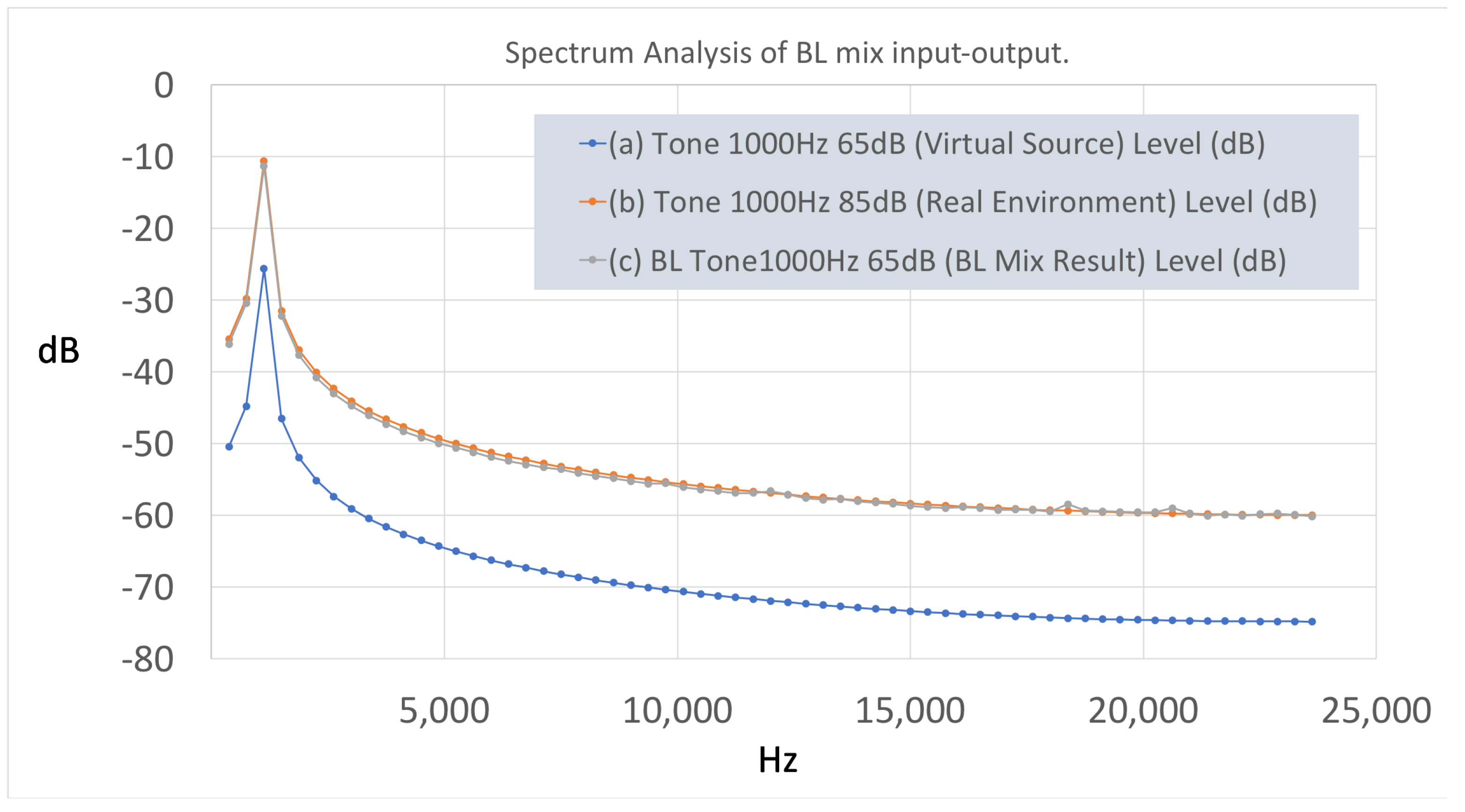
Figure 13, shows the spectrum analysis of the pure tone of 1 kHz at different dB SPL levels. The tone of 65 dB SPL (see
Figure 13a), represents the virtual input of the system, and the tone of 85 dB SPL (see
Figure 13b), the real component.
Figure 13c presents the virtual output of the
BL adaptation according to the real component. The form of the spectrum does not have any difference except for an increase in its energy. In terms of spectrum analysis, data from
Table 2 show the increase of
BL in the virtual output according to a real input tone of 1 kHz at 85 dB. The model seems to work well in this simple occasion of the ARA scenario.
Figure 14 shows the case of an ARA scenario of an artificial sound integrated in the real environment of a car traffic soundscape. According to the results in
Figure 14c, the
BL ARA mix model seems to preserve the originality of the virtual component (
Figure 14a). After the adaptive ARA mix model, the form of the Test-1 virtual input and output seems to have characteristics with energy modifications, which are relative to the changes in coloration of the
BL virtual output according to the real environment. Besides the frequency spectrum analysis, the loudness of each sample was measured for its loudness with the
BL model [
38].
Table 3 provides the results of the
BL analysis of the virtual input and the real environment, and the result of the
BL ARA mix model. The results show a decrease in loudness of the virtual output compared to the virtual input, whereas the final loudness is close to the real input of the traffic. This modification has not destroyed the final form of the spectrum, and so the virtual output does not include audible distortions.
The last ARA mix pair examined was the Test-1 virtual sound according to the previous test mixed with the real environment consisting of forest sounds. The results of the spectrum analysis are shown in
Figure 15. The real environment of the forest appears to have increased energy in a broad frequency spectrum. The model seems to have changed the spectrum of the virtual component according to the energy of missing frequencies. This analysis does not show the loudness of the audio result in comparison to the real and virtual environment.
Table 4, shows the estimation of the
BL of ARA mix components. According to this, it seems that the model has adapted the virtual component (77.17 Phons) to the real environment input (72.46 Phons), resulting in the final adapted virtual output at 72.85 Phons. The adapted virtual environment has
BL very close to the real environment, thus integrating acoustically the latter’s coloration characteristics while maintaining the originality of the virtual sources.
Overall, the results derived from the spectrum analysis of the ARA mix components and the calculation of each one’s BL indicate that the BL ARA mix model integrates the virtual environment in the real environment in a smooth way. Nevertheless, more research needs to be done to address a wide variety of different types of sound in order for the BL ARA mix model to be improved and optimized. In that process, a more sophisticated system of an adaptive filter bank model dealing with different virtual source types can be developed.
In the experiment discussed in this paper, a factor was added to control the adaptive mix level. Technically, this factor inserts a constant of three phons or six phons virtual–to–real component difference into the BL adaptation algorithm besides the normal function of zero phons.
Table 5 presents the
BL calculation of the addition of the variable of the
BL mix mode. The virtual sound was the Test-1 (same sound with benchmark tests), and the real environment was the sample of the car traffic.
According to
Table 5, the mix mode affect the
BL of the
BL virtual output as follows: the
BL adaptation algorithm increases the
BL virtual output according to the mix mode, but this increase is not strictly proportional to the characteristics of each mode, i.e., the output amount is not doubled to match the double-level difference of zero to three phons and six phons, respectively. These results are due to the energy calculation algorithm and the application of the correlation coefficient in the
BL adaptation algorithm, which act sequentially in order to maintain the originality of the virtual source.
4.2. Subjective Evaluation
The subjective evaluation of the
BL ARA mix model was a challenging procedure consisting of a MUSHRA test (see
Appendix A Figure A4). It was set up in the laboratory with stereo loudspeakers propagating the real environment, and the subjects answering an electronic questionnaire. A user-friendly graphical user interface (GUI) facilitated the evaluation system’s usability (see
Appendix A Figure A1). The system produced test samples and adapted the virtual component into the real source in real-time.
The evaluation test consisted of the following three parts: (a) demographics and technographics, (b) discrimination test, and (c) MUSHRA test. The subjects participated in the tests without any training. A number of 78 participants were recruited through email and other online communication channels.
Prior to the testing procedure, all subjects signed a statement of consent. The first part of the test required the participants to fill in their personal demographic and technographic information (see
Appendix A Figure A2). The questionnaires were submitted anonymously. In the second part, a discrimination test aimed to separate the subjects (see
Appendix A Figure A3) according to their experience in sound perception. This discrimination test included: (a) a loudness comparison test of two different tones, (b) a perception test, in which one of two tones heard separately was to be identified as a partial of a subsequent complex tone, and (c) a spatial perception test, in which subjects had to find the position of a virtual sound in a hypothetical virtual sonic environment. The number of the correct responses assigned the subject to one of the following categories: “Naive”, “Beginners”, “Experienced”, or “Experts”.
The third part of the evaluation was the MUSHRA test,
Appendix A Figure A4. The MUSHRA test consisted of five alternatives: the
BL ARA mix and four other mixes. More specifically, it was comprised of: (a) the original virtual source, (b) the
BL adapted ARA mix virtual source, (c) the original virtual source with 3.5 kHz bandwidth, (d) the original virtual source with 7 kHz bandwidth, and (e) the original virtual source with 10 kHz bandwidth. The MUSHRA’s sound content is composed of industrial sounds, which represent the real environment, and an artificial sound, (called Test-2), in looping playback mode, which represents the virtual component. At first, the subjects needed to push a button to let the system propagate a complete ARA mix in real-time. To evaluate the outcome, the participants used a Likert-type scale with the following rating options: 1. Bad, 2. Poor, 3. Fair, 4. Good, 5. Excellent.
This methodology produces qualitative data, which describe subjects’ subjective experience, to be collected in a quantitative form. The BL mix mode (low mix mode, mid mix mode, or high mix mode) was chosen randomly before the start of the test.
5. Results
The results were collected automatically by the simulation environment and imported for statistic analysis in a spreadsheet software. Firstly, they were analyzed without any classification and consequently with classification in specific categories. These categories were constructed according to the discrimination test and the BL mix mode. More specifically, the ones specified by the discrimination test were: (a) beginners, (b) experienced, and (c) experts, and the ones formulated according to the BL mix mode were; (a) low mix mode, (b) mid mix mode, and (c) high mix mode.
The number of participants in each group was:
Total number of participants: 78;
Naive: 3, beginners: 27, experienced: 26, experts: 22;
Low BL mix: 26, mid BL mix: 26, low BL mix: 26.
In each category, a
T-test between the mean of the
BL virtual mix and the means of other groups determines if there is a significant difference between the respective two groups.
Table 6,
Table 7 and
Table 8 present the
T-test results.
Generally, in
Table 6, the
BL mix results seem to outperform the alternative ARA mixes. Furthermore, the box plots of each analyzed group indicate that the
BL ARA mix has a different distribution, approximately 3 to 5, than the other mixes.
Besides the distribution analysis (see
Figure 16), the
T-test method was applied on pairs of the
BL virtual source and each of its other alternatives. The hypothesis of the
T-test examines the relation of the
BL adaptation to the unfiltered virtual signal through a comparison in the MUSHRA test. The subjects compared each ARA mix result to evaluate the quality of each mix.
Testing hypothesis:
Null hypothesis: the BL adaptation does not affect the ARA mix;
Alternative hypothesis: the BL adaptation improves the ARA mix;
Question: evaluate the mix adaptation of the virtual source in the real environment.
According to the
T-test results, the null hypothesis is rejected (
p < 0.05), except for the case of the six phons mix (
BL high mix mode), which seems to have caused confusion (
Table 7). Moreover, in the beginner and experienced groups, the
T-tests indicate that the virtual source with lower bandwidth 7 kHz, and 10 kHz, respectively, does not make a significant difference in the ARA mix (
Table 8).
6. Discussion
This study aims to identify the effect of a novel adaptive BL ARA mix to auditory perception in ARA environments. The implementation of the adaptive BL ARA mix model addressed auditory perception in an adaptive ARA mix with promising results as exhibited by the majority of the test results regarding the adaptive mix averages that have been found significant in the T-test analysis. More specifically, the results regarding the addition of the mix intensity modes have shown that the increase in the intensity mix constant does not result in a better adaptive mix for the subjects’ auditory perception. Instead, there is a limit in the BL mix constant at the three phons constant, since the six phons constant has a lower average compared to the zero and three phons cases.
Moreover, the average of the adaptive mix seems to increase depending on the subjects’ experience. Despite the total average of the BL mix, which outperformed the alternative options, in the group of beginners and experienced, there are two occasions (LPF 7 kHz and LPF 10 kHz) that, unlike in the group of experts, was not significant. This finding suggests that the model is not entirely independent of the experience factor, even though the adaptive mix was the subjects’ preferred choice in most cases.
In terms of the ARA mix perception, the results are very encouraging. Importing the loudness model into the ARA mix seems to have helped the auditory perception. According to the results, the factor of experience had a lower impact on the general body of participants than the adaptive mix. It must also be noted that the evaluation results were derived from participants, who were given no training prior to the experiment, but just received explanatory information after they had completed the test.
7. Conclusions
So far, ARA technology has focused on the natural reproduction of the real environment. In contrast, this study has provided an approach that focuses on a dynamic ARA mix. The issue of equality between the real environment and the virtual component, and the role of loudness in the ARA mix, stress the need for the “reintroduction” of ARA technology through a new ARA mix procedure. In that direction, the BL prediction models have the potential to give a new perspective on the ARA mix procedure by facilitating dynamic control in situations where the user would have to continuously define the mix gains in real time, a process, which would be impossible without losing important sonic information.
The quality of the ARA mix was investigated through the implementation of an adaptive ARA mix model, which was consequently evaluated in specific scenarios by benchmarks and subjects. The tests delivered encouraging results regarding the behavior of the model, as well as indications that the loudness in ARA technology plays a significant role in the perception of the ARA environment. It was also shown that an adaptive model can control the large amount of audio data, as well as the final mix. Furthermore, it was observed that the participants prefer the adaptive ARA mix to the alternative ones. Thus, it can be concluded that an adaptive ARA mix, which can predict the produced loudness, is potent to affect the participants positively. However, the implementation of such a system is not to be used as the only means to that end; many further parameters can be appropriately adjusted from the sound design process to optimize the system.
In the future, the authors aim to connect the adaptive ARA mix model with a system of sound events classifications based on their importance and, thus, shift the BL priority from the virtual to the real component. In that context, a sophisticated ARA mix model with an integrated neural network could be implemented to adjust the BL mix intensity function automatically. It is the authors’ conviction that this study can contribute as the basis for such a development.
Author Contributions
Conceptualization, N.M. and A.F.; methodology, N.M.; software, N.M. and K.V.; validation, N.M. and A.F.; formal analysis, N.M.; investigation, N.M.; resources, N.M.; data curation, N.M.; writing—original draft preparation, N.M. and E.R.; writing—review and editing, E.R. and K.V.; visualization, N.M.; supervision, A.F.; project administration, A.F. All authors have read and agreed to the published version of the manuscript.
Funding
This research received no external funding.
Institutional Review Board Statement
The study was conducted according to the guidelines of the Declaration of Helsinki and approved by the Institutional Review Board (or Ethics Committee) of Ionian University (protocol code 4542 and date of approval is 13 December 2019).
Informed Consent Statement
Informed consent was obtained from all subjects involved in the study. Written informed consent has been obtained from the patients to publish this paper.
Conflicts of Interest
The authors declare no conflict of interest. The funders had no role in the design of the study; in the collection, analyses, or interpretation of data; in the writing of the manuscript, or in the decision to publish the results.
Abbreviations
The following abbreviations are used in this manuscript:
| ARA | Augmented Reality Audio |
| BL | Binaural Loudness |
Appendix A. Subjective Evaluation Procedure GUI
Figure A1.
Test start screen.
Figure A1.
Test start screen.
Figure A2.
Demographics test screen.
Figure A2.
Demographics test screen.
Figure A3.
Discrimination test screen.
Figure A3.
Discrimination test screen.
Figure A4.
MUSHRA test screen.
Figure A4.
MUSHRA test screen.
References
- Härmä, A.; Jakka, J.; Tikander, M.; Karjalainen, M.; Lokki, T.; Hiipakka, J.; Lorho, G. Augmented Reality Audio for Mobile and Wearable Appliances. J. Audio Eng. Soc. 2004, 52, 618–639. [Google Scholar]
- Tikander, M.; Karjalainen, M.; Riikonen, V. An augmented reality audio headset. In Proceedings of the 11th International Conference on Digital Audio Effects DAFx-08, Espoo, Finland, 1–4 September 2008. [Google Scholar]
- Rämö, J.; Välimäki, V. Digital augmented reality audio headset. J. Electr. Comput. Eng. 2012, 2012, 457374. [Google Scholar] [CrossRef] [Green Version]
- Zimmermann, A.; Lorenz, A. LISTEN: A user-adaptive audio-augmented museum guide. User Model. User Adapt. Interact. 2008, 18, 389–416. [Google Scholar] [CrossRef]
- Chatzidimitris, T.; Gavalas, D.; Michael, D. SoundPacman: Audio augmented reality in location-based games. In Proceedings of the 2016 18th Mediterranean Electrotechnical Conference (MELECON), Limassol, Cyprus, 18–20 April 2016; pp. 1–6. [Google Scholar]
- Moustakas, N.; Floros, A.; Kanellopoulos, N. Eidola: An interactive augmented reality audio-game prototype. In Audio Engineering Society Convention 127; Audio Engineering Society: New York, NY, USA, 2009. [Google Scholar]
- Moustakas, N.; Floros, A.; Grigoriou, N. Interactive audio realities: An augmented/mixed reality audio game prototype. In Audio Engineering Society Convention 130; Audio Engineering Society: New York, NY, USA, 2011. [Google Scholar]
- Rovithis, E.; Moustakas, N.; Floros, A.; Vogklis, K. Audio Legends: Investigating Sonic Interaction in an Augmented Reality Audio Game. Multimodal Technol. Interact. 2019, 3, 73. [Google Scholar] [CrossRef] [Green Version]
- Blum, J.R.; Bouchard, M.; Cooperstock, J.R. What’s around me? Spatialized audio augmented reality for blind users with a smartphone. In International Conference on Mobile and Ubiquitous Systems: Computing, Networking, and Services; Springer: Berlin/Heidelberg, Germany, 2011; pp. 49–62. [Google Scholar]
- Kammoun, S.; Parseihian, G.; Gutierrez, O.; Brilhault, A.; Serpa, A.; Raynal, M.; Oriola, B.; Macé, M.M.; Auvray, M.; Denis, M.; et al. Navigation and space perception assistance for the visually impaired: The NAVIG project. IRBM 2012, 33, 182–189. [Google Scholar] [CrossRef]
- Bederson, B.B. Audio augmented reality: A prototype automated tour guide. In Proceedings of the Conference Companion on Human Factors in Computing Systems, Denver, CO, USA, 7–11 May 1995; pp. 210–211. [Google Scholar]
- Mantell, J.; Rod, J.; Kage, Y.; Delmotte, F.; Leu, J. Navinko: Audio augmented reality-enabled social navigation for city cyclists. In Proceedings of the Programme, Workshop Pervasive 2010 Proc, Mannheim, Germany, 29 March–2 April 2010. [Google Scholar]
- Boletsis, C.; Chasanidou, D. Smart Tourism in Cities: Exploring Urban Destinations with Audio Augmented Reality. In Proceedings of the 11th PErvasive Technologies Related to Assistive Environments Conference, Corfu, Greece, 26–29 June 2018; pp. 515–521. [Google Scholar]
- Boletsis, C.; Chasanidou, D. Audio augmented reality in public transport for exploring tourist sites. In Proceedings of the 10th Nordic Conference on Human-Computer Interaction, Oslo, Norway, 29 September–3 October 2018; pp. 721–725. [Google Scholar]
- Moustakas, N.; Floros, A.; Kapralos, B. An Augmented Reality Audio Live Network for Live Electroacoustic Music Concerts. In Proceedings of the Audio Engineering Society Conference: 2016 AES International Conference on Audio for Virtual and Augmented Reality, Los Angeles, CA, USA, 30 September–1 October 2016. [Google Scholar]
- Karjalainen, M.; Riikonen, V.; Tikander, M. An augmented reality audio mixer and equalizer. In Audio Engineering Society Convention 124; Audio Engineering Society: New York, NY, USA, 2008. [Google Scholar]
- Liski, J.; Väänänen, R.; Vesa, S.; Välimäki, V. Adaptive equalization of acoustic transparency in an augmented-reality headset. In Proceedings of the Audio Engineering Society Conference: 2016 AES International Conference on Headphone Technology, Aalborg, Denmark, 24–26 August 2016. [Google Scholar]
- Albrecht, R.; Lokki, T.; Savioja, L. A mobile augmented reality audio system with binaural microphones. In Proceedings of the Interacting with Sound Workshop: Exploring Context-Aware, Local and Social Audio Applications, Stockholm, Sweden, 30 August 2011; pp. 7–11. [Google Scholar]
- Glasberg, B.R.; Moore, B.C. A model of loudness applicable to time-varying sounds. J. Audio Eng. Soc. 2002, 50, 331–342. [Google Scholar]
- Zwicker, E.; Zwicker, U. Dependence of binaural loudness summation on interaural level differences, spectral distribution, and temporal distribution. J. Acoust. Soc. Am. 1991, 89, 756–764. [Google Scholar] [CrossRef] [PubMed]
- Ward, D.; Reiss, J.D. Loudness algorithms for automatic mixing. In Proceedings of the 2nd AES Workshop on Intelligent Music Production, London, UK, 13 September 2016; Volume 13. [Google Scholar]
- Reiss, J.D. An intelligent systems approach to mixing multitrack audio. In Mixing Music; Routledge: Oxfordshire, UK, 2016; p. 226. [Google Scholar]
- Ranjan, R.; Gan, W.S. Natural listening over headphones in augmented reality using adaptive filtering techniques. IEEE/ACM Trans. Audio Speech Lang. Process. 2015, 23, 1988–2002. [Google Scholar] [CrossRef]
- Fletcher, H.; Munson, W.A. Loudness, its definition, measurement and calculation. Bell Syst. Tech. J. 1933, 12, 377–430. [Google Scholar] [CrossRef]
- Ham, L.B.; Parkinson, J.S. Loudness and intensity relations. J. Acoust. Soc. Am. 1932, 3, 511–534. [Google Scholar] [CrossRef]
- Stevens, S.S. The measurement of loudness. J. Acoust. Soc. Am. 1955, 27, 815–829. [Google Scholar] [CrossRef]
- ISO. ISO 226:2003: Acoustics–Normal Equal-Loudness-Level Contours; International Organization for Standardization: Geneva, Switzerland, 2003; Volume 63. [Google Scholar]
- Robinson, D.; Whittle, L.; Bowsher, J. The loudness of diffuse sound fields. Acta Acust. United Acust. 1961, 11, 397–404. [Google Scholar]
- Sivonen, V.P.; Ellermeier, W. Directional loudness in an anechoic sound field, head-related transfer functions, and binaural summation. J. Acoust. Soc. Am. 2006, 119, 2965–2980. [Google Scholar] [CrossRef] [PubMed]
- Blauert, J. Spatial Hearing: The Psychophysics of Human Sound Localization; MIT Press: Cambridge, MA, USA, 1997. [Google Scholar]
- Moore, B.C.; Glasberg, B.R. Modeling binaural loudness. J. Acoust. Soc. Am. 2007, 121, 1604–1612. [Google Scholar] [CrossRef] [PubMed]
- Ward, D.; Enderby, S.; Athwal, C.; Reiss, J.D. Real-Time Excitation Based Binaural Loudness Meters. In Proceedings of the 18th International Conference on DAFx, Trondheim, Norway, 30 November–3 December 2015. [Google Scholar]
- Tuomi, O.; Zacharov, N. A real-time binaural loudness meter. In Proceedings of the 139th meeting of the Acoustical Society of America, Atlanta, GA, USA, 30 May–3 June 2000. [Google Scholar]
- Schlittenlacher, J.; Turner, R.E.; Moore, B.C. Fast computation of loudness using a deep neural network. arXiv 2019, arXiv:1905.10399. [Google Scholar]
- Moustakas, N.; Floros, A.; Rovithis, E.; Vogklis, K. Augmented Audio-Only Games: A New Generation of Immersive Acoustic Environments through Advanced Mixing. In Audio Engineering Society Convention 146; Audio Engineering Society: New York, NY, USA, 2019. [Google Scholar]
- Cheng, C.I.; Wakefield, G.H. Introduction to head-related transfer functions (HRTFs): Representations of HRTFs in time, frequency, and space. In Audio Engineering Society Convention 107; Audio Engineering Society: New York, NY, USA, 1999. [Google Scholar]
- Boren, B.; Geronazzo, M.; Brinkmann, F.; Choueiri, E. Coloration Metrics for Headphone Equalization; Georgia Institute of Technology: Atlanta, GA, USA, 2015. [Google Scholar]
- Genesis, S. Loudness Toolbox. For Matlab. 2009. Available online: https://www.mathworks.com/help//audio/ref/acousticloudness.html (accessed on 21 June 2021).
- Documentation, S. Simulation and Model-Based Design. MathWorks. 2020. Available online: https://www.mathworks.com/products/simulink.html (accessed on 21 June 2021).
- Goodwin, M. Nonuniform filterbank design for audio signal modeling. In Proceedings of the Conference Record of the Thirtieth Asilomar Conference on Signals, Systems and Computers, Pacific Grove, CA, USA, 3–6 November 1996; pp. 1229–1233. [Google Scholar]
- McClellan, J.H.; Parks, T.W. A personal history of the Parks-McClellan algorithm. IEEE Signal Process. Mag. 2005, 22, 82–86. [Google Scholar] [CrossRef]
- Assembly, I.R. ITU-R BS. 1534-3: Method for the Subjective Assessment of Intermediate Quality Level of Audio Systems. 2015. Available online: https://www.itu.int/dms_pubrec/itu-r/rec/bs/R-REC-BS.1534-3-201510-I!!PDF-E.pdf (accessed on 21 June 2021).
Figure 1.
The legacy ARA mixing process architecture.
Figure 1.
The legacy ARA mixing process architecture.
Figure 2.
Overview of the architecture of the proposed dynamic ARA mix model.
Figure 2.
Overview of the architecture of the proposed dynamic ARA mix model.
Figure 3.
Technical overview of the adaptive ARA mix model.
Figure 3.
Technical overview of the adaptive ARA mix model.
Figure 4.
This figure presents the construction of the binaural loudness conversion matrix.
Figure 4.
This figure presents the construction of the binaural loudness conversion matrix.
Figure 5.
Frequency band energy estimation controller.
Figure 5.
Frequency band energy estimation controller.
Figure 6.
This figure presents the frequency bands energy estimation controller.
Figure 6.
This figure presents the frequency bands energy estimation controller.
Figure 7.
This figure presents the methodology of BL prediction matrix for real and virtual environments.
Figure 7.
This figure presents the methodology of BL prediction matrix for real and virtual environments.
Figure 8.
This figure presents the architecture of the binaural loudness band adaptation.
Figure 8.
This figure presents the architecture of the binaural loudness band adaptation.
Figure 9.
This figure presents the implementation overview.
Figure 9.
This figure presents the implementation overview.
Figure 10.
Binaural recording processor.
Figure 10.
Binaural recording processor.
Figure 11.
ARA headphones and preamp.
Figure 11.
ARA headphones and preamp.
Figure 12.
Adaptive ARA mix GUI.
Figure 12.
Adaptive ARA mix GUI.
Figure 13.
Spectrum analysis of BL mix input-output. (a) Tone 1000 Hz 65 dB (virtual source). (b) Tone 1000 Hz 85 dB (real environment). (c) BL tone 1000 Hz 65 dB (BL mix result).
Figure 13.
Spectrum analysis of BL mix input-output. (a) Tone 1000 Hz 65 dB (virtual source). (b) Tone 1000 Hz 85 dB (real environment). (c) BL tone 1000 Hz 65 dB (BL mix result).
Figure 14.
Spectrum analysis of BL mix input-output. (a) Test-1 (virtual source). (b) Traffic (real environment). (c) BL test-1 (BL mix result).
Figure 14.
Spectrum analysis of BL mix input-output. (a) Test-1 (virtual source). (b) Traffic (real environment). (c) BL test-1 (BL mix result).
Figure 15.
Spectrum Analysis of BL mix input-output. (a) Test-1 (virtual source). (b) Forest (real environment). (c) BL Test-1 (BL mix result).
Figure 15.
Spectrum Analysis of BL mix input-output. (a) Test-1 (virtual source). (b) Forest (real environment). (c) BL Test-1 (BL mix result).
Figure 16.
MUSHRA results—distribution.
Figure 16.
MUSHRA results—distribution.
Table 1.
This table presents the frequency bands of filters.
Table 1.
This table presents the frequency bands of filters.
| Filter Band Middle Frequency | Filter Band |
|---|
| 250 Hz | 0–500 Hz |
| 500 Hz | 250–1000 Hz |
| 1000 Hz | 625–1750 Hz |
| 2000 Hz | 1250–3500 Hz |
| 4000 Hz | 2500–7000 Hz |
| 8000 Hz | 5000–14,000 Hz |
| 16,000 Hz | 8000–24,000 Hz |
Table 2.
BL inputs and output of 1 kHz tones.
Table 2.
BL inputs and output of 1 kHz tones.
| ARA Components | BL (Phons) |
|---|
| Virtual Input Tone 1 kHz 65 dB | 68.36 |
| Real Input Tone 1 kHz 85 dB | 82.43 |
| BL Virtual Output 1 kHz 65 dB | 82.80 |
Table 3.
BL Inputs and Output of “Test-1—Traffic”.
Table 3.
BL Inputs and Output of “Test-1—Traffic”.
| ARA Components 10 ms | BL (Phons) |
|---|
| Virtual Input “Test-1” | 77.17 |
| Real Input Traffic | 74.54 |
| BL Virtual Output “Test-1” | 75.37 |
Table 4.
BL Inputs and Output of “Test-1—Forest”.
Table 4.
BL Inputs and Output of “Test-1—Forest”.
| ARA Components 10 ms | BL (Phons) |
|---|
| Virtual Input “Test-1” | 77.17 |
| Real Input Forest | 72.46 |
| BL Virtual Output “Test-1” | 72.85 |
Table 5.
BL ARA mix modes benchmarks.
Table 5.
BL ARA mix modes benchmarks.
| ARA Components | BL Low Mix (Phons) | BL Mid Mix (Phons) | BL High Mix (Phons) |
|---|
| Virtual Input “Test-1” | 77.17 | 77.17 | 77.17 |
| Real Input Traffic | 72.46 | 72.46 | 72.46 |
| BL Virtual Output “Test-1” | 72.85 | 74.64 | 75.89 |
Table 6.
T-test results—general AVG.
Table 6.
T-test results—general AVG.
| Virtual Source | AVG | p-Value < 0.05 |
|---|
| Unfiltered | 3.03 | 3.61 × 10 |
| BL Mix | 3.90 | |
| LPF 3.5 kHz | 3.00 | 3.64 × 10 |
| LPF 7 kHz | 3.10 | 1.4 × 10 |
| LPF 10 kHz | 3.06 | 2.74 × 10 |
Table 7.
T-test Results—mix intensity.
Table 7.
T-test Results—mix intensity.
| Virtual Source | 0 Phons AVG | p-Value < 0.05 | 3 Phons AVG | p-Value < 0.05 | 6 Phons AVG | p-Value < 0.05 |
|---|
| Unfiltered | 2.92 | 0.003 | 3.12 | 5.81 × 10 | 3.04 | 0.04 |
| BL Mix | 3.96 | | 4.13 | | 3.75 | |
| LPF 3.5 kHz | 2.83 | 0.002 | 3.33 | 0.009 | 2.88 | 0.014 |
| LPF 7 kHz | 2.96 | 0.006 | 3.08 | 0.0007 | 3.17 | 0.14 |
| LPF 10 kHz | 3.25 | 0.032 | 2.79 | 1.14 × 10 | 3.21 | 0.089 |
Table 8.
T-test results—experience.
Table 8.
T-test results—experience.
| Virtual Source | Beginners AVG | p-Value < 0.05 | Experienced AVG | p-Value < 0.05 | Experts AVG | p-Value < 0.05 |
|---|
| Unfiltered | 2.89 | 0.0004 | 3.20 | 0.02 | 4.05 | 0.0045 |
| BL Mix | 3.92 | | 3.96 | | 4.15 | |
| LPF 3.5 kHz | 3.16 | 0.0171 | 3.17 | 0.01 | 2.95 | 0.0041 |
| LPF 7 kHz | 3.32 | 0.0730 | 3.00 | 0.004 | 3.15 | 0.015 |
| LPF 10 kHz | 2.84 | 0.001 | 3.30 | 0.09 | 3.20 | 0.003 |
| Publisher’s Note: MDPI stays neutral with regard to jurisdictional claims in published maps and institutional affiliations. |
© 2021 by the authors. Licensee MDPI, Basel, Switzerland. This article is an open access article distributed under the terms and conditions of the Creative Commons Attribution (CC BY) license (https://creativecommons.org/licenses/by/4.0/).


