Article

Optimization of Multiple Tuned Mass Damper (MTMD) Parameters for a Primary System Reduced to a Single Degree of Freedom (SDOF) through the Modal Approach

1
Faculty of Civil Engineering and Architecture, Lublin University of Technology, Nadbystrzycka 40, 20-618 Lublin, Poland
2
Building Research Institute, Filtrowa 1, 00-611 Warsaw, Poland
*
Author to whom correspondence should be addressed.
Appl. Sci. 2021, 11(4), 1389; https://doi.org/10.3390/app11041389
Submission received: 4 December 2020 / Revised: 21 January 2021 / Accepted: 28 January 2021 / Published: 4 February 2021
(This article belongs to the Special Issue Passive Seismic Control of Structures with Energy Dissipation Systems)

Abstract

:
The research paper presents a novel approach toward constructing motion equations for structures with attached MTMDs (multiple tuned mass dampers). A primary system with MDOF (multiple dynamic degrees of freedom) was reduced to an equivalent system with a SDOF (single degree of freedom) through the modal approach, and equations from additional MTMDs were added to a thus-created system. Optimization based on ℌ2 and ℌ for the transfer function associated with the generalized displacement of an SDOF system was applied. The research work utilized GA (genetic algorithms) and SA (simulated annealing method) optimization algorithms to determine the stiffness and damping parameters for individual TMDs. The effect of damping and stiffness (MTMD tuning) distribution depending on the number of TMDs was also analyzed. The paper also reviews the impact of primary system mass change on the efficiency of optimized MTMDs, as well as confirms the results of other authors involving greater MTMD effectiveness relative to a single TMD.

1. Introduction

The first general formulation of the research problem involving the parameter optimization in a tuned mass dampers (TMD) attached to a single degree of freedom (SDOF) structure was suggested by Den Hartog [1]. He determined known formulas for TMD tuning and a critical damping ratio in consideration of a TDOF (two degrees of freedom) system with harmonic excitation. Recommendations in terms of the optimal TMD parameter set can also be found in the work by Warburton [2] for a deterministic case, that is, when the main mass of a SDOF system undergoes harmonic excitation. The response of a linear system to broadband response is different in the case of a harmonic excitation, because the first one occurs at system’s natural frequencies. In cases where broadband excitation has an almost constant spectrum within the natural frequency range, it is convenient to replace it with white noise. In his work [3], Warburton provided formulas for optimal TMD parameters at exactly such excitation. Similar discussions were conducted by Bakre and Jangid in [4,5]. A different approach to the issue of determining TMD parameter values was proposed by Krenk [6], who suggested aligning the ordinates of three points A, B (just like Den Hartog), and one central, between the previous two. He derived a new optimal damping factor value, which is 15% higher than the classic result.
The most recent work that needs mentioning includes the one by Batou and Adhikari [7], which focused on an SDOF system with an attached viscoelastic damper. A standard rheological model as a TMD model was used to obtain analytically optimal TMD parameters. Classic results for a TMD with viscous damping can be obtained as a specific case for this damper type. It was also demonstrated that using a TMD with viscoelastic damping enables obtaining better vibration absorption compared to an equivalent TMD with viscous damping. Another new approach to a well-known TMD attached to an SDOF system was reviewed in the work by Marian and Giaralis [8]. The authors proposed a tuned mass damper inerter (TMDI), which combines a classic tuned mass damper (TMD) with a grounded inerter, which counteracts relative acceleration through additional inertia. The work utilized a modified “two point” approach proposed by Den Hartog [1], which enabled determining optimal TMDI parameters. TMD analyses are conducted in various fields of science. The study by Peterka et al. [9] involved modeling the vibrations of a drilling mandrel with a vibration damper linked with the mandrel via a viscoelastic coupling. A system with three degrees of freedom with an additionally installed TMD was modeled and the efficiency of such a solution demonstrated.
Multiples TMDs (MTMDs) can be introduced to a system in order to improve structural parameters. The efficiency of a spatially distributed MTMD was originally discussed by Bergman et al. [10]. The presented results indicated that structural behavior could be improved when an MTMD is tuned for appropriate structural frequencies, maintaining the total mass ratio at the same level as in the case of a TMD. It was demonstrated that an increased number of dampers resulted in the flattening of the response curve over a wider frequency range (Kareem and Kline [11]). The performance of TMD and MTMD was compared, and it was shown that the optimal damping values of an MTMD damper were lower than in the case of TMD. The early stages of studies concerning MTMD configurations under simplified and constrained conditions primarily involved to reducing the number of associated design variables. For example, in [12], Xu and Igusa studied MTMD with evenly spaced natural frequencies and an equal constant damping, and based on the asymptotic analysis, they demonstrated that such an MTMD was efficient in reducing primary system response. For a finite number of MTMDs with similar constraints, Joshi and Jangid [13] and Jangid [14] presented optimal MTMD parameters for an undamped and damped primary system, respectively. MTMDs with equal damping factors and evenly spaced natural frequencies were also studied by such authors as Yamaguchi and Harnpornchai [15].
A number of algorithms for selecting optimal MTMD parameter values have been proposed over the years (see Zuo and Nayfeh [16]). The study focused on developing optimization algorithms based on the ℌ2 and ℌ norms and aimed at minimizing the response to random and harmonic excitations. ℌ optimization was also utilized in the work by Zhao [17], for determining optimal ATID (active tuned inerter damper) parameters. The article by Aggumus and Guclu [18] describes a study involving a single tuned mass damper (STMD) using a model of a building with multiple degrees of freedom (MDOF). It applied an optimization method based on the H norm in the STMD control process. Asami, in the work [19], presents an exact ℌ optimal solution for a serial TMD with a double mass connected to a damped primary system. In the optimization of ℌ of the transfer function, a very precise numerical solution was successfully obtained by solving the sixth-order algebraic equation.
MTMD parameters were studied by Zuo and Nayfeh [20], who utilized ℌ2 optimization. They demonstrated that optimal structures did not have uniformly distributed tuning frequencies or identical damping factors for individual TMDs, and the applied optimization of individual parameters within an MTMD system provided significant improvement of the entire SDOF system with MTMD. In response to the aforementioned study, Li and Ni [21] presented an optimization method for MTMDs with non-uniformly distributed mass, based on a gradient with linear search of the objective function. By solving the problem of multi-target optimization based on the objective function in the mode of maximum displacement or frequency response, the authors obtained optimized, unevenly distributed MTMDs. In work [22], Zuo and Nayfeh applied a method utilizing subgradients of a non-smooth objective function. Besides the gradient methods, also genetic algorithms are used in terms of MTMD optimization, for example, by Ok, Song, and Park [23]. Heuristic methods, such as the particle swarm optimization (PSO), were also used. The PSO method for the determination of optimal MTMD parameters was used, among others, in the research by Leung and Zhang [24] and Zhang et al. [25]. Other methods used for optimizing the objective function in MTMD issues include simulated annealing (SA) applied by Aydin et al. [26] for optimizing the parameters in a multi-story building.
Recent works on MTMD include the one by Kim and Lee [27]. The article discusses the analysis of linear MTMDs with numerous practical configurations, attached to an SDOF structure, subjected to white noise input. Six practical configurations were developed and analyzed comparatively, each of which was linearly restricted with distributed tuning factors, mass ratios, damping factors, and their combinations. In [28], Stanikzai et al. analyzed TMDs and MTMDs distributed at various degrees of freedom of an MDOF system in a building with base isolation (BI). The analysis involved 40 earthquake ground motions for the adopted pattern of an MDOF structure with attached TMD and MTMDs and indicated the efficiency of the latter. In [29], Yin et al. analyzed a new type of TMD system named pounding tuned mass damper (PTMD). The coupled equations were created by combining the equations of motion of both the bridge and moving vehicles. In order to compare the damping performance, a parametric study of the various numbers and locations, mass ratio, and stiffness of the MPTMDs were investigated.
The article presents an alternative method for developing motion equations for a MTMD structure. The method enables adding single TMDs or MTMD groups to completely different degrees of freedom of the primary system. The system of equations allows for easy MTMD tuning for complex vibrations modes, with MTMDs located in local maxima of these vibrations modes, while still analyzing the SDOF system with attached MTMDs. MTMD parameter optimization based on ℌ2 and ℌ norms for the transfer function associated with the modal coordinate of an SDOF system was proposed. The research work utilized GA (genetic algorithms) and SA (simulated annealing method) optimization algorithms to determine the stiffness and damping parameters for individual TMDs. The comparison and discussion were based on previously developed models of a primary system with an attached MTMD.

2. Methods

2.1. Original Proposal of Motion Equations for a Primary System with Attached MTMDs, Reduced to an SDOF System through the Modal Approach

In order to be able to model an equivalent system with a single degree of freedom (SDOF) for a system with multiple degrees of freedom using the modal approach, several conditions need to be satisfied, such as the spatial excitation force distribution must be relatively uniform and, in the case of concentrated load, it should be located near the highest ordinate of the first vibration mode and natural frequencies higher than ω i are not close to this frequency.
Using this relationship enables obtaining an equation, which describes an equivalent motion of a SDOF system, corresponding to a system with N degrees of freedom. The primary system is reduced through the modal approach. The main assumption is the orthogonality of the main structure C damping matrix and a main structure is treated as a linear time-invariant system (LTI system). It is a system that produces an output from any input signal subject to linearity and time constraints. In general, for N degrees of primary system, the motion equation solution:
M q ¨ ( t ) + C q ˙ ( t ) + K q ( t ) = p ( t )
expands into a series of eigenvectors
q ( t ) = i = 1 N a i ψ i ( t ) = W ψ ( t ) ,
where ψ ( t ) is the modal coordinate vector and a i is i-th eigenvector, while W is the matrix corresponding mode shapes in its columns.
If we include the N i mode of the vibrations, which have the greatest share in the vibration system, the above equation can be expressed as:
q ( t ) = i = 1 N i a i ψ i ( t ) .
If we normalize the eigenvectors in the manner shown below, we get the following motion equations:
m ˜ i ψ ¨ i ( t ) + c ˜ i ψ ˙ i ( t ) + k ˜ i ψ i ( t ) = p ˜ i ( t ) ,
where i = 1 , 2 , N i , m ˜ i = a i T M a i = 1 , c ˜ i = a i T C a i = 2 ζ i ω i , k ˜ i = a i T K a i = ω i 2 , and p ˜ i ( t ) = a i T p ( t ) .
Designations as in Figure 1 were adopted for the analyzed situation. The diagram shows a beam structure with eliminated degrees of rotation and degrees of freedom along the X-axis direction of the global coordinate system.
The following designations for the diagram above were adopted: j = 1,2…N—system degrees of freedom; I = 1,2…Ni– number of vibration modes taken into account (further vibration eigenmodes not necessarily included in the analysis)—i index means any subsequent mode number included; and qj(t)—displacement of j–th degree of freedom.
Assuming that natural frequencies corresponding to the modes, which are decisive for structural vibrations, are separated from each other, the dynamic response in the case of excitations with a selected vibration mode can be determined using the formula:
q j ( t ) = i = 1 N i a j i ψ i ( t ) ,
where ψ i ( t ) is the modal coordinate associated with the i-th vibration eigenmode, a j i is the coordinate of the i-th vibration mode of the j–th degree of freedom, and Ni is the number of vibration eigenmodes taken into account.
The S point to which the system is reduced is called the equivalent system mass reduction point. It is adopted at the point of the highest coordinate of the a i mode shape or the point of application of concentrated load within the system, including, e.g., force originating from a mechanical vibration damper.
After bilaterally dividing the modal motion Equation (4) by the coordinate of the i-th mode shape of the equivalent system mass reduction point a j i and after normalizing eigenvectors in the form of m ˜ i = a i T M a i = 1 , we get an equivalent system motion equation:
m ˜ i a j i 2 a j i ψ ¨ i ( t ) + c ˜ i a j i 2 a j i ψ ˙ i ( t ) + k ˜ i a j i 2 a j i ψ i ( t ) = 1 a j i p ˜ i ( t ) ,
or
m ¯ j i q ¯ ¨ j i ( t ) + c ¯ j i q ¯ ˙ j i ( t ) + k ¯ j i q ¯ j i ( t ) = p ¯ j i ( t ) ,
where i = 1 , 2 , . . , N i , q ¯ j i ( t ) = a j i ψ i ( t ) is the equivalent system displacement, m ¯ j i = m ˜ i / a j i 2 = 1 / a j i 2 is the equivalent mass, c ¯ j i = c ˜ i / a j i 2 = 2 ζ i ω i / a j i 2 is the equivalent damping of system, k ¯ j i = k ˜ i / a j i 2 = ω i 2 / a j i 2 is the equivalent stiffness of system, and p ¯ j i ( t ) = p ˜ i ( t ) / a j i is the equivalent force of system.
A new tuned mass damper (TMD) or multiple TMDs (MTMDs) can be attached to the new system. The well-known Kelvin–Voigt model was adopted for the description of each TMD. In general, attached TMDs do not have to be located at the S system reduction point. If the S system reduction point is an attachment point for a single TMD, we get a 2DOF system, which is a well-known issue addressed by Den Hartog in [1], in the case of no damping of the primary system. Of course, TMD is tuned to a frequency near ω i , for which the equivalent system was determined. The case of using MTMDs located in various degrees of freedom of the primary system requires a separate discussion. MTMD arrangement diagram is shown in Figure 2. Of course, each TMD shall be tuned to near frequency ω i .
The following designations for the above diagram were adopted: k = 1,2…Nk is the TMD degrees of freedom; m k t ,   c k t ,   k k t are the mass, damping, and stiffness of the k-th damper; and ξ k ( t ) , q k t ( t ) is the relative and absolute displacement of the k-th TMD. If we add an N k number of tuned mass dampers to the created system, the new system will have N k + 1 degrees of freedom (each TMD is an additional degree of freedom).
If we introduce location vectors for each MTMD, with the value 1 present on the degree of freedom to which the tuned mass damper is attached, we can write the following structural displacement equation for a degree of freedom to which the k-th TMD is attached:
q ˜ k t ( t ) = e k T a i ψ i ( t ) = a ˜ k i ψ i ( t ) ,
where e k T = [ 0 , 0 , 1 , , 0 ] is the location vector of the k–th damper. The value 1 is present on the degree of freedom to which the k-th TMD is attached and a ˜ k i = e k T a i is the ordinate of the i-th eigenvector at the TMD attachment point.
We also have to introduce the value of the displacements, velocity, and relative acceleration, which describe the motion of additional MTMDs. Generalized displacements, velocities, and relative accelerations for the dampers can be expressed with the following formulas:
ξ k = q k t q ˜ k t = q k t a ˜ k i ψ i = q k t a ˜ k i a j i q ¯ j i ,
ξ ˙ k = q ˙ k t q ˜ ˙ k t = q ˙ k t a ˜ k i ψ ˙ i = q ˙ k t a ˜ k i a j i q ¯ ˙ j i ,
ξ ¨ k = q ¨ k t q ˜ ¨ k t = q ¨ k t a ˜ k i ψ ¨ i = q ¨ k t a ˜ k i a j i q ¯ ¨ j i .
A system of motion equations for such a case, with the number of degrees of freedom of N k + 1 , is shown by the formula below:
m ¯ j i q ¯ ¨ j i ( t ) + c ¯ j i q ¯ ˙ j i ( t ) + k ¯ j i q ¯ j i ( t ) = p ¯ j i ( t ) + T j i m k t q ¨ k t + c k t ( q ˙ k t q ˜ ˙ k t ) + k k t ( q k t q ˜ k t ) = 0
The force from each damper, which needs to be attached to the degree of freedom associated with the k–th TMD, taking into account absolute values, can be expressed with the following formulas:
T k = m k t q ¨ k t ,
T k = c k t ( q ˙ k t q ˜ ˙ k t ) + k k t ( q k t q ˜ k t ) = c k t ( q ˙ k t a ˜ k i a j i q ¯ ˙ j i ) + k k t ( q k t a ˜ k i a j i q ¯ j i ) .
Changing to generalized force, for absolute values we get:
T j i = 1 a j i k = 1 N k a ˜ k i T k = k = 1 N k a ˜ k i a j i m k t q ¨ k t ,
T j i = 1 a j i k = 1 N k a ˜ k i T k = k = 1 N k a ˜ k i a j i c k t ( q ˙ k t a ˜ k i a j i q ¯ ˙ j i ) + k = 1 N k a ˜ k i a j i k k t ( q k t a ˜ k i a j i q ¯ j i ) .
By substituting the additional damping force values to motion equations, and by using the relationships for absolute values in Equations (15) and (16), we get:
m ¯ j i q ¯ ¨ j i ( t ) + c ¯ j i q ¯ ˙ j i ( t ) + k ¯ j i q ¯ j i ( t ) + k = 1 N k a ˜ k i 2 a j i 2 c k t q ¯ ˙ j i k = 1 N k a ˜ k i a j i c k t q ˙ k t + k = 1 N k a ˜ k i 2 a j i 2 k k t q ¯ j i k = 1 N k a ˜ k i a j i k k t q k t = p ¯ j i m k t q ¨ k t + c k t ( q ˙ k t a ˜ k i a j i q ¯ ˙ j i ) + k k t ( q k t a ˜ k i a j i q ¯ j i ) = 0
Motion equations in matrix form, for the most general case, with absolute values, are shown by the relationship below:
M ¯ q ¯ ¨ + C ¯ q ¯ ˙ + K ¯ q ¯ = p ¯ ,
where M, C, and K are positive-defined mass, damping, and stiffness matrices, respectively (it is impossible to assume negative values of stiffness and damping of individual TMDs).
From the generalized displacement and excitation forces’ vector let us separate vector blocks associated with the equivalent displacement modal ordinate and actual TMD displacements:
q ¯ ¨ = [ q ¯ ¨ 1 q ¯ ¨ 2 ] ,   q ¯ ˙ = [ q ¯ ˙ 1 q ¯ ˙ 2 ] ,   q ¯ = [ q ¯ 1 q ¯ 2 ] ,   p ¯ = [ p ¯ 1 p ¯ 2 ] ,
where:
q ¯ ¨ 1 = [ q ¯ ¨ j i ] , q ¯ ˙ 1 = [ q ¯ ˙ j i ] , q ¯ = [ q ¯ j i ] , p ¯ = [ p ¯ j i ] ,
q ¯ ¨ 2 = [ q ¨ 1 t q ¨ 2 t q ¨ k t q ¨ N k t ] , q ¯ ˙ 2 = [ q ˙ 1 t q ˙ 2 t q ˙ k t q ˙ N k t ] , q ¯ 2 = [ q 1 t q 2 t q k t q N k t ] , p ¯ 2 = [ 0 0 0 0 ] .
Similarly, the blocks associated with the discussed degrees of freedom shall also be separated from the matrix M ¯ , C ¯ , K ¯ :
M ¯ = [ M ¯ 11 M ¯ 12 M ¯ 21 M ¯ 22 ] ,   C ¯ = [ C ¯ 11 C ¯ 12 C ¯ 21 C ¯ 22 ] ,   K ¯ = [ K ¯ 11 K ¯ 12 K ¯ 21 K ¯ 22 ] .
The size of blocks M ¯ 11 , C ¯ 11 , K ¯ 11 is 1 × 1 ; M ¯ 12 , C ¯ 12 , K ¯ 12 is 1 × N k ; M ¯ 21 , C ¯ 21 , K ¯ 21 is N k × 1 ; and of M ¯ 22 , C ¯ 22 , K ¯ 22 is N k × N k . Below you can find the forms of individual blocks of matrices M ¯ , C ¯ , K ¯ .
M ¯ 11 = [ m ¯ j i ] ,   M ¯ 22 = [ m 1 t 0 0 0 0 m 2 t 0 0 0 0 m k t 0 0 0 0 m N k t ] ,
M ¯ 12 = M ¯ 21 T = [ 0 0 0 0 ] ,
C ¯ 11 = [ c ¯ j i + k = 1 N k a ˜ k i 2 a j i 2 c k t ] ,   C ¯ 22 = [ c 1 t 0 0 0 0 c 2 t 0 0 0 0 c k t 0 0 0 0 c N k t ] ,
C ¯ 12 = C ¯ T 21 = [ a ˜ 1 i a j i c 1 t a ˜ 2 i a j i c 2 t a ˜ k i a j i c k t a ˜ N k i a j i c N k t ] ,
K ¯ 11 = [ k ¯ j i + k = 1 N k a ˜ k i 2 a j i 2 k k t ] ,   K ¯ 22 = [ k 1 t 0 0 0 0 k 2 t 0 0 0 0 k k t 0 0 0 0 k N k t ] ,
K ¯ 21 = K ¯ T 12 = [ a ˜ 1 i a j i k 1 t a ˜ 2 i a j i k 2 t a ˜ k i a j i k k t a ˜ N k i a j i k N k t ] .
The new system suggested by the authors significantly limits the time consumption of the calculations and also enables the optimization of MTMD parameters discussed below. In general, N i equivalent systems can be created (as many as natural frequencies are taken into account). Each of these systems, with the number i, is a system with N k + 1 degrees of freedom. Achieving full displacement at the S reduction point requires determining the response for each of the created systems and then applying the formula:
q ¯ j ( t ) = i = 1 N i q ¯ j i ( t ) .
This approach is obviously not convenient. However, the method of reducing the system to an SDOF is very useful for structures with simple static diagrams (beams, cantilever structures such as chimneys, and masts), when the lowest vibration natural frequency is taken into account. Next, let us determine the parameters of an SDOF equivalent system. For such a system, using the aforementioned equations, we can create new motion equations with attached single TMDs or MTMDs tuned to a distinguished natural frequency.

2.2. Determination of a Transfer Matrix Used to Determine the Objective Function in Optimization Issues

For a model described with the general motion equation, which is a system with N degrees of freedom, the transfer matrix H ( s ) , the single element of which H i k ( s ) is called a transfer function, is a Laplace transform of the impulse response h i k ( t ) .
H i k ( s ) = h i k ( t ) e s t d t ,
where impulse response h i k ( t ) is the i-th response of the system to the k–th excitation in the form of a unit impulse function δ k (Dirac delta) applied at the initial moment t = 0 , j means an imaginary unit, and s is complex variable s = σ + j ω . Therefore, in order to determine impulse responses in the i points of the system, the excitation shall be adopted in the following form:
p ( t ) = [ 0 , 0 , , 0 , δ k ( t ) , 0 , , 0 ] T .
In the specific case in which σ = 0 , the input is a complex integral e j ω t at frequency ω and H i k ( j ω ) , viewed as function of ω , is known as the frequency response function (FRF) of the system and is given by the Fourier transform. The below Equations (32) and (33) show a pair of Fourier transforms, which can be found in the work by Bendat [30]:
H i k ( j ω ) = h i k ( t ) e j ω t d t ,
h i k ( t ) = 1 2 π H i k ( j ω ) e j ω t d ω .
By substituting the excitation force vector (31) to the Equation (1) and after applying the Fourier transform we get:
( K ω 2 M + j ω C ) H ( j ω ) = I .
In general, H i k ( j ω ) is the complex quantity and can be presented as:
H i k ( j ω ) = | H i k | e j Θ i k = Re H i k + j Im H i k ,
| H i k ( j ω ) | = ( Re H i k ) 2 + ( Im H i k ) 2 , arg H i k = Θ i k = arctg Re H i k Im H i k ,
where | H i k ( j ω ) | , Θ i k are the frequency response function module and argument, respectively.
If we assume the denotation of the dynamic stiffness matrix in the form:
G ( j ω ) = K ω 2 M + j ω C = Re G + j Im G ,
we get a complex equation:
Re G Re H Im G Im H + j [ Im G Re H + Re G Im H ] = I ,
and after breaking down, two real equations:
Re G Re H Im G Im H = I ,
Im G Re H + Re G Im H = 0 .
Ultimately, we get a matrix of the real and imaginary section of the full frequency response matrix H ( j ω ) :
Re H = { Re G + Im G [ Re G ] 1 Im G } 1 I ,
Im H = [ Re G ] 1 Im G Re H .
Of course, with an appropriate computational procedure, we can directly determine a complex frequency response matrix from the formula:
H ( j ω ) = ( G ( j ω ) ) 1 .
Knowing the frequency response matrix, it is possible to determine the structural response within the frequency domain in the form of:
q ( j ω ) = H ( j ω ) p ( j ω ) ,
where q ( j ω ) , p ( j ω ) are the Fournier transforms of the displacement and vector of excitation forces.
The structure’s load Fourier transform is expressed by the formula:
p ( j ω ) = p ( t ) e j ω t d t .
If we determine the Fourier retransform of the structure’s excitation forces vector, we get the following relationship:
q ( t ) = 1 2 π H ( j ω ) ( p ( t ) e j ω t d t ) e j ω t d ω .
The equation for q ( t ) determination based on the Duhamel integral is often used in the literature. The matrix form of the equation is expressed by the formula:
q ( t ) = 0 t h ( t τ ) p ( τ ) d τ ,
where q ( t ) is a response vector, h ( t ) is a matrix of impulse response, and p ( t ) is the vector of excitation forces. Since it was assumed that the random excitation is a stationary process, the dynamic response is also a stationary process. Due to this fact, the correlation matrix of dynamic response of structure can be written as:
R q ( t 1 , t 2 ) = E [ q ( t 1 ) q T ( t 2 ) ] .
Inserting the Equation (47) into the Equation (48), we assume:
R q ( t 1 , t 2 ) = 0 t 1 0 t 2 h ( t 1 τ 1 ) E [ p ( t 1 ) p T ( t 2 ) ] h ( t 2 τ 2 ) d τ 1 d τ 2 .
If we assume that the correlation of excitation forces is:
E [ p ( t ) p T ( t τ ) ] = R p ( τ ) = 1 2 π S p ( j ω ) e j ω τ d ω ,
we can write the formula (49) in the form:
R q ( τ ) = 1 2 π H ( j ω ) S p ( j ω ) H H ( j ω ) e j ω τ d ω ,
where H H ( j ω ) denotes the complex conjugate and transpose of frequency response matrix H ( j ω ) (Hermitian matrix) and S p ( j ω ) is a full matrix of spectral density of random excitation. If we determine the values of correlation matrix at the moment τ = 0 , the dependency for a matrix of variance of a dynamic response of a system is obtained:
σ q 2 = R q ( 0 ) = 1 2 π H ( j ω ) S p ( j ω ) H H ( j ω ) d ω = 1 2 π S q ( j ω ) d ω ,
where S q ( j ω ) is a matrix of double-sided spectral density of responses S q ( j ω ) = H ( j ω ) S p ( j ω ) H H ( j ω ) .
In the case of acting on the system of excitation of white noise nature S p ( ω ) = I , the matrix of spectral densities of response is the product of frequency response matrix H ( j ω ) and a matrix conjugated and transposed to H H ( j ω ) . The standard deviation of response can be expressed by the formula:
σ q = ( 1 2 π H ( j ω ) H H ( j ω ) d ω ) 1 / 2 .
Now consider the p-norm of matrix A = [ A i j ] . Let p ≥ 1 be a real number. The p-norm (also called p-norm) is expressed by the formula:
A p = ( i = 1 n j = 1 m | A i j | p ) 1 / p .
For p = 2, we get the 2-norm:
A 2 = ( i = 1 n j = 1 m | A i j | 2 ) 1 / 2 .
For a multivariable (multiple inputs and multiple outputs (MIMO)), LTI system with transfer matrix H ( s ) = [ H i j ( s ) ] , the definition (55) generalizes to ℌ2-norm:
H 2 = ( i = 1 n j = 1 m H i j 2 2 ) 1 / 2 = ( 1 2 π i = 1 n j = 1 m | H i j ( j ω ) | 2 d ω ) 1 / 2 = ( 1 2 π i = 1 n j = 1 m H i j ( j ω ) H i j ( j ω ) d ω ) 1 / 2 = ( 1 2 π tr [ H ( j ω ) H H ( j ω ) ] d ω ) 1 / 2 ,
The notation ℌ2 (instead of 2) is due to the fact that the function spaces that, in addition to having finite p norms on the imaginary axis, are bounded and analytic functions in the right-half plane (RHP) (i.e., with no poles in the RHP) are called Hardy spaces ℌp. Thus, stable transfer functions belong to these spaces, provided the associated integral is finite. So we can see that the ℌ2-norm of the transfer matrix H ( s ) is the sum of diagonal values of the standard deviations σ q matrix for white noise excitation obtained from the formula (53). Most of the authors ([16,20]) often use the expression H 2 2 , which is actually the square of the H 2 norm, so it is not the ℌ2-norm by definition.
For a stable single input and single output (SISO) linear system with transfer function H ( s ) , the ℌ2-norm is defined as:
H 2 = ( 1 2 π | H ( j ω ) | 2 d ω ) 1 / 2 .
In addition to the ℌ2-norm, which gives a characterization of the average gain of a system, a more fundamental norm for systems is the ℌ-norm, which provides a measure of a worst-case system gain. Consider a stable SISO linear system with transfer function H(s). The ℌ-norm is defined as:
H = max ω | H ( j ω ) | ,
or, in the event that the maximum may not exist, more correctly as:
H = sup ω | H ( j ω ) | .
Recall that | H ( j ω ) | is the factor by which the amplitude of a sinusoidal input with angular frequency ω is magnified by the system.
For multivariable MIMO systems, the ℌ-norm is defined in an analogous way:
H = sup ω σ ¯ ( H ( j ω ) ) ,
where σ ¯ is the maximum singular value σ ¯ ( H ( j ω ) ) of the matrix H ( j ω ) .
The system represented by Equation (18) can be considered as a SISO system with additional forces from installed TMDs. The form of the objective function proposed for the ℌ2 optimization issue will have the following form:
min J 1 = H 2 = ( 1 2 π | H ¯ ( j ω ) j j | 2 d ω ) 1 / 2 .
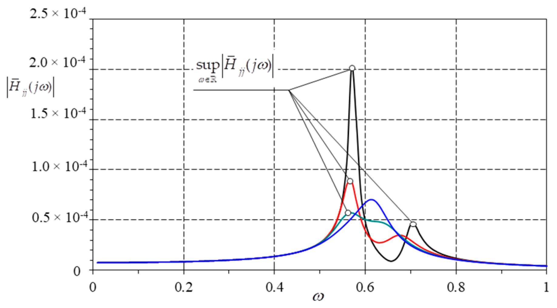
An objective function associated with the ℌ optimization issue was also proposed. In this case, the optimization criterion is the minimization of the maximum values of the FRF | H ( j ω ) | (see Figure 3), which can be described by the formula:
min J 2 = H = sup ω | H ¯ ( j ω ) j j | .
Both cases of the FRF form and optimization included the FRF of the equivalent system | H ¯ ( j ω ) j j | , associated with the j degree of freedom, which was adopted as the equivalent system reduction point, and with the i-th mode of structural natural vibrations and the corresponding value of modal displacement, associated with the primary ordinate q ¯ j i ( t ) = a j i ψ i ( t ) .

2.3. The Issue of Optimization

The analysis used two optimization methods in the form of a standard genetic algorithm (GA), and a simulated annealing (SA) algorithm. Ready libraries for the DELPHI software environment were used.
The procedure for the numerical determination of the optimal parameters can be summed up in the following steps:
  • Calculations of the eigenvalues and eigenvectors in Finite Element (FEM) software, adopting baseline frequency ω i , to which MTMDs will be tuned;
  • Adopting a point for reducing a system to an equivalent SDOF system, normalization of eigenvectors and determination of the parameters for the Equation (7);
  • Adopting a TMD number and initial parameters m k t ,   c k t ,   k k t for the TMDs;
  • Adopting variables, which will be subject to the optimization process, e.g., c k t ,   k k t for a constant value of m k t (different constant parameter options possible);
  • Selection of the optimization method (GA or SA) and the optimization issue, calculations of the equivalent system FRF | H ¯ ( j ω ) j j | , and the determination of values using the Equations (61) or (62) at each optimization step;
  • After reaching the desired calculation accuracy (change of the J1 or J2) value, saving the obtained MTMD parameters, and calculations of the equivalent system FRF | H ¯ ( j ω ) j j | associated with the j degree of freedom, which was adopted as the equivalent system reduction point.

3. Numerical Example 1

3.1. Input Data

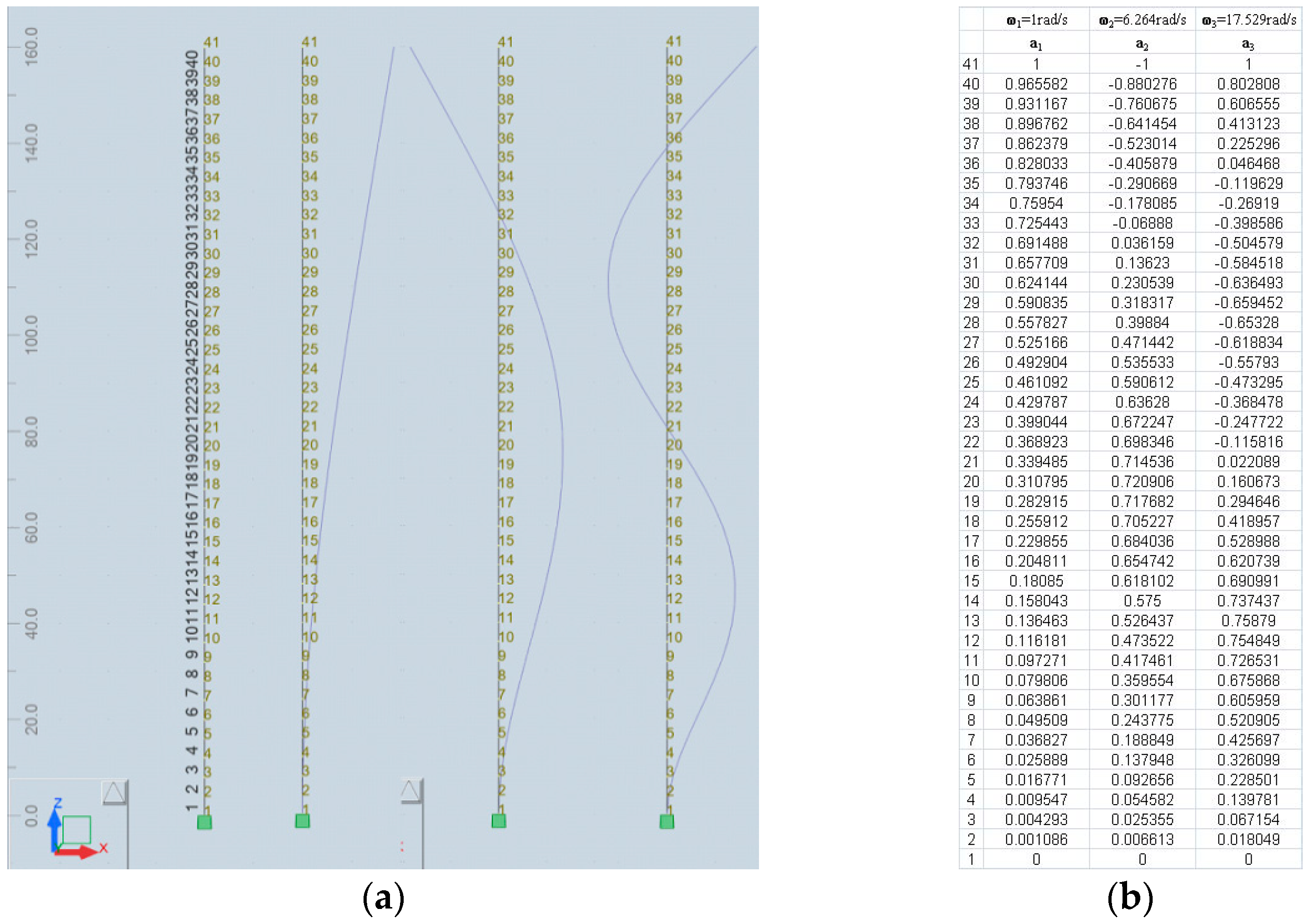
The analysis adopted a cantilever structure in the form of a chimney made of S235 steel, with a height of h=160 m. The chimney parameters were selected so as to obtain the first circular natural frequency equal to ω 1 = 1 rad / s . The chimney diameter and its wall thickness were adopted as a constant, along its entire height. These values equal to, respectively, D = 4010 mm, g = 25.5 mm. The cantilever structure was divided into 40 beam elements with the following parameters: Young modulus E = 210 GPa, Poisson coefficient ν = 0.3, and density ρ = 7850 kg/m3. First three natural vibration modes and their corresponding eigenvalues were calculated. FE software was used to import a normalized eigenvector for the first mode of the natural vibrations, which was then used to construct motion equations for the structure reduced to SDOF system with attached TMD.
Figure 4 shows a FEM model with the numberings of the bars and modes, and a presentation of the first three mode shapes and normalized eigenvectors.
The analysis adopted the issue of tuning TMD and MTMDs to the first natural frequency ω 1 = 1 rad / s . For this frequency, the adopted structural damping was in the form of a damping ratio ζ 1 = 0.02 . The chimney tip (node 41) was selected as the S point for reducing the structure to an SDOF equivalent system. The problem involved finding optimal parameters for a single TMD and MTMDs in the form of 2, 4, 8, and 20 TMDs located also at the place of the highest ordinate of the first vibration mode, which was node 41. New M ¯ , C ¯ , K ¯ matrices for the equivalent system were determined based on the presented modal reduction equations. The equivalent mass determined from the formula m ¯ j i = m ˜ i / a j i 2 = 1 / a j i 2 (where j is the system point of reduction, namely, node 41, whereas i = 1 corresponds to the first natural vibration mode) amounted to m ¯ 41 , 1 = m ˜ 1 / a 41 , 1 2 = 10 5   kg , equivalent stiffness was k ¯ 41 , 1 = k ˜ 1 / a 41 , 1 2 = 100 kN / m , and equivalent damping was c ¯ 41 , 1 = c ˜ 1 / a 41 , 1 2 = 2 ζ 1 ω 1 / a 41 , 1 2 = 4 × 10 3   kg / s . Numerical optimization was conducted for all cases. For each case, the total MTMD mass was equal to the mass of the single TMD, which was adopted as equal to m 1 t = 2 × 10 3   kg . Therefore, the mass factor was μ = m 1 t / m ¯ 41 , 1 = 0.02 . For all other cases, TMD masses were determined from the formula m k t = μ m ¯ 41 , 1 / N k . The natural circular frequency for a single TMD was determined from the formula ω k t = k k t / m k t , whereas the damping factor values for individual TMDs were determined from the formula c k t = 2 ζ k t m k t ω k . Stiffness k k t was used to determine the dimensionless tuning ratio for a single TMD β k = ω k t / ω 1 . Initial tuning adopted for all dampers within the optimization amounted to β k = 1 . This constituted a base to adopt the starting values k k t . Table 1 shows the adopted constant masses of a single TMD and the adopted starting values of the k k t and ζ k t MTMD parameters (values subject to optimization), depending on the TMD number.
The calculation process involved using the aforementioned GA and SA optimization methods and the objective functions based on ℌ2 and ℌ norms in the form of J1 and J2. The frequency range when determining the objective function was (0.0 rad/s:π rad/s).

3.2. Numerical Optimization Results—Comparison of the GA and SA Heuristic Methods

Both heuristic methods do not guarantee finding an exact solution, which is the consequence of the very specificity of the methods. The optimization procedures GA and SA were validated on the 1TMD, 2TMD, and 4TMD models. The parameters of stiffness and damping ratio obtained from both GA and SA optimization methods did not differ. Additionally, both methods were compared for the case of 10TMD (Zuo and Nayfeh [20]) attached to an undamped primary system. Figure 5 shows the optimal TMD parameter values obtained using both methods. Compared to SA, the GA method did not provide results convergent with the results presented in the work by Zuo and Nayfeh [20], while the obtained values of TMDs’ parameters form SA were completely convergent. Unfortunately, with a greater number of optimization variables, the GA algorithm was less stable than the SA algorithm. The obtained results are discussed in greater detail in Section 5. Only the SA optimization method was applied in the further part of the optimization calculations.

3.3. Numerical Optimization Results—SA Method

Optimal MTMD parameters, which are discussed below, were obtained as a result of computations. Table 2 shows the end values of the J1 and J2 objective functions, after the completion of the SA optimization process, using the J1 and J2 objective functions. In addition, it also specifies the percentage change of the objective function value, relative to a 1TMD system. Computation accuracy was adopted at a level of 10−10.
Table 3 and Table 4 show optimal MTMD parameters obtained with optimized J1 and J2 objective functions. A tabular presentation of the 20 TMDs was omitted due to the high number of the results. Results for these cases are shown as drawings in the next section. Figure 6a shows a graph of the FRF module for an equivalent system | H ¯ 41 , 41 | , for a different number of TMDs, and with applied J1 objective function, while Figure 6b shows the same for the J2 objective function.

3.4. Impact of Primary System Mistuning

The analysis also covered the impact by the changing mass of the equivalent structure m ¯ 41 , 1 , on the value of the equivalent structure FRF | H ¯ 41 , 41 | for a structure with attached MTMDs with optimal parameters, predetermined based on the J1 and J2 objective functions. A 10% reduction and increase in the equivalent structure mass was assumed, which resulted in the change of the natural circular frequencies to a value of ω 1 10 % = 1.05409   rad / s and ω 1 + 10 % = 0.95346   rad / s , respectively. Figure 7a shows a graph of the FRF module for an equivalent system | H ¯ 41 , 41 | , for a mass reduction of 10% and a different number of TMDs, and with applied J1 objective function, while Figure 7b shows the same for the J2 objective function. Figure 8a,b shows analogous graphs but for a mass increase of 10% (designation +10% and −10% means an increase and reduction of the m ¯ 41 , 1 equivalent mass, respectively).

3.5. Discussion

The analyses presented in Section 3 were used as a base to compare the application of the SA optimization method and the J1 and J2 objective functions with known analytical solutions in terms of a single TMD. Table 5 shows known formulas for the determination of the optimal parameters for TMD usually determined from a TDOF system, with stated values of the optimal parameters. The table also presents original results for 1 TMD, taking into account natural damping of the primary system, as well as without it. Figure 8 shows an equivalent system FRF module graph for optimal TMD parameters. When analyzing the obtained solution (see Table 5 and Figure 9a), in the case of no damping of the primary system ζ 1 = 0 and in comparison with the Den Hartog solution [1], which has been known for years, one can state very good conformity of the optimal tuning parameters β 1 and the TMD damping factor ζ 1 t , whereas optimal TMD parameters proposed by Warburton [2], upon a harmonic excitation, are close to the parameters obtained through calculations of the J2 objective function optimization. The solution proposed by Ren [31] suits a different kind of TMD, where the damping element is not connected with the primary mass but with the substrate (other motion equations); hence, it is impossible to directly apply the optimal parameter formulas proposed in this study as parameters for a standard TDOF system. Furthermore, please note that optimal TMD parameters based on the ℌ2 norm (white noise input), i.e., determined from the J1 objective function, provided similar TMD efficiency, as suggested by Warburton in [3].
In the case of an analysis covering a structure including natural damping of the primary system, we can observe that FRF module graphs, developed based on optimal Den Hartog and Warburton parameters, are no longer consistent with the graphs based on the parameters obtained through the ℌ2 and ℌ methods, that is, the J1 and J2 objective functions. This, of course, stems from the fact that these formulas do not include natural damping ζ 1 , whereas, when comparing to the Matsuhis solution [32], where the optimal parameters were obtained based on the stability criterion, taking into account ζ 1 , it should be concluded that his solution was optimal neither for harmonic excitations nor for white noise input.
In [20], Zuo and Nayfeh conducted a free analysis of the β k , ζ k t parameters, with a constant value of m k t , for 10 and 100 TMDs, with not damping of the primary system ζ 1 = 0 and a μ = 0.05 mass ratio. They applied optimization based on the ℌ2 norm and used state space equations for an SDOF system with attached MTMDs. The work also presents tuning increment graphs for individual TMDs in the form of β k β k 1 . The authors of that article also conducted such simulations for n = 10 (number of TMD), ζ 1 = 0 , and μ = 0.05 . Figure 10 shows tuning β k and damping ratio ζ k distribution based on the number of TMDs, while Figure 11 shows tuning increments and tuning factor for individual TMDs in the form of β k β k 1 and ζ k ζ k 1 . The obtained β k , ζ k t and β k β k 1 parameters exhibited very good conformity with the results of Zuo and Nayfeh [20].
In the course of analyzing the results shown in Section 3, which concern the optimization of MTMDs located at the tip of a h = 160-m-high chimney, higher effectiveness of MTMDs relative to a single TMD can be confirmed (see Table 2 and Figure 6). This is particularly clear to optimal parameters determined with the J2 objective function, where the location of the flat section of graph | H ¯ 41 , 41 | in the area of ω 1 can be seen increasingly lower (Figure 6b). Another issue that needs to be stressed are the graphs | H ¯ 41 , 41 | (Figure 6a) for TMD tuning in the form of white noise ℌ2 optimization of the J1 function exhibit a broader damper impact range on the side of higher input frequencies.
Furthermore, Figure 12 shows a function variability graph depending on the number of TMDs. Of course, higher MTMD efficiency relative to TMDs can be observed for both objective functions, J1 and J2, applied within the numerical optimization. Furthermore, Figure 12 shows the values of individual objective functions for the optimal parameters obtained using both optimization methods, namely, ℌ2 (J1 function) and ℌ (J2 function). It can be seen (see Figure 12a) that in the case of random excitation, which corresponds to the value of the J1 function and TMDs tuned to harmonic excitation (optimal parameters based on the optimization of function J2), we get a lower MTMD efficiency. Figure 12b indicates an inverse relationship.
When analyzing the results concerning the primary system mass change (see Figure 7 and Figure 8), for an approximately 5% difference in the value of ω 1 (“structural mistuning”), MTMDs are more effective than a single TMD. A lower effectiveness with a higher number of TMDs tuned to harmonic excitations can be observed only in the case of TMDs tuned based on J2 optimization and reducing the primary system mass increase in frequency ω 1 10 % = 1.05409   rad / s . In the event of such a primary system mistuning, better effectiveness was exhibited by MTMDs tuned based on J1, which resulted from the aforementioned broadband excitation on the side of frequencies higher than ω 1 . It can also be concluded that a reduction in the primary system mass had a more adverse influence on the structural response and MTMD operation than mass increase. These relationships are shown in Figure 13. It can also be assumed that with a low difference (below 5%) between the calculated natural frequencies of the structure and the ones determined for a real structure, it is advisable to use MTMDs instead of a single TMD. The aforementioned analyses confirm the general conclusions included in the works by Zuo and Nayfeh [20] as well as Li and Ni [21] concerning the higher effectiveness of MTMDs relative to TMDs.
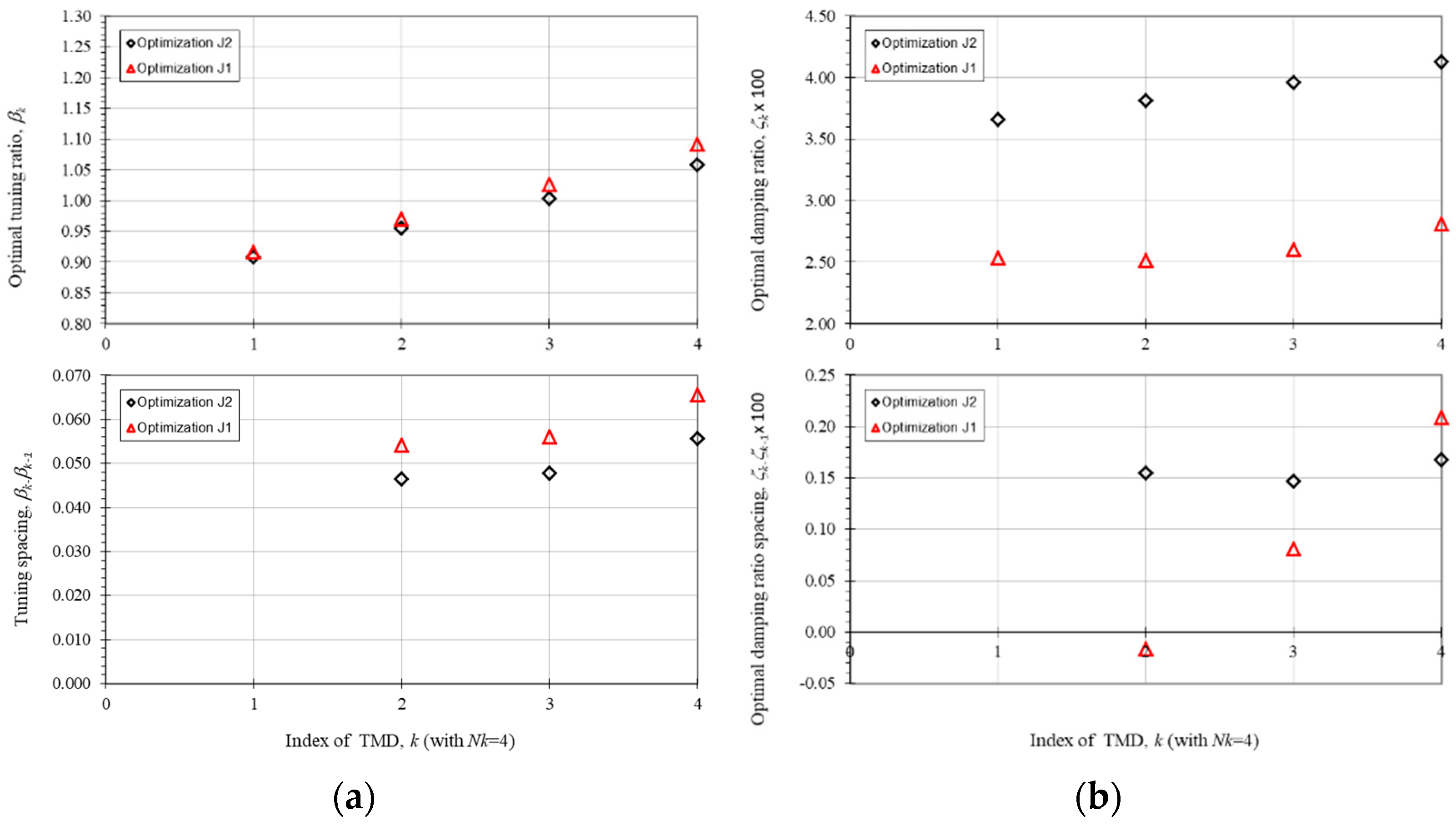
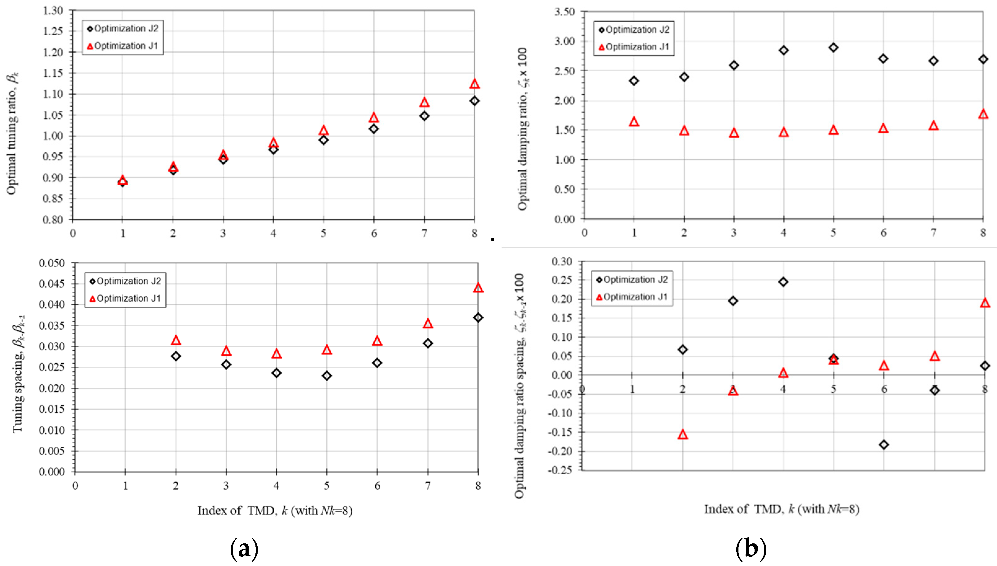
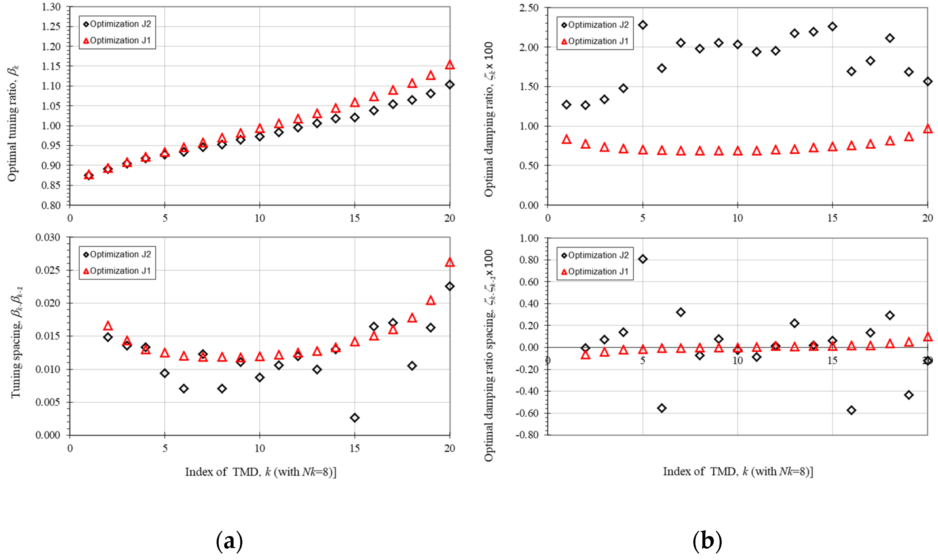
Additionally, for analysis purposes, it was decided to present the results of optimal MTMD parameters in the form of optimal tuning ratio β k and optimal damping ratio ζ k t graphs depending on the number of TMDs. The tuning and damping factor increments for individual TMDs in the form of β k β k 1 and ζ k t ζ k 1 t were also presented. After a thorough review of the graphs (see Figure 14, Figure 15 and Figure 16) presented for cases with 4, 8, and 20 TMDs, conclusions can be drawn regarding the application of the J1 objective function based on the ℌ2 norm and the J2 function based on the ℌ norm. As far as the tuning distribution is concerned, we can observe increased factor β k for TMDs tuned above and below the ω 1 frequency. The area of TMDs tuned to values beyond ω 1 exhibited a significantly higher growth of the value β k , especially for the parameters obtained from the J1 objective function, which is particularly well illustrated by the graphs β k β k 1 . If we consider the optimal tuning ratio graphs for individual ζ k t , we can observe a derivative characteristic, but only for the J1 function, although the increments ζ k t ζ k 1 t no longer show a similar dependency as β k β k 1 . On the other hand, the optimal parameters ζ k t obtained based on the J2 function look completely different. In this case, the graph shows a significant drop in the ζ k t values for “central” TMDs tuned on ω 1 .

4. Numerical Example 2

4.1. Input Data

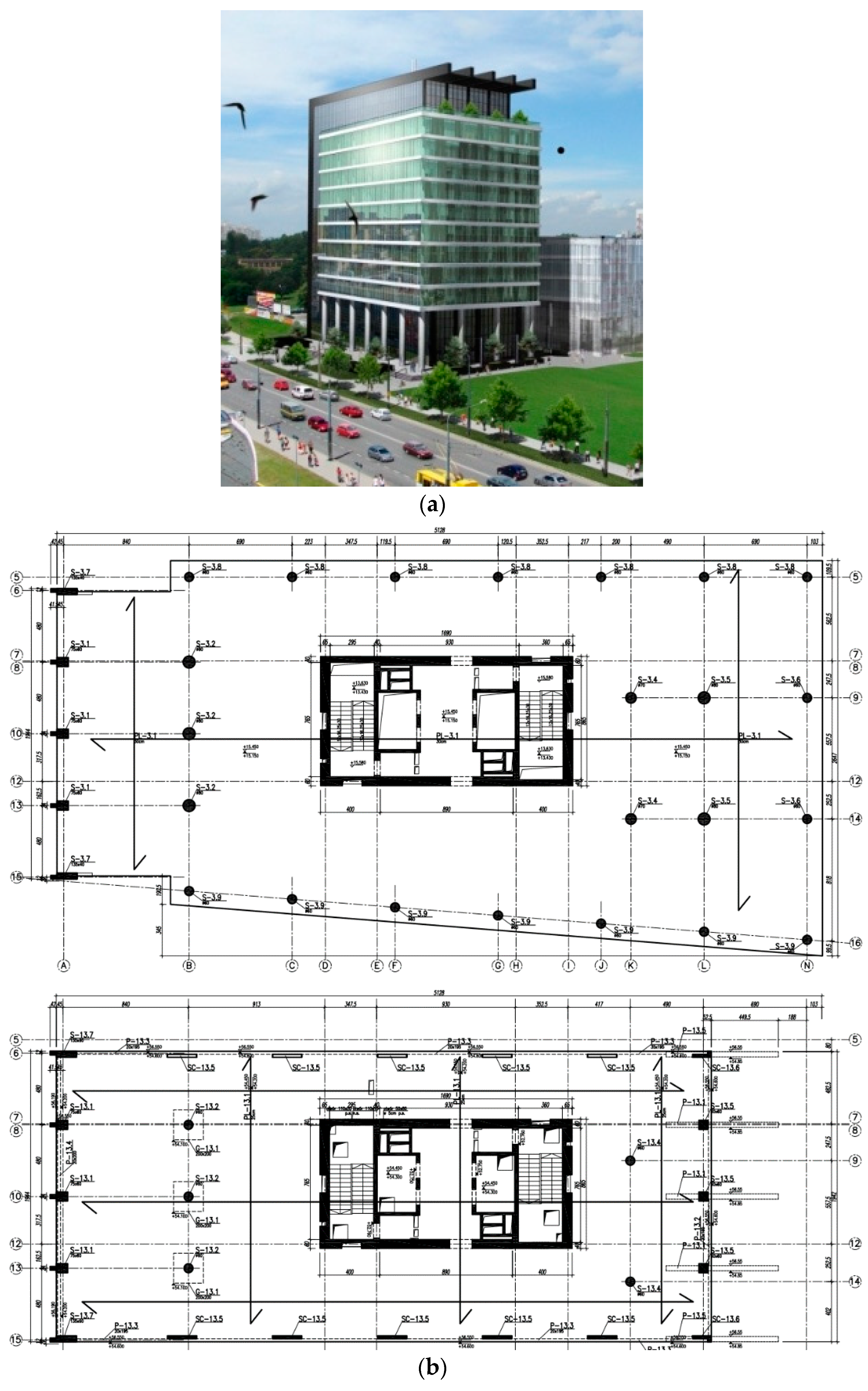
The next analysis is an example of the optimization of MTMD mounted on a complex, reinforced concrete structure in the form of a tall building. The analysis included Gray Office “A” located in the city of Lublin in Poland. The building is set on a foundation slab with two underground and 13 aboveground stories. The heights of the underground stories are 3.5 m and the overground stories are 3.9 m. The total height of the building is 56.55 m. Figure 17a shows the architectural visualization of the building, while Figure 17b shows the structural plans of floors 3 and 13. The main load-bearing system is the reinforced concrete core of the building (modified for the present analysis by adding walls in the E-H axes), with wall thicknesses from 20 cm to 65 cm. The remaining load-bearing structure is a reinforced concrete slab ceiling (ceilings thickness from 25 cm to 45 cm), based on reinforced concrete pillars of various dimensions from 60–100 cm.
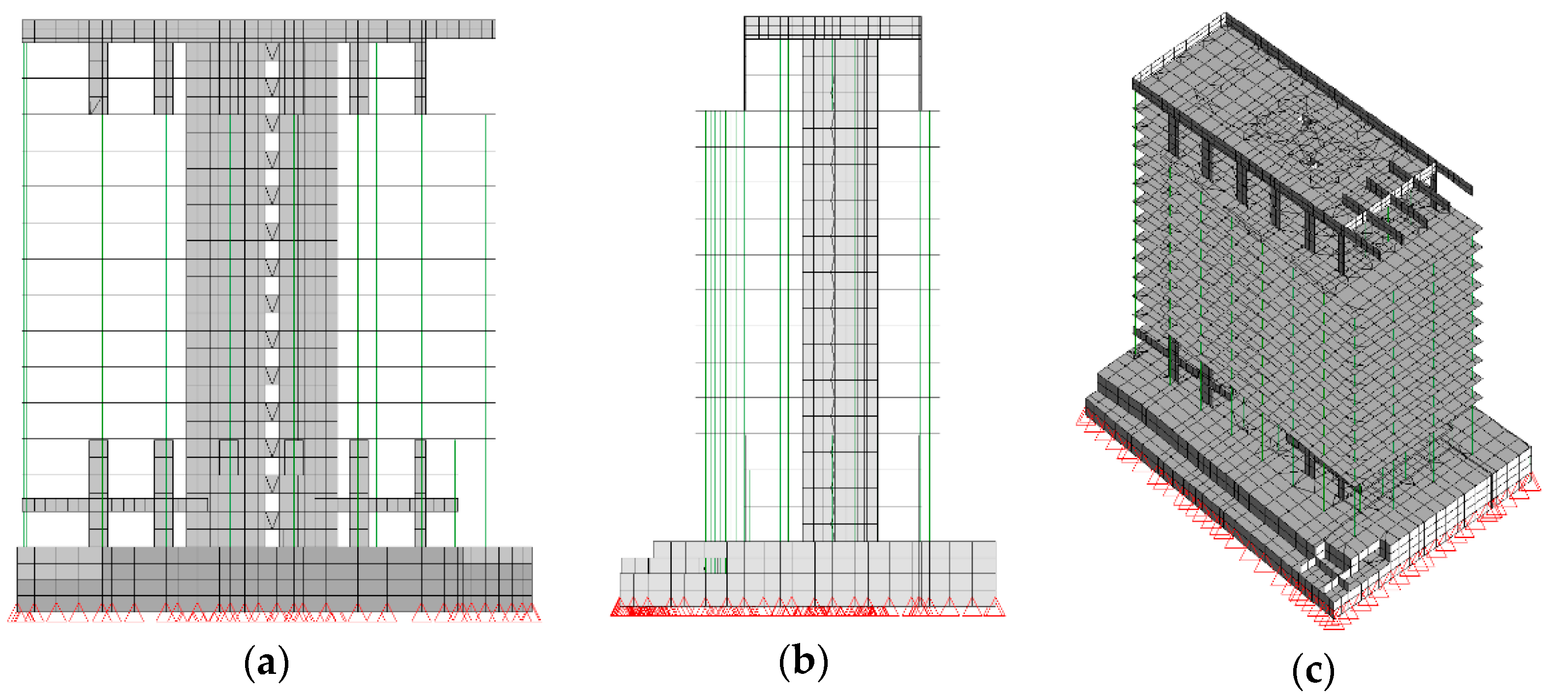
Figure 18 shows the FEM model of the system. The used beam and shell elements with concrete parameters C25/C30 are Young modulus E = 32 GPa, Poisson coefficient ν = 0.2, and density ρ = 2870 kg/m3 (increasing the density to accommodate the flooring layers). The number of nodes in the model was 11,894, and the total number of equations in the modal analysis was 69,912.
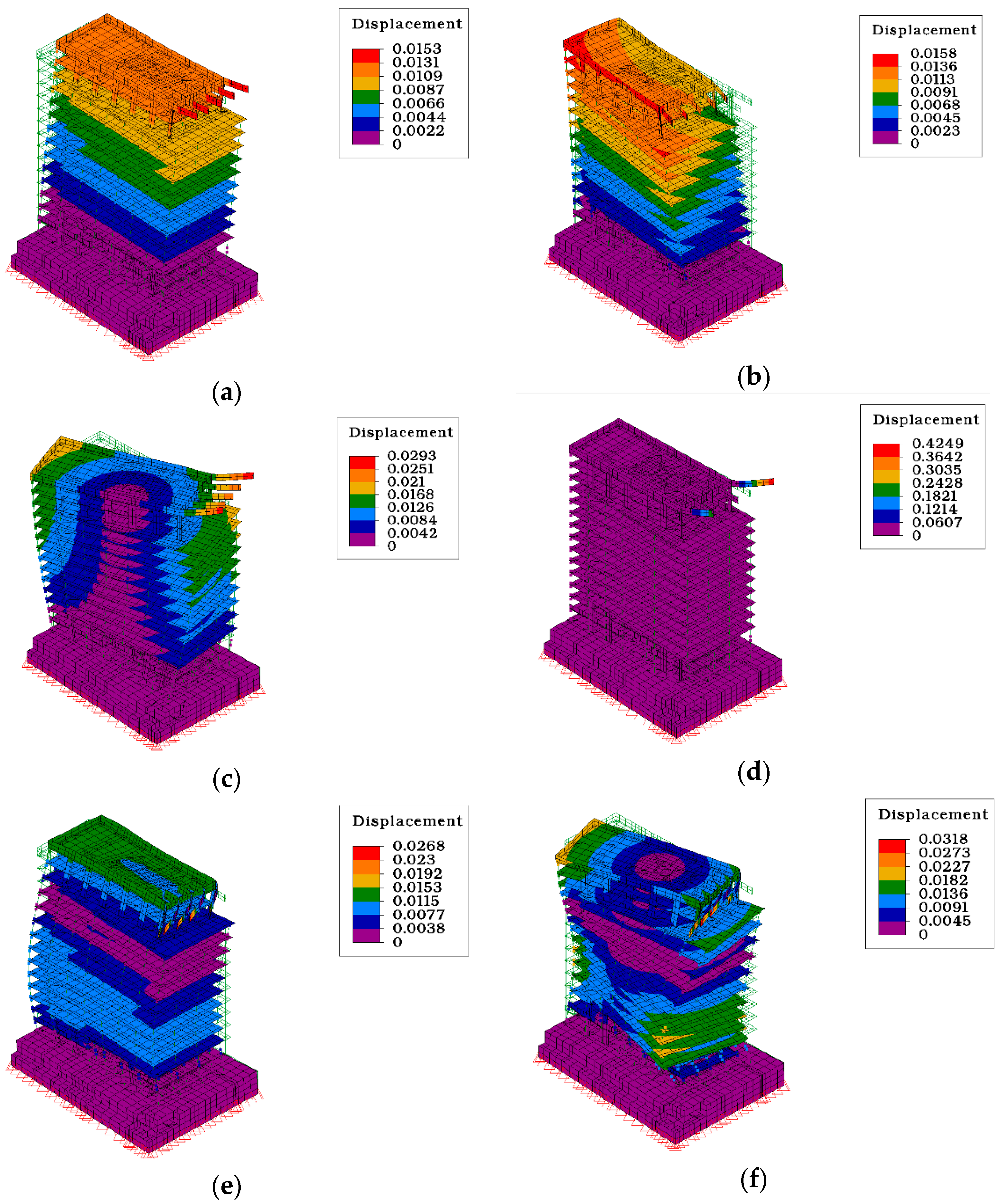
The first 11 corresponding natural vibration modes and their eigenvalues were calculated. Table 6 presents the description of particular modes of vibration below the value of f < 5 Hz, while Figure 19 shows selected modes’ shapes, disregarding the local natural frequencies (f4 to f8) of the cantilever beams located on the last floor of the building. The frequencies of natural vibrations were separated. The first flexural form of natural vibrations in the Y direction corresponded to f1 = 0.8431 Hz, and the next bending form of vibrations occurred at the frequency f2 = 1.3476 Hz. FE software was used to import a normalized eigenvector for the first mode of the natural vibrations, which was then used to construct motion equations for the structure reduced to SDOF system with attached TMDs.
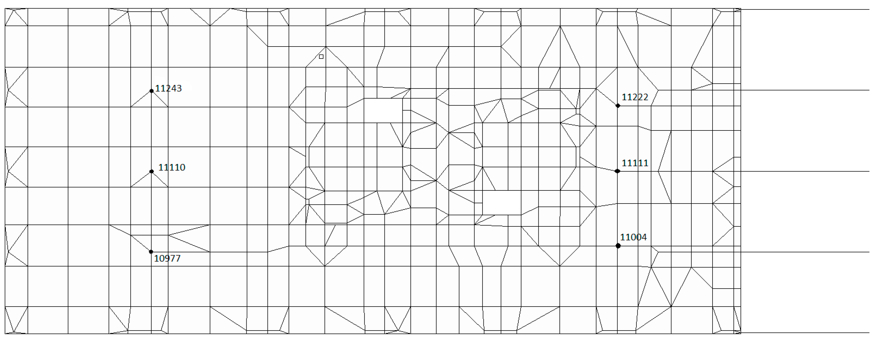
The analysis adopted the issue of tuning MTMD to the first natural frequency f1 = 0.8431 Hz. The damping value was assumed in the form of a logarithmic damping decrement δ = 0.08. Node 11,110 was accepted was selected as the S point for reducing the structure to an SDOF equivalent system. The problem involved finding optimal parameters for MTMDs in the form of 2, 4, and 6 TMDs located on the ceiling of the top floor. There were three cases of TMDs attachment: 2 TMDs, at nodes 11,110 and 11,111; 4 TMDs, at nodes 11,243, 10,977, 11,222, and 11,004; 6 TMDs, at nodes 11,243, 11,110, 10,977, 11,222, 11,111, and 11004. The Y direction was adopted as the operating direction of all TMDs. The designations of the nodes are shown in Figure 20.
New M ¯ , C ¯ , K ¯ matrices for the equivalent system were determined based on the presented modal reduction equations. The equivalent mass determined from the formula m ¯ j i = m ˜ i / a j i 2 = 1 / a j i 2 (where j is the system point of reduction, namely, node 11,110, whereas i = 1 corresponds to the first natural vibration mode) amounted to m ¯ 11110 , 1 = m ˜ 1 / a 11110 , 1 2 = 6.7449 × 10 6   kg , equivalent stiffness was k ¯ 11110 , 1 = k ˜ 1 / a 11110 , 1 2 = ω 1 2 / a 11110 , 1 2 = 1.8909 × 10 5 kN / m , and equivalent damping was c ¯ 11110 , 1 = c ˜ 1 / a 11110 , 1 2 = 2 ζ 1 ω 1 / a 11110 , 1 2 = 9.09 × 10 2   kg / s . Numerical optimization was conducted for all cases. For each case, the total MTMD stiffness was equal to the stiffness of the 1 TMD, which was adopted as equal to k 1 t = 120 kN / m . For all other cases, TMDs’ stiffness was determined from the formula k k t = k 1 t / N k . In the optimization process, the variables were the mass m k t and the damping ratio ζ k t .
The calculation process involved using the aforementioned SA optimization methods and the objective functions based on ℌ2 and ℌ norms in the form of J1 and J2.

4.2. Numerical Optimization Results and Discussion

Optimal MTMD parameters were obtained as a result of computations. Table 7 and Table 8 show optimal MTMD parameters obtained with optimized J1 and J2 objective functions. Figure 21 shows plots of the FRF module for node 11,110 for X and Y direction, respectively (for original system with a different number of TMDs and J1 optimization), while Figure 22 shows the same FRF module plots for the J2 objective function. From the analysis of plots of the FRF module (Figure 21 and Figure 22), it can be seen that for the X direction, we did not observe changes in the FRF module value, while for the Y direction, we observed a decrease in the FRF module value in the first natural frequency range f1 = 0.8431 Hz. Additionally, we can observe that the vibration frequencies f4 to f8 are not visible on the FRF module plots.
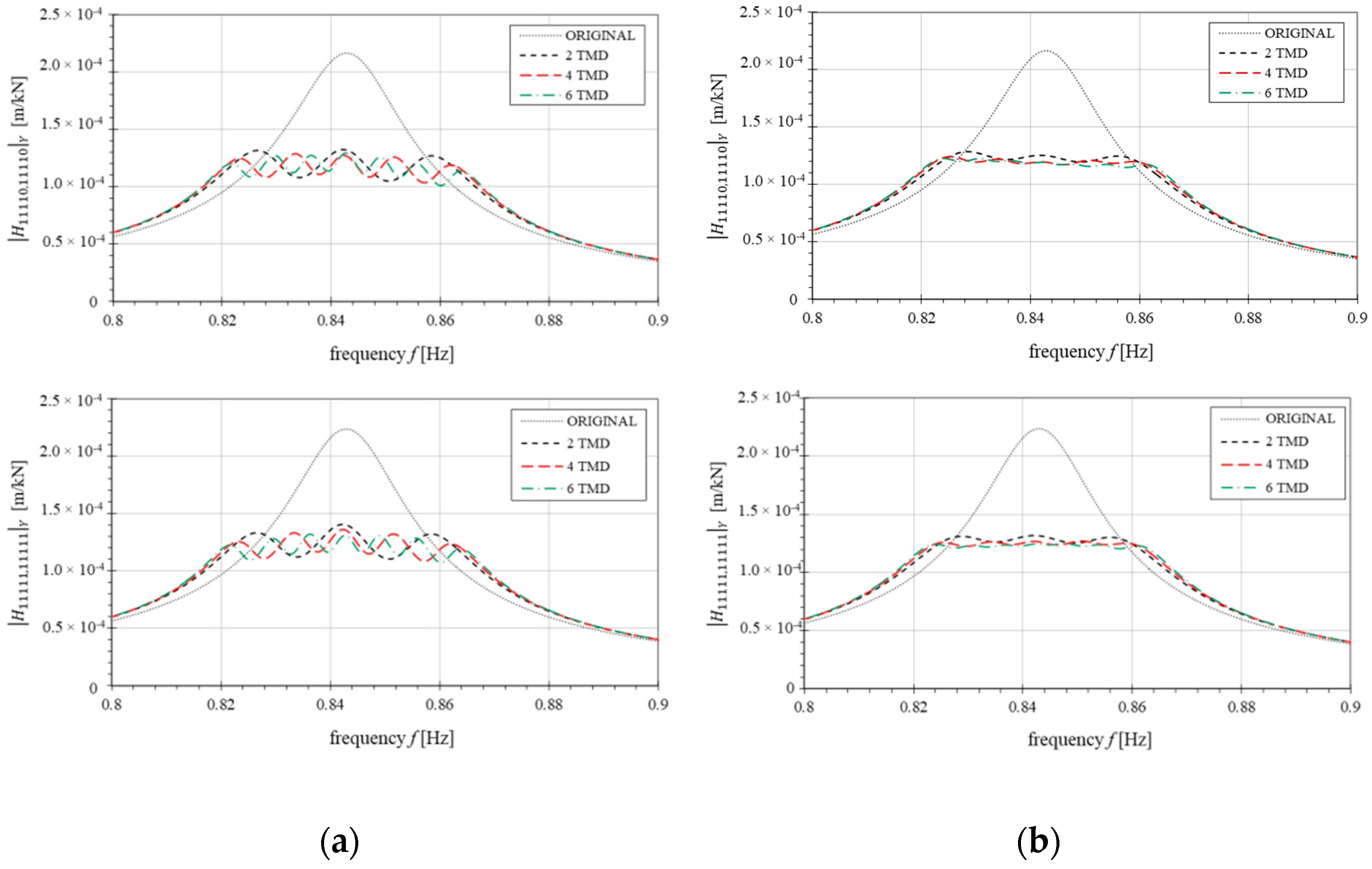
Figure 23 shows the FRF module in the Y direction for two nodes, 11,110 and 11,111, in the frequency range 0.8 Hz to 0.9 Hz. As in the previous example, the same nature of the FRF module plots for the optimal TMD parameters obtained from the functions J1 and J2 can be observed. However, it should be borne in mind that the optimization process was carried out on the equivalent displacement of the SDOF system, while the FRF module plots were presented for the original system with thousands of DOF. The presented graphs also show the fact of greater efficiency of MTMD with an increasing number of TMDs.

5. Conclusions

The adopted novel method for developing motion equations enables adding single TMDs or MTMDs to completely different degrees of freedom of the primary system. The system of equations allows for easy MTMD tuning for complex vibrations modes, with MTMDs located in local maxima of these vibrations’ modes, while still analyzing the SDOF system with attached MTMDs. Locating MTMDs at the tip of the chimney provided a possibility to compare the results with studies on MTMD tuning. The next stage of the research was to optimize MTMD parameters in a complex structure, but still analyze as an SDOF system. Of course, the thesis of better effectiveness of MTMD over a single TMD was confirmed.
Based on conducted analysis, it was observed that the k k t , ζ k t free optimization was of completely different nature in the case of optimizations based on the ℌ2 and ℌ norms, especially for the ζ k t parameters, where the ζ k t ζ k 1 t increments showed totally different forms for both J1 and J2 objective functions.

Author Contributions

Conceptualization, P.W. and R.G.; formal analysis, P.W.; investigation, P.W.; methodology, P.W. and R.G.; resources, P.W.; software, P.W.; supervision, P.W.; validation, R.G.; visualization, R.G.; writing original draft, P.W.; writing review and editing, R.G. All authors have read and agreed to the published version of the manuscript.

Funding

This research was funded by the Science Financing Subsidy Lublin University of Technology (FN16/ILT/2020).

Institutional Review Board Statement

Not applicable.

Informed Consent Statement

Not applicable.

Data Availability Statement

Data available on request due to restrictions e.g., privacy or ethical.

Conflicts of Interest

The authors declare no conflict of interest.

References

  1. Den Hartog, J.P.D. Mechanical Vibration; McGraw-Hill: New York, NY, USA, 1956. [Google Scholar]
  2. Warburton, G.B. Optimum absorber parameters for various combinations of response and excitation parameters. Earthq. Eng. Struct. Dyn. 1982, 10, 381–401. [Google Scholar] [CrossRef]
  3. Warburton, G.B. Optimum absorber parameters for minimizing vibration response. Earthq. Eng. Struct. Dyn. 1981, 9, 251–262. [Google Scholar] [CrossRef]
  4. Bakre, S.V.; Jangid, R.S. Optimum parameters of tuned mass damper for damped main system. Struct. Control Health Monit. 2007, 14, 448–470. [Google Scholar] [CrossRef]
  5. Bakre, S.V.; Jangid, R.S. Optimum multiple tuned mass dampers for base-excited damped main system. Int. J. Struct. Stab. Dyn. 2004, 4, 527–542. [Google Scholar] [CrossRef]
  6. Krenk, S. Frequency analysis of the tuned mass damper. J. Appl. Mech. Trans. ASME 2005, 72, 936–942. [Google Scholar] [CrossRef]
  7. Batou, A.; Adhikari, S. Optimal parameters of viscoelastic tuned-mass dampers. J. Sound Vib. 2019, 445, 17–28. [Google Scholar] [CrossRef] [Green Version]
  8. Marian, L.; Giaralis, A. The tuned mass-damper-inerter for harmonic vibrations suppression, attached mass reduction, and energy harvesting. Smart Struct. Syst. 2017, 19, 665–678. [Google Scholar] [CrossRef]
  9. Sentyakov, K.; Peterka, J.; Smirnov, V.; Bozek, P.; Sviatskii, V. Modeling of boring mandrel working process with vibration damper. Materials 2020, 13, 1931. [Google Scholar] [CrossRef] [Green Version]
  10. Bergman, L.A.; McFarland, D.M.; Hall, J.K.; Johnson, E.A.; Kareem, A. Optimal distribution of tuned mass dampers in wind-sensitive structures. In Proceedings of the ICOSSAR ’89, the 5th International Conference on Structural Safety and Reliability, Part I, San Francisco, CA, USA, 7–11 August 1989; ASCE: New York, NY, USA, 1989; pp. 95–102. [Google Scholar]
  11. Kareem, A.; Kline, S. Performance of Multiple Mass Dampers under Random Loading. J. Struct. Eng. 1995, 121, 348–361. [Google Scholar] [CrossRef]
  12. Igusa, T.; Xu, K. Vibration Control Using Multiple Tuned Mass Dampers. J. Sound Vib. 1994, 175, 491–503. [Google Scholar] [CrossRef]
  13. Joshi, A.S.; Jangid, R.S. Optimum parameters of multiple tuned mass dampers for base-excited damped systems. J. Sound Vib. 1997, 202, 657–667. [Google Scholar] [CrossRef]
  14. Jangid, R.S. Optimum Multiple Tuned Mass Dampers for base-excited undamped system. Earthq. Eng. Struct. Dyn. 1999, 28, 1041–1049. [Google Scholar] [CrossRef]
  15. Yamaguchi, H.; Harnpornchai, N. Fundamental characteristics of Multiple Tuned Mass Dampers for suppressing harmonically forced oscillations. Earthq. Eng. Struct. Dyn. 1993, 22, 51–62. [Google Scholar] [CrossRef]
  16. Zuo, L.; Nayfeh, S.A. The two-degree-of-freedom tuned-mass damper for suppression of single-mode vibration under random and harmonic excitation. J. Vib. Acoust. Trans. ASME 2006, 128, 56–65. [Google Scholar] [CrossRef]
  17. Zhao, G.; Raze, G.; Paknejad, A.; Deraemaeker, A.; Kerschen, G.; Collette, C. Active tuned inerter-damper for smart structures and its optimisation. Mech. Syst. Signal Process. 2019, 129, 470–478. [Google Scholar] [CrossRef] [Green Version]
  18. Aggumus, H.; Guclu, R. Robust H∞ control of STMDs used in structural systems by hardware in the loop simulation method. Actuators 2020, 9, 55. [Google Scholar] [CrossRef]
  19. Asami, T. Optimal Design of Double-Mass Dynamic Vibration Absorbers Arranged in Series or in Parallel. J. Vib. Acoust. 2017, 139. [Google Scholar] [CrossRef]
  20. Zuo, L.; Nayfeh, S.A. Optimization of the individual stiffness and damping parameters in multiple-tuned-mass-damper systems. J. Vib. Acoust. Trans. ASME 2005, 127, 77–83. [Google Scholar] [CrossRef]
  21. Li, H.N.; Ni, X.L. Optimization of non-uniformly distributed multiple tuned mass damper. J. Sound Vib. 2007. [Google Scholar] [CrossRef]
  22. Zuo, L.; Nayfeh, S.A. Minimax optimization of multi-degree-of-freedom tuned-mass dampers. J. Sound Vib. 2004, 272, 893–908. [Google Scholar] [CrossRef]
  23. Ok, S.Y.; Song, J.; Park, K.S. Optimal design of hysteretic dampers connecting adjacent structures using multi-objective genetic algorithm and stochastic linearization method. Eng. Struct. 2008, 30, 1240–1249. [Google Scholar] [CrossRef]
  24. Leung, A.Y.T.; Zhang, H. Particle swarm optimization of tuned mass dampers. Eng. Struct. 2009, 31, 715–728. [Google Scholar] [CrossRef]
  25. Zhang, R.; Zhang, Y.; Zheng, Z.; Mo, L.; Wu, C. Parametrical optimization of particle dampers based on particle swarm algorithm. Appl. Acoust. 2020, 160, 107083. [Google Scholar] [CrossRef]
  26. Aydin, E.; Öztürk, B.; Dutkiewicz, M. Analysis of efficiency of passive dampers in multistorey buildings. J. Sound Vib. 2019, 439, 17–28. [Google Scholar] [CrossRef]
  27. Kim, S.Y.; Lee, C.H. Optimum design of linear multiple tuned mass dampers subjected to white-noise base acceleration considering practical configurations. Eng. Struct. 2018. [Google Scholar] [CrossRef]
  28. Stanikzai, M.H.; Elias, S.; Matsagar, V.A.; Jain, A.K. Seismic response control of base-isolated buildings using tuned mass damper. Aust. J. Struct. Eng. 2019. [Google Scholar] [CrossRef]
  29. Yin, X.; Song, G.; Liu, Y. Vibration Suppression of Wind/Traffic/Bridge Coupled System Using Multiple Pounding Tuned Mass Dampers (MPTMD). Sensors 2019, 19, 1133. [Google Scholar] [CrossRef] [Green Version]
  30. Bendat, J.S.; Piersol, A.G. Random Data; Wiley Series in Probability and Statistics; John Wiley & Sons, Inc.: Hoboken, NJ, USA, 2010; ISBN 9781118032428. [Google Scholar]
  31. Ren, M.Z. A variant design of the dynamic vibration absorber. J. Sound Vib. 2001, 245, 762–770. [Google Scholar] [CrossRef]
  32. Nishihara, O.; Matsuhisa, H. Design of a dynamic vibration absorber for minimization of maximum amplitude magnification factor (Derivation of algebraic exact solution). Jpn. Soc. Mech. Eng. 1997, 63, 3438–3445. [Google Scholar] [CrossRef] [Green Version]
Figure 1. The primary system, adopted first, and i-th mode shape, together with an SDOF equivalent system.
Applsci 11 01389 g001
Figure 2. General arrangement diagram for tuned mass dampers (TMDs) within the main structure.
Applsci 11 01389 g002
Figure 3. Objective function J2 determination diagram (maximum value).
Applsci 11 01389 g003
Figure 4. (a) Finite Element Method (FEM) model of the chimney and the first three mode shapes; (b) normalized eigenvectors for the first three eigenvalues.
Applsci 11 01389 g004
Figure 5. (a) Optimal tuning ratios β k ; (b) optimal damping ratios ζ k t of the individual TMD for μ = 0.05 and ζ 1 = 0 for SA and GA method.
Applsci 11 01389 g005
Figure 6. Module graph of a FRF | H ¯ 41 , 41 | for optimal parameters and a different number of TMDs: (a) for the J1 objective function; (b) for the J2 objective function.
Applsci 11 01389 g006
Figure 7. Module graph of a FRF | H ¯ 41 , 41 | with the mass of the primary system reduced by 10% for optimal parameters and a different number of TMDs: (a) for the J1 objective function; (b) for the J2 objective function.
Applsci 11 01389 g007
Figure 8. Module graph of a FRF | H ¯ 41 , 41 | with the mass of the primary system increased by 10% for optimal parameters and a different number of TMDs: (a) for the J1 objective function; (b) for the J2 objective function.
Applsci 11 01389 g008
Figure 9. The module graph for the FRF | H ¯ 41 , 41 | (value corresponds to the FRF | H 1 , 1 | of a two degree of freedom (TDOF) system based on various studies): (a) case ζ 1 = 0 ; (b) case ζ 1 = 0.02 .
Applsci 11 01389 g009
Figure 10. Optimal tuning ratios β k and damping ratios ζ k t of the individual TMD for μ = 0.05 and ζ 1 = 0 obtained on the basis of J1.
Applsci 11 01389 g010
Figure 11. Optimal tuning spacings β k β k 1 and damping ratios spacings ζ k ζ k 1 of the individual TMD for μ = 0.05 and ζ 1 = 0 obtained on the basis of J1.
Applsci 11 01389 g011
Figure 12. Objective function values based on the optimal parameters obtained from J1 and J2, depending on the number of TMDs: (a) value of J1; (b) value of J2.
Applsci 11 01389 g012
Figure 13. Objective function value, in the case of primary system mistuning (10% increase and drop of mass), based on the optimal parameters obtained from J1 and J2, depending on the number of TMDs: (a) value of J1; (b) value of J2.
Applsci 11 01389 g013
Figure 14. (a) Optimal tuning ratios β k and optimal tuning spacings β k β k 1 ; (b) optimal damping ratios ζ k t and damping ratios’ spacings ζ k ζ k 1 of the individual TMD for N k = 4 , μ = 0.02 , and ζ 1 = 0.02 .
Applsci 11 01389 g014
Figure 15. (a) Optimal tuning ratios β k and optimal tuning spacings β k β k 1 ; (b) optimal damping ratios ζ k t and damping ratios’ spacings ζ k ζ k 1 of the individual TMD for N k = 8 , μ = 0.02 , and ζ 1 = 0.02 .
Applsci 11 01389 g015
Figure 16. (a) Optimal tuning ratios β k and optimal tuning spacings β k β k 1 ; (b) optimal damping ratios ζ k t and damping ratios’ spacings ζ k ζ k 1 of the individual TMD for N k = 20 , μ = 0.02 , and ζ 1 = 0.02 .
Applsci 11 01389 g016
Figure 17. (a) Visualization of a tall building: (b) structural plan of floors 2 and 13 (top floor of the building).
Applsci 11 01389 g017
Figure 18. FEM model of the structure: (a) front view; (b) side view; (c) axonometric view.
Applsci 11 01389 g018
Figure 19. Mode shapes of natural vibrations for frequencies: (a) f1 = 0.8431 Hz; (b) f2 = 1.3476 Hz; (c) f3 = 1.4488 Hz; (d) f5 = 2.5222 Hz; (e) f9 = 4.0457 Hz; (f) f10 = 4.3516 Hz.
Applsci 11 01389 g019
Figure 20. FEM model of the last floor ceiling with the numbers of nodes in which the TMDs’ location was assumed.
Applsci 11 01389 g020
Figure 21. Module graph of the FRF in node 11,110 for optimal TMD parameters (J1) and a different number of TMDs: (a) for X direction; (b) for Y direction.
Applsci 11 01389 g021
Figure 22. Module graph of the FRF in node 11,110 for optimal TMD parameters (J2) and a different number of TMDs: (a) for X direction; (b) for Y direction.
Applsci 11 01389 g022
Figure 23. Module graph of a FRF in node 11,110 and 11,111 for optimal parameters and a different number of TMDs: (a) for the J1 objective function; (b) for the J2 objective function.
Applsci 11 01389 g023
Table 1. Mass values for individual TMDs and k k t and ζ k t starting values.
TMD Number m k t k k t ζ k t
[kg][kN/m][–]
1 TMD20002.000.05
2 TMDs10001.000.05
4 TMDs5000.500.05
8 TMDs2500.250.05
20 TMDs1000.100.05
Table 2. The value of the J1 and J2 functions after completed optimization with the SA method.
TMD NumberJ1 ValueJ1 ChangeJ2 ValueJ2 Change
[m/(kN*s^0.5)][%][m/kN][%]
SDOF2.4910 × 10−2 2.5005 × 10⁻¹
1 TMD1.5515 × 10−20.00%7.4579 × 10−20.00%
2 TMDs1.5203 × 10−2−2.01%6.8248 × 10⁻²−8.49%
4 TMDs1.5001 × 10−2−3.31%6.4091 × 10⁻²−14.06%
8 TMDs1.4875 × 10−2−4.12%6.1620 × 10⁻²−17.38%
20 TMDs1.4783 × 10−2−4.72%6.0202 × 10⁻²−19.28%
Table 3. Optimal k k t , ζ k t , β k values obtained for the J1 objective function.
MTMDNo. m k t k k t ζ k t β k
[kg][kN/m][–][–]
1 TMD120001.9609050.0684620.990178
2 TMDs110000.8954980.0416050.946307
210001.0966140.0443811.047193
4 TMDs15000.4194780.0253490.915945
25000.4704540.0251860.970004
35000.5264160.0259981.026076
45000.5958900.0280821.091687
8 TMDs12500.2003530.0165360.895215
22500.2147380.0149900.926796
32500.2284310.0145930.955889
42500.2422030.0146690.984282
52500.2568580.0150861.013624
62500.2730790.0153561.045139
72500.2919740.0158771.080691
82500.3162990.0177891.124809
Table 4. Optimal k k t , ζ k t , β k values obtained for the J2 objective function.
MTMDNo. m k t k k t ζ k t β k
[kg][kN/m][–][–]
1 TMD120001.9058200.0891690.976171
2 TMDs110000.8786970.0562780.937388
210001.0462570.0629211.022867
4 TMDs15000.4131070.0366080.908964
25000.4564090.0381550.955415
35000.5032230.0396211.003218
45000.5606260.0412951.058892
8 TMDs12500.1981730.0233390.890332
22500.2106760.0240230.917988
32500.2226060.0259880.943624
42500.2339320.0284520.967329
52500.2452150.0288990.990383
62500.2583390.0270811.016542
72500.2742530.0266891.047383
82500.2939700.0269471.084380
Table 5. Optimal parameters and J1 and J2 objective function values for 1TMD, based on various authors (values for μ   =   0.02 ).
Tuning
β o p t
Damping
ζ o p t
J1 Value
ζ 1   =   0
J2 Value
ζ 1   =   0
J1 Value
ζ 1   =   0.02
J2 Value
ζ 1 = 0.02
[m/(kN*s0.5][m/kN][m/(kN*s0.5][m/kN]
Den Hartog 1 1 + μ
0.9803922
3 μ 8 ( 1 + μ )
0.0870388
1.886 × 10−21.005 × 10−11.559 × 10−27.676 × 10−2
Warburton
(1981)
1 1 + μ 2 + μ 2
0.9852819
μ ( 4 + 3 μ ) 8 ( 1 + μ ) ( 2 + μ )
0.0701871
1.866 × 10−21.091 × 10−11.550 × 10−28.176 × 10−2
Warburton
(1982)
1 1 + μ 2 μ 2
0.9754779
3 μ 8 ( 1 + μ ) ( 1 μ / 2 )
0.0861813
1.891 × 10−21.057 × 10−11.560 × 10−27.497 × 10−2
Ren 1 1 μ
1.0101525
3 μ 8 ( 1 μ / 2 )
0.0870388
1.941 × 10−21.366 × 10−1--
Nishihara and Matsuhisa 1 1 + μ ( 1 ζ 1 μ 1 + μ ζ 1 2 )
0.9776460
ζ 1 + μ ( 1 + μ ζ 1 2 ) 1 + μ
0.1596084
--1.677 × 10−29.865 × 10−2
Proposed J1
ζ 1 = 0
-
0.9890635
-
0.0682140
1.885 × 10−21.148 × 10−2--
Proposed J2
ζ 1 = 0
-
0.9803647
-
0.0853719
1.868 × 10−21.006 × 10−2--
Proposed J1
ζ 1 = 0.02
-
0.9901779
-
0.0684623
--1.563 × 10−28.521 × 10−2
Proposed J2
ζ 1 = 0.02
-
0.9761710
-
0.0891687
--1.552 × 10−27.458 × 10−2
Table 6. The compilation of dynamic characteristics of structure.
Item
No.
Frequency
[Hz]
Period of Vibrations
[s]
Form of Vibration
10.84311.18607flexural in the Y direction
21.34760.74207torsional
31.44880.69022torsional
42.51970.39688local flexural form of cantilevers
52.52220.39647local flexural form of cantilevers
62.92900.34141local flexural form of cantilevers
72.93610.34059local flexural form of cantilevers
82.93720.34046local flexural form of cantilevers
94.04570.24717flexural in the Y direction
104.35160.22980torsional
114.88880.20455flexural in the Z direction
Table 7. Optimal m k t , ζ k t , β k values obtained for the J1 objective function.
MTMDNo. m k t k k t ζ k t β k
[103 kg][kN/m][–][–]
2 TMDs12.09840600.0079081.009423
22.18777600.0078880.988589
4 TMDs11.03307300.0049491.017274
21.05885300.0047391.004811
31.08320300.0046980.993454
41.11004300.0050100.981369
6 TMDs10.68397200.0037961.020795
20.69665200.0034591.011457
30.70786200.0034201.003420
40.71903200.0034890.995597
50.73084200.0035470.987518
60.74467200.0039260.978307
Table 8. Optimal m k t , ζ k t , β k values obtained for the J2 objective function.
MTMDNo. m k t k k t ζ k t β k
[103 kg][kN/m][–][–]
2 TMDs12.10516600.0119701.007800
22.18180600.0118160.989942
4 TMDs11.03823300.0082841.014739
21.06098300.0075081.003804
31.08231300.0074020.993861
41.10542300.0076270.983416
6 TMDs10.68809200.0060041.017729
20.69927200.0059021.009561
30.70923200.0058371.002452
40.71897200.0057870.995633
50.72918200.0059220.988639
60.74093200.0061220.980767
Publisher’s Note: MDPI stays neutral with regard to jurisdictional claims in published maps and institutional affiliations.