Design and Implementation of an Autonomous Electric Vehicle for Self-Driving Control under GNSS-Denied Environments

Abstract

In this study, the hardware and software design and implementation of an autonomous electric vehicle are addressed. We aimed to develop an autonomous electric vehicle for path tracking. Control and navigation algorithms are developed and implemented. The vehicle is able to perform path-tracking maneuvers under environments in which the positioning signals from the Global Navigation Satellite System (GNSS) are not accessible. The proposed control approach uses a modified constrained input-output nonlinear model predictive controller (NMPC) for path-tracking control. The proposed localization algorithm used in this study guarantees almost accurate position estimation under GNSS-denied environments. We discuss the procedure for designing the vehicle hardware, electronic drivers, communication architecture, localization algorithm, and controller architecture. The system’s full state is estimated by fusing visual inertial odometry (VIO) measurements with wheel odometry data using an extended Kalman filter (EKF). Simulation and real-time experiments are performed. The obtained results demonstrate that our designed autonomous vehicle is capable of performing path-tracking maneuvers without using Global Navigation Satellite System positioning data. The designed vehicle can perform challenging path-tracking maneuvers with a speed of up to 1 m per second.

1. Introduction

Recently, developing electric autonomous cars has been in the spotlight. Path tracking is the most important maneuver that an autonomous vehicle must be able to perform. In order to do so, an autonomous vehicle needs to be equipped with some essential elements.

The controller is the first crucial element of the autonomous vehicle. In order to perform challenging path-tracking maneuvers, an autonomous ground vehicle needs a robust, fast, and stable controller. However, designing controllers for stabilizing such vehicles is a challenging task due to the presence of non-holonomic constraints [1].

Secondly, the vehicle should be able to determine its position and orientation in the environment with high accuracy. Sensors and state estimation algorithms must be able to accurately estimate the position and orientation of the vehicle in different environments, which might have a variety of different weather conditions. However, localization of ground vehicles has always been a challenging process. The majority of existing vehicle localization systems are equipped with receivers that are able to receive positioning and timing signals from at least one of the elements in the Global Navigation Satellite System (GNSS). Contrary to aerial vehicles that usually have a clear view of the sky and can receive positioning signals from the GNSS elements easily, ground vehicles pass through a variety of different environments including roads, tunnels, urban canyons, forest areas, and roofed parking lots. The positioning signals from the GNSS are not accessible in all the environments, which makes it an unreliable positioning method for ground vehicles. However, recently, researchers around the world have made significant efforts to deal with this challenge.

The third essential element of an autonomous electric vehicle is its proper design and performance of the hardware. The process includes designing the electronic control units (ECUs), data processors, internal communications, vehicle bus, mechanical actuators and electromechanical actuators.

In this study, we designed and implemented the vehicle hardware, electronic drivers, communication architecture, localization algorithm, and controller architecture. The system’s full state is estimated by fusing visual inertial odometry (VIO) measurements with wheel odometry using an extended Kalman filter (see Section 4). For the high-level control part, we proposed a nonlinear model predictive control (see Section 5).

2. Related Studies

2.1. Control

The first challenge when implementing an autonomous vehicle is the design of a proper controller. Researchers have made significant efforts to improve the performance of path-tracking by the controllers in vehicles.

Many studies have implemented a variety of different control approaches to control autonomous vehicles. Earlier studies endeavored to employ widely used model-free controllers such as the proportional-integral-differential (PID) controller method [2]. However, in situations where the system parameters change over a wide range, the PID controllers are not suitable approaches [3]. The second problem is the tuning of this type of controller. In order to alleviate the latter problem, some researchers have proposed artificial intelligence methods for auto-tuning in the controller. The controller, however, still lacks proper stability in challenging driving scenarios [4,5].

The Stanley method [6] is another widely used algorithm that has been employed in many studies [7,8]. This method originally was designed for lateral motion control, and it did not take into account the longitudinal motion control of the vehicle. Although the method improves the performance of the lateral controller, it still lacks the capability to consider the dynamic properties such as forces that usually appear at high speeds.

A Pure Pursuit controller is another widely used control approach in ground vehicles [9]. The controller was initially introduced as a path-tracking method for ground robots. The approach uses the nearest forward point on the path with respect to the present position as a look-ahead distance to adjust the steering commands. However, the controller has some problems. First, the controller is not able to track straight trajectories between two consecutive points. In order to get an optimized response, the controller parameters must be tuned carefully for different speed classes. The second problem is that the controller is not able to stabilize the vehicle on a specific point. As a solution, a threshold must be defined to stop the car when it approaches a destination point [10].

According to many previous comparison studies [11,12,13], it has been proven that optimal control approaches provide far more acceptable performance of ground vehicle control as compared with traditional model-free approaches and geometric path tracking algorithms [14]. Although different types of optimal control algorithms have been used in vehicle control, model predictive control (MPC) is the most usable method [15]. The controller has several advantages over other control algorithms. Firstly, it can control a multi-input multi-output system, which might have severe interactions between input and output. Secondly, the controller is able to take into account several soft and hard constraints [16]. A linear model predictive control with an optimization problem solver is used to predict both ensuing states of the system and a series of proper control inputs. However, a linear model often is not adequate to describe the nonlinear behavior of the dynamic model in ground vehicles. As an alternative, a nonlinear model is used instead of the linear model [17]. As the ordinary MPC cannot take the nonlinear dynamic model as its prediction model, researchers have introduced a new optimal model predictive control approach called the nonlinear model predictive control (NMPC), in which a nonlinear model of the plant is used to predict the forward reaction of the system during ensuing states (see Section 4.2).

Most studies have used a dynamic bicycle model combined with a linear tire model as a vehicle model for MPC [18]. This approach, however, comes with two main drawbacks. It is computationally heavy and the tire model approaches its singularity points at low vehicle velocities. Generally, tire models consider the sideslip angle estimator term, which has the vehicle speed in the denominator. It reduces control performance of the stop-and-go maneuver, which is an essential capability for driving in urban environments [19]. Another disadvantage of the dynamic bicycle model is its problem with system identification (because of several parameters that need to be measured with high accuracy). Contrary to the dynamic bicycle model, kinematic bicycle models do not rely on tire models. Kinematic bicycle models by nature are more suitable for stop-and-go driving control when velocity approaches zero. In addition, system identification is far easier for the kinematic bicycle model (as compared with its dynamic counterpart) because it needs fewer parameters to be measured. The aforementioned advantages of the kinematic bicycle model support using this model as a prediction model for the NMPC. In this study, a nonlinear kinematic bicycle model is employed as a prediction model for the controller (see Section 5.1).

2.2. Vehicle Localization

Vehicle localization is the second challenge when implementing an autonomous vehicle. Although the controller plays the main task in driving the vehicle, it heavily relies on the position and orientation data of the vehicle that are fed to the controller as feedback, and therefore the performance of the controller depends on the accuracy of data provided by the localization algorithm. Hence, obtaining the position and orientation of the vehicle with high accuracy plays a vital role in the desirable performance of an autonomous vehicle. A variety of methods are used in vehicles to find the position and orientation of ground vehicles.

The most widely used positioning system in vehicles is the GNSS-based positioning approach. GNSS stands for Global Navigation Satellite System, which includes all global satellite-positioning systems providing position and timing signals for navigation. The Navstar Global Positioning System (GPS) is among the oldest components of GNSS used in the positioning of vehicles. The positioning accuracy of the GPS, however, is limited to almost 8 m (excluding the survey-grade GPS). Furthermore, the position data updates are not fast enough (~10 Hz). In addition, the GNSS receiver must be able to receive an electronics’ triangulation signal, therefore, the system needs to have a clear view of the sky. This problem hinders the positioning in tunnels and urban canyons. Multi-path interference is another problem in GPS-based positioning systems that reduces the accuracy of data.

Another method that is used for finding the heading and position of a ground vehicle is wheel odometry. Wheel odometry uses signals from encoders, coupled with wheels, to calculate the revolutions each wheel has made. A dynamic model along with the data from wheel encoders are used to calculate a vehicle’s present position. The algorithm can also find the current orientation of a vehicle relative to the starting point. The reported position, however, is susceptible to error because of the drift phenomenon. In this phenomenon, position error accumulates over time. The problem deteriorates when the vehicle moves on a non-smooth surface. The problem makes the reported odometry data unreliable when there is slippage between the surface and the tire. The problem usually happens when the vehicle carries out maneuvers on uneven terrains or slippery surfaces.

Visual odometry (VO) is another method used in vehicle position estimation. The method uses a sequence of camera images to estimate the amount of vehicle movement. The majority of studies on VO have employed three famous methods called the feature-based method [20,21,22], direct approach [23,24], and hybrid approach (this approach, combines the benefits of the feature-based method and direct method) [25,26]. Direct methods work on the assumption that the projection of a point in two consecutive frames has the same intensity. This assumption often fails due to lighting changes, sensor noise, pose errors, and dynamic objects [27]. Hence, direct methods require a high frame rate, which minimizes the intensity changes. Another issue with the direct method is high computational costs due to the use of all the pixels over all frames. Generally, when there is a smooth and low-textured surface or bad lighting conditions, the odometry data from the Visual Odometry are susceptible to error. Moreover, VO is liable to error when there is a sudden camera movement [28]. In order to alleviate the error, usually, inertial measurement units (IMU) are employed along with VO.

Most positioning systems today have an element called inertial measurement unit (IMU). Inertial measurement units are considered to be the cornerstone of an inertial navigation system (INS). The INS uses data from IMU to find acceleration attitude, angular velocity, linear velocity, and position relative to the world frame [29]. In an INS, acceleration is integrated with respect to time to find position and velocity. The integration process, however, has a problem. The issue arises from the integration of errors over time. The problem brings about a drift in the position that is reported by the sensor. The error in acceleration generates a linear error in velocity. The error also generates a quadratic error in position. Similarly, an error in gyroscope data causes a quadratic error in velocity and a cubic error in the position [30].

The advantage of an IMU is that it can provide odometry data with a fast update rate when there are large sudden movements across a short time interval. This motivates designers to use it along with VO to form a visual inertial odometry (VIO). Data from the IMU and VO can be fused either loosely or tightly. A loosely coupled approach for visual-inertial systems keeps the visual and inertial framework as independent entities [31], while a tightly coupled approach combines the visual and inertial parameters under a single optimization problem and their states are jointly estimated [32]. Contemporary tightly coupled methods for visual inertial odometry fall into two categories, namely optimization-based methods [33,34,35] and filter-based algorithms [36,37,38]. In an optimization-based approach, an optimal estimate is calculated using an optimization problem solver. The optimizer tries to minimize the photometric error in order to extract more information from images. Although optimization-based methods provide high accuracy, these algorithms impose high computational costs on the system. Contrary to optimization-based methods, the Kalman filter is the cornerstone of filter-based approaches [39]. Filter-based methods show acceptable efficiency, and the accuracy is comparable to that of optimization-base methods. In this study, we use a filter-based stereo visual-inertial odometry introduced in [40]. It employs a multi-state constraint Kalman filter (MSCKF). For the feature detector, a Fast corner detection [41,42] is used.

2.3. Research Contribution

The main contribution of this study is to design an autonomous electric ground vehicle for the path-tracking maneuver. In this study, we propose a localization architecture that fuses data from a hybrid visual-inertial odometry with data from a wheel odometry algorithm. The proposed localization system is able to estimate the position and orientation of the vehicle with high accuracy. The proposed control approach used in this study uses a modified nonlinear model predictive controller (NMPC) with constrained input-output for path tracking.

In this paper, we also present the process of hardware and software design and implementation of the vehicle. The optimal design of hardware and software is conducted such that the designed autonomous vehicle can run the proposed control and localization algorithms with high accuracy.

The next sections of the paper are organized as follows: In Section 3, we introduce the overall structure of the proposed system; in Section 4, we introduce the localization algorithm, system state estimator algorithm structure, and sensors; in Section 5, we introduce the proposed NMPC that is employed for the ground vehicle control; in Section 6, we discuss the hardware structure and implementation; in Section 7, we describe the simulation and real-time experimental results of the employed localization algorithm; in Section 8, we depict simulation and evaluation of the employed control algorithm; in Section 9, we discuss real-time electric vehicle experimental results; and in Section 10, we provide our conclusions.

3. Proposed Approach

The proposed approach consists of a path tracking module based on NMPC (see Section 5.2) which uses 10 steps ahead to predict the future state and control inputs. The full system architecture is presented in Figure 1.

For accurate state estimation, in this study, we used an extended Kalman filter (EKF) to fuse odometry data of multiple algorithms. The visual-inertial Odometry (VIO) algorithm fuses data from the visual odometry (VO) algorithm with data from the inertial measurement unit (IMU). The output of the VIO is the position and orientation data of the vehicle in three-dimension (3D). Simultaneously, the position data and the orientation data of the vehicle, in two-dimension (2D), are generated by a wheel odometry processor unit that consists of rotary encoders and a data processor. In the next step, the data provided by the two sources are sent to the final position and orientation estimator that is an extended Kalman filter in the robot localization package (see Section 4.4). The last localization unit does both the frame transformation and sensor fusion. The unit provides the position data and orientation data of the ground vehicle with high accuracy. The generated data are used as input signals for the NMPC algorithm. The controller generates control commands that are sent to the low-level control in the electronic control unit (ECU) of the vehicle. In the next three sections, we discuss the theory, design, and implementation of each element in the introduced system architecture.

4. Vehicle State Estimation, Localization, and Sensors

4.1. The Proposed Algorithms for Vehicle State Estimation, Localization, and Sensors

The localization method used in this study relies on data fusion of visual-inertial odometry and wheel odometry. Data from the aforementioned sources are sent to an estimator algorithm that uses an extended Kalman filter to provide an almost accurate estimation of vehicle location and heading with reference to the initial point of the car in the odometry frame.

4.2. Visual-Inertial Odometry Algorithm

In this study, a Kalman-filter-based stereo visual inertial odometry is used. Data from the IMU and a stereo camera are used in the algorithm. The IMU model can be written as:

$${\mathit{X}}_I={\left({}_G{}^I\mathit{q}{}^T,{\mathit{b}}_g^T,{}_{}{}^G\mathit{v}{}_I^T,{\mathit{b}}_a^T,{}_{}{}^G\mathit{p}{}_I^T,{}_C{}^I\mathit{q}{}^T,{}_{}{}^I\mathit{p}{}_C^T\right)}^T$$

(1)

where ${}_G{}^I\mathit{q}{}^T$ (q stands for quaternion) provides the rotation from the inertial frame to the vehicle frame, ${}_{}{}^G\mathit{v}{}_I^{}$ and ${}_{}{}^G\mathit{p}{}_I^{}$ define the linear velocity and location of the vehicle frame mapped into the inertial frame, respectively, arrays ${\mathit{b}}_g^{}$ and ${\mathit{b}}_a^{}$ are defined as measurement biases of velocity and acceleration from the inertial measurement unit, respectively, and ${}_C{}^I\mathit{q}{}^{}$ and ${}_{}{}^I\mathit{p}{}_C^{}$ provide the transformation between the body and camera frames, respectively. In order to avoid singularities in covariance matrixes, the IMU error-states in Equation (1) can be modified as follows:

$${\tilde{\mathit{X}}}_I={\left({}_G{}^I\tilde{\mathit{\theta }}{}^T,{\tilde{\mathit{b}}}_g^T,{}_{}{}^G\tilde{\mathit{v}}{}_I^T,{\tilde{\mathit{b}}}_a^T,{}_{}{}^G\tilde{\mathit{p}}{}_I^T,{}_C{}^I\tilde{\mathit{\theta }}{}^T,{}_{}{}^I\tilde{\mathit{p}}{}_C^T\right)}^T$$

(2)

In this relation, standard additive error is used for position, velocity, and biases (e.g., ${}_{}{}^G\tilde{\mathit{p}}{}_I^{}={}_{}{}^G\mathit{p}{}_I^{}-{}_{}{}^G\widehat{\mathit{p}}{}_I^{}$). The quaternion error, $\delta q=q\otimes {\widehat{q}}^{-1}$, has a close relation to state error as follows:

$${\delta }_q\approx {\left(0.5{}_I{}^G\tilde{\mathit{\theta }}{}^T,1\right)}^T$$

(3)

where, ${}_I{}^G\tilde{\mathit{\theta }}{}^{}$ is a representation of a small angle rotation. As a result, the ultimate state error can be written as:

$$\tilde{\mathit{X}}={\left({\tilde{\mathit{X}}}_I^T,{\tilde{\mathit{X}}}_{C_1}^T,\dots ,{\tilde{\mathit{X}}}_{C_N}^T\right)}^T$$

(4)

where each camera state error can be described as follows:

$${\tilde{\mathit{X}}}_{C_i}={\left({}_G{}^{C_i}\tilde{\mathit{\theta }}{}^T,{}_{}{}^G\tilde{\mathit{p}}{}_{C_i}^T\right)}^T$$

(5)

In order to obtain a process model, an indiscrete dynamic model of the estimated inertial measurement unit states can be considered as:

$${}_G{}^I\dot{\widehat{q}}=0.5\mathsf{\Omega }\left(\widehat{\omega }\right){}_G{}^I\widehat{q},{\dot{\widehat{b}}}_g=0_{3\times 1}$$

$$G_{\dot{\widehat{V}}}=C{\left({}_G{}^I\widehat{\mathit{q}}\right)}^T\widehat{a}+G_g$$

(6)

$${\dot{\widehat{b}}}_a=0_{3\times 1},{}_{}{}^G\dot{\widehat{p}}{}_I={}_{}{}^G\widehat{V},$$

$${}_C{}^I\dot{\widehat{q}}=0_{3\times 1},{}_{}{}^I\dot{\widehat{p}}{}_C=0_{3\times 1}$$

where $\widehat{\omega }$ and $\widehat{a}$ are extracted from the IMU measurements for angular velocity and acceleration (without biases) as follows:

$$\widehat{\omega }={\omega }_m-{\widehat{b}}_g$$

(7)

$$\widehat{a}=a_m-{\widehat{b}}_a$$

(8)

However,

$$\mathsf{\Omega }\left(\widehat{\omega }\right)=\left(\begin{array}{cc}-\left[{\widehat{\omega }}_X\right]& \omega \\ -{\omega }^T& 0\end{array}\right)$$

(9)

where [${\widehat{\omega }}_{\times }$] is the antisymmetric matrix of $\widehat{\omega }$ at Equation (6) playing a role as quaternion to the rotation matrix convertor. According to Equation (6), the linearized indiscrete dynamics for the IMU state error can be as follows:

$${\dot{\tilde{X}}}_I=F{\tilde{x}}_I+G{n}_I$$

(10)

Here, $n_I^T={\left(n_g^T,n_{\omega g}^T,n_a^T,n_{\omega a}^T\right)}^T$. The vectors $n_g$ and $n_a$ are representations of a Gaussian noise of gyroscope measurement and accelerometer. The other terms $\left(n_{\omega g}\mathrm{and}{n}_{\omega a}\right)$ represent the random walk rate of the gyroscope and accelerometer measurement biases. To propagate uncertainty of state, a discrete-time state-transition matrix extracted from Equation (10) and discrete-time covariance matrix must be calculated at the initial step as:

$${\mathsf{\Phi }}_k=\mathsf{\Phi }\left(t_{k+1},t_k\right)=\exp \left({{\displaystyle \int }}_{t_k}^{t_{k+1}}F\left(\tau \right)d\tau \right)$$

(11)

$$Q_k={{\displaystyle \int }}_{t_k}^{t_{k+1}}\mathsf{\Phi }(t_{k+1},\tau )GQG\mathsf{\Phi }{\left(t_{k+1},\tau \right)}^{T}d\tau$$

(12)

where Q = $\mathbb{E}\left[n_I{n}_I^T\right]$ is defined as the dispersion matrix of continuous-time noise in the system. As a result, the propagation covariance of inertial measurement unit states can be written as:

$$P_{I{I}_{k+1|k}}={\mathsf{\Phi }}_k{P}_{I{I}_{k|k}}{\mathsf{\Phi }}_k^T+Q_k$$

(13)

After portioning the covariance of the overall state as:

$$P_{k|k}=\left(\begin{array}{cc}{P}_{I{I}_{k|k}}& P_{I{C}_{k|K}}\\ P_{IC}^T{}_{k|k}& P_{C{C}_{k|k}}\end{array}\right)$$

(14)

The propagation of uncertainty can be written as:

$$P_{k+1|k}=\left(\begin{array}{cc}{P}_{I{I}_{k+1|k}}& {\mathsf{\Phi }}_k{P}_{I{C}_{k|k}}\\ P_{IC}^T{}_{k|k}{\mathsf{\Phi }}_k^T& P_{C{C}_{k|k}}\end{array}\right)$$

(15)

After getting new images, the state must be augmented using renewed state from the camera. The position of the recent camera state can be calculated from the newest IMU state as follows:

$${}_G{}^C\widehat{q}={}_I{}^C\widehat{q}\otimes {}_G{}^I\widehat{q}$$

(16)

$${}_{}{}^G\widehat{p}c={}_{}{}^G\widehat{p}c+C{\left({}_G{}^I\widehat{q}\right)}^T{}_{}{}^I\widehat{p}c$$

(17)

Moreover, the augmented covariance matrix is as follows:

$$P_{k|k}=\left(\begin{array}{c}{I}_{21+6N}\\ J\end{array}\right)P_{k|k}{\left(\begin{array}{c}{I}_{21+6N}\\ J\end{array}\right)}^T$$

(18)

Considering a scenario where feature $f_j$ is observed using the stereo camera for position $\left({}_G{}^{C_i}q,{}_{}{}^{G}p{}_{C_i}\right)$, note that the used stereo cameras have two single camera cells with positions represented as $\left({}_{}{}^{C_{i,1}}q,{}_{}{}^{G}p{}_{C_{i,1}}\right)$ and $\left({}_{}{}^{C_{i,2}}q,{}_{}{}^{G}p{}_{C_{i,2}}\right)$ for the right side and left side camera cells in the stereo camera package, respectively. The stereo measurement, $z_i^j$, is represented as:

$$Z_i^j=\left(\begin{array}{c}\begin{array}{c}{u}_{i,1}^j\\ v_{i,1}^j\end{array}\\ \begin{array}{c}{u}_{i,2}^j\\ v_{i,2}^j\end{array}\end{array}\right)=\left(\begin{array}{cc}\frac{1}{{}_{}{}^{C_{i,1}}Z{}_j}& 0_{2\times 2}\\ 0_{2\times 2}& \frac{1}{{}_{}{}^{C_{i,2}}Z{}_j}\end{array}\right)\left(\begin{array}{c}\begin{array}{c}{}_{}{}^{C_{i,1}}X{}_j\\ {}_{}{}^{C_{i,1}}Y{}_j\end{array}\\ \begin{array}{c}{}_{}{}^{C_{i,2}}X{}_j\\ {}_{}{}^{C_{i,2}}Y{}_j\end{array}\end{array}\right)$$

(19)

In Equation (19), ${\left({}_{}{}^{C_{i,k}}X{}_j{}_{}{}^{C_{i,k}}Y{}_j{}_{}{}^{C_{i,k}}Z{}_j\right)}^T$, k $\in \left\{1,2\right\}$, are considered to be the location of the feature, $f_j$, on the left-side and right-side sub-camera frame ($C_{i,1}$, $C_{i,2}$) having relation to the camera location as follows:

$$r_i^j=z_i^j-{\widehat{z}}_i^j=H_{C_i}^j{\tilde{X}}_{C_i}+H_{f_i}^j{}_{}{}^G\tilde{p}{}_j+n_i^j$$

(20)

where $n_i^j$ is the noise of measurement, and $H_{C_i}^j$ and $H_{f_i}^j$ are the measurements of the Jacobian. After collecting multiple sampled observations of the similar feature $f_j$, we can have:

$$r^j=H_x^j\tilde{x}+H_f^j{}_{}{}^G\tilde{p}{}_j+n^j$$

(21)

In order to make sure that the uncertainty of ${}_{}{}^{G}p{}_j$ does not have any effect on residual, the residual in (20) is projected to the kernel, V, of $H_f^j$ as follows:

$$r_0^j=V^T{r}^j=V^T{H}_x^j\tilde{x}+V^T{n}^j=H_{x,0}^j\tilde{x}+n_0^j$$

(22)

Taking into account Equation (22), the updating step of EKF could be calculated. A simple execution of EKF-based VIO produces incorrect information in the heading. This problem originates from the difference between the linearizing point for process and measurement step at the same time instant. In order to maintain the consistency of the filter, a variety of different methods have been used in previous studies. Some of these methods have been presented in FEJ-EKF [43], OC-EKF [44], and a robocentric mapping filter [45]. In this study, we employed OC-EKF.

4.3. Wheel Odometry Algorithm

The wheel odometry works based on data from encoders coupled to the rear wheels. Every single encoder generates 100 sets of pulses for a revolution of the tire (encoder resolution). A revolution of the tire makes the single revolution in the encoder (1 by 1 coupling). Each rotary incremental encoder provides a least two output signals (usually A and B), which are in form of digital square waves. The rate of occurrence in the signal represents the shaft speed rotation, while the quantity of pulses shows the covered distance. Encoder output signals are sent to a processor board. The processor samples the encoder’s signal every 5 milliseconds. Vehicle kinematic state can be defined using vehicle position (X, Y) in the world coordinate frame (with an index point) and the vehicle heading Ψ. Whenever the vehicle starts to turn, it must follow a circular path (see Figure 2). The integration time is so insignificant that we can consider the curvature of the path as a constant curvature. In Figure 2, $X_i$ and $Y_i$ are initial points and $X_f$ and $Y_f$ are final points.

Length of the arcs for the right wheel ${\Delta }_{dr}$ and the left wheel ${\Delta }_{dl}$ are calculated using encoder measurement from the encoder ($\Delta c_r$,$\Delta c_l$), the radius of the wheels (WRr, WRl), and resolution of the encoder ($E_{res}$) as follows:

$$\Delta d_r=\frac{2\pi \left(W{R}_r\Delta c_r\right)}{E_{res}}$$

(23)

$$\Delta d_l=\frac{2\pi \left(W{R}_l\Delta c_l\right)}{E_{res}}$$

(24)

Considering $W_{dis}$ as the distance between wheels, the radius of curvature for each wheel and center can be calculated using the following relations:

$$R_{right}=\frac{\Delta d_r{W}_{dis}}{\Delta d_r-\Delta d_l}$$

(25)

$$R_{center}=\frac{W_{dis}}{2}*\frac{\Delta d_r+\Delta d_l}{\Delta d_r-\Delta d_l}$$

(26)

$$R_{left}=\frac{\Delta d_l{W}_{dis}}{\Delta d_r-\Delta d_l}$$

(27)

Using the above parameters, change of heading angle (${\Delta }_{\Psi }$) and $\left({\Delta }_x,{\Delta }_y\right)$ increments can be calculated as:

$${\Delta }_{\Psi }=\frac{\Delta d_r-\Delta d_l}{W_{dis}}$$

(28)

$${\Delta }_x=R_{center}\left(\cos \left(\mathsf{\Psi }\right)\sin \left({\Delta }_{\Psi }\right)-\sin \left(\mathsf{\Psi }\right)\left(1-\cos \left({\Delta }_{\Psi }\right)\right)\right)$$

(29)

$${\Delta }_y=R_{center}\left(\sin \left(\mathsf{\Psi }\right)\sin \left({\Delta }_{\Psi }\right)-\cos \left(\mathsf{\Psi }\right)\left(1-\cos \left({\Delta }_{\Psi }\right)\right)\right)$$

(30)

Finally, the position and orientation of the vehicle are updated as follow:

$${\Psi }_{i+1}={\Delta }_{\Psi }+{\Psi }_i$$

(31)

$$x_{i+1}={\Delta }_x+x_i$$

(32)

$$y_{i+1}={\Delta }_y+y_i$$

(33)

Table 1. Measured parameters of the vehicle.

Parameter	Quantity
Right wheel radius ($W{R}_r)$	0.27 m
Left wheel radius ($W{R}_l$)	0.27 m
Distance between wheels ($W_{dis}$)	0.975 m

depicts the vehicle parameters (in our designed vehicle in this study) used in the wheel odometry model.

4.4. Sensor Fusion

In order to fuse output data from both the wheel encoder units and the visual-inertial odometry algorithm, Robot_localization package [46] in the Robot Operating System (ROS) is employed. The package contains two types of estimators, namely an extended Kalman filter (EKF) and an unscented Kalman filter (UKF). The extended Kalman filter in the “robot_localization” package is defined as a node named “ekf_localization_node”. The node implements an extended Kalman filter that employs an internal omnidirectional model for motion. The model is used to project states forward (in time) and rectify the projected estimate using data from the visual-inertial odometry and wheel odometry altogether. The EKF imposes less computational costs on processors as compared with the UKF. The sensor fusion node estimates six degrees of freedom position and velocity of the vehicle.

5. Control System Module

5.1. Kinematic Bicycle Model

The vehicle bicycle model which consists of a stiff body and non-deforming wheels is shown in Figure 3. Consider the vehicle moving on the surface without slipping, there is full rolling friction between tires and surface [47]. This model is employed in NMPC to predict the future state of the system.

In the figure, the distance between the rear and front axles of the car is defined as L (m). Linear and angular velocities are shown with V (m/s) and ω (rad/s) respectively. Here ψ (rad) is the heading angle and δ (rad) is defined as the steering angle of the vehicle. They can be formulated using relations (34), (35), and (36):

R = L/tan(δ)

(34)

$$\mathsf{\omega }=\mathrm{V}/\mathrm{R}$$

(35)

$$\psi =\dot{\omega }$$

(36)

The center of the rear axle is chosen as the desired point. If we consider the instantaneous center of rotation (ICR), the kinematics bicycle model states are formulated as follows:

$$\dot{x}=v\cos \left(\psi \right)$$

(37)

$$\dot{y}=v\sin \left(\psi \right)$$

(38)

$$\dot{\psi }=\frac{v}{l}\tan (\delta )$$

(39)

Here, system states (position, heading, and linear velocity with respect to inertial frame {O, X, Y}) are represented as $X={\left[xy\psi \right]}^T$. Vector of control inputs is defined in $u={\left[v\delta \right]}^T$, where (v) and (δ) are the linear velocity and steering angle, respectively.

Since the NMPC algorithm employed in this study is not computed in continuous time, at the first step, the kinematic model must be discretized. Considering the sampling period time dt, a data-sampling instant (t), and using the Euler approximation on (37)–(39), the discrete-time model can be formulated as follows:

$$x_{t+1}=x_t+v_t\cos ({\psi }_t)dt$$

(40)

$$y_{t+1}=y_t+v_t\sin \left({\psi }_t\right)dt$$

(41)

$${\psi }_{t+1}={\psi }_t+\left(\frac{v_t}{l}\right)\tan ({\delta }_t)dt$$

(42)

where:

$${\mathrm{X}}_{k+1}=fd\left(x\left(t\right),u\left(t\right)\right)$$

(43)

5.2. The NMPC Algorithm

The model predictive control (MPC) is considered to be an optimal control algorithm that uses a model of the plant to find a series of optimal control signals by minimizing a cost function. A plant model is used at each sampling iteration in order to predict the future behavior of the system during the prediction horizon. Taking into account the predictions, an objective function can be minimized with respect to the future sequence of inputs. A quadratic function of states and control inputs can be used to define the cost function in (44) as:

$$\begin{gathered} \mathrm{J}\left(k\right)={{\displaystyle \sum }}_{\mathrm{i}=1}^{H_p}({\mathrm{X}}^{\mathrm{T}}\left(k+\mathrm{i}\mid k\right)\mathrm{QX}\left(k+\mathrm{i}\mid k\right))+ \\ \left({\mathrm{U}}^{\mathrm{T}}\left(k+\mathrm{i}\mid k\right)\mathrm{RU}\left(k+\mathrm{i}\mid k\right)\right) \end{gathered}$$

(44)

where the value of x at the time instant (m) is predicted at the time instant (n), the relation is shown with $\mathrm{x}\left(\mathrm{m}\mid \mathrm{n}\right)$. Vectors of system states and control inputs are defined as X and U respectively. Weighting matrices (Q and R) are used to penalize the state’s error and control effort, respectively. The prediction horizon is represented as $H_p$, which is an important factor in defining prediction horizon duration (T). The prediction horizon duration can be formulated as follows:

$$\mathrm{T}=H_p*\mathrm{dt}$$

(45)

The second part in the aforementioned cost function (44) minimizes the control effort. The optimization problem is defined such that it can find a proper series of control inputs and states as follows:

X,U = argmin{J(k)}

(46)

$$\mathrm{X}\left(k\mid k\right)={\mathrm{X}}_0$$

(47)

$$\mathrm{X}\left(k+\mathrm{i}+1\mid k\right)=fd(\mathrm{X}\left(k+\mathrm{i}\mid k\right),\mathrm{U}\left(k+\mathrm{i}\mid k\right)$$

(48)

where the inceptive value of states is represented by ${\mathrm{X}}_0$. It corresponds to the numeric value of states that is measured at current time instant. Prediction model in optimization is defined in (48). In addition, there is a possibility to impose some bounds, defined in (49) and (50), on the magnitude of control variables and states as follows:

$${\mathrm{X}}_{\min }\le \mathrm{X}\left(k+\mathrm{i}\mid k\right)\le {\mathrm{X}}_{\max }\hspace{1em}\mathrm{i}\in \left[0,H_p\right]$$

(49)

$${\mathrm{U}}_{\min }\le \mathrm{U}\left(k+\mathrm{i}\mid k\right)\le {\mathrm{U}}_{\max }\hspace{1em}\mathrm{i}\in \left[0,H_p-1\right]$$

(50)

It has been proven that only some initial control predictions are effective in stabilizing the system. Hence, in the majority of cases, another parameter called the control horizon ($H_c$) is defined, which is the optimized number of control moves at each control interval. It falls between one and the prediction horizon. The final goal of optimizing the objective function is to reduce the error while states are approaching the desired point. Therefore, (51) substitutes for (44) as follows:

$$\mathrm{J}\left(k\right)={\sum }_{\mathrm{i}=1}^{H_p}\parallel \mathrm{X}\left(k+\mathrm{i}\mid k\right)-\mathrm{r}{\left(k+\mathrm{i}\right)\parallel }_{Q_e}^2+{\sum }_{\mathrm{i}=1}^{H_c-1}\parallel \mathrm{U}\left(k+\mathrm{i}\right)\mid {k\parallel }_{Q_u}^2+{\sum }_{\mathrm{i}=2}^{H_c-1}\parallel \mathrm{U}\left(k+\mathrm{i}-1\right)-\mathrm{U}{\left(k+\mathrm{i}-2\right)\parallel }_{Q_{rat}}^2$$

(51)

where the predicted states vector is represented with $\mathrm{X}\left(k+\mathrm{i}\mid k\right)$. Here, $\mathrm{r}\left(k+\mathrm{i}\right)$ is the desired set-point vector. In addition, some weighting matrices ($Q_e,Q_u,\mathrm{and}{Q}_{rat}$) are employed to reduce state tracking error, control effort, and rate of change in control signal, respectively.

In the modified cost function, the third summation reduces stress on actuators by limiting the rate of change. Constraints (52)–(54) are imposed on the control inputs and states as follows:

$$-0.6\le \delta \left(k+i-1\mid k\right)\le 0.6$$

(52)

$$0\le v\left(k+i-1\mid k\right)\le 1$$

(53)

$$-0.42\le {\delta }_{rat}\left(k+i-1\mid k\right)\le 0.42$$

(54)

where the rate of change in steering angle is represented by ${\delta }_{rat}$. The simplified differentially flat bicycle model is discretized using the direct multiple shooting method. The model is used as a prediction plant to decrease the computational costs of nonlinear model predictive control. This approach utilizes the long prediction horizon of nonlinear model predictive control, which allows safe path tracking while approaching a user-specified goal destination. The task is done by controlling the longitudinal velocity and the steering angle.

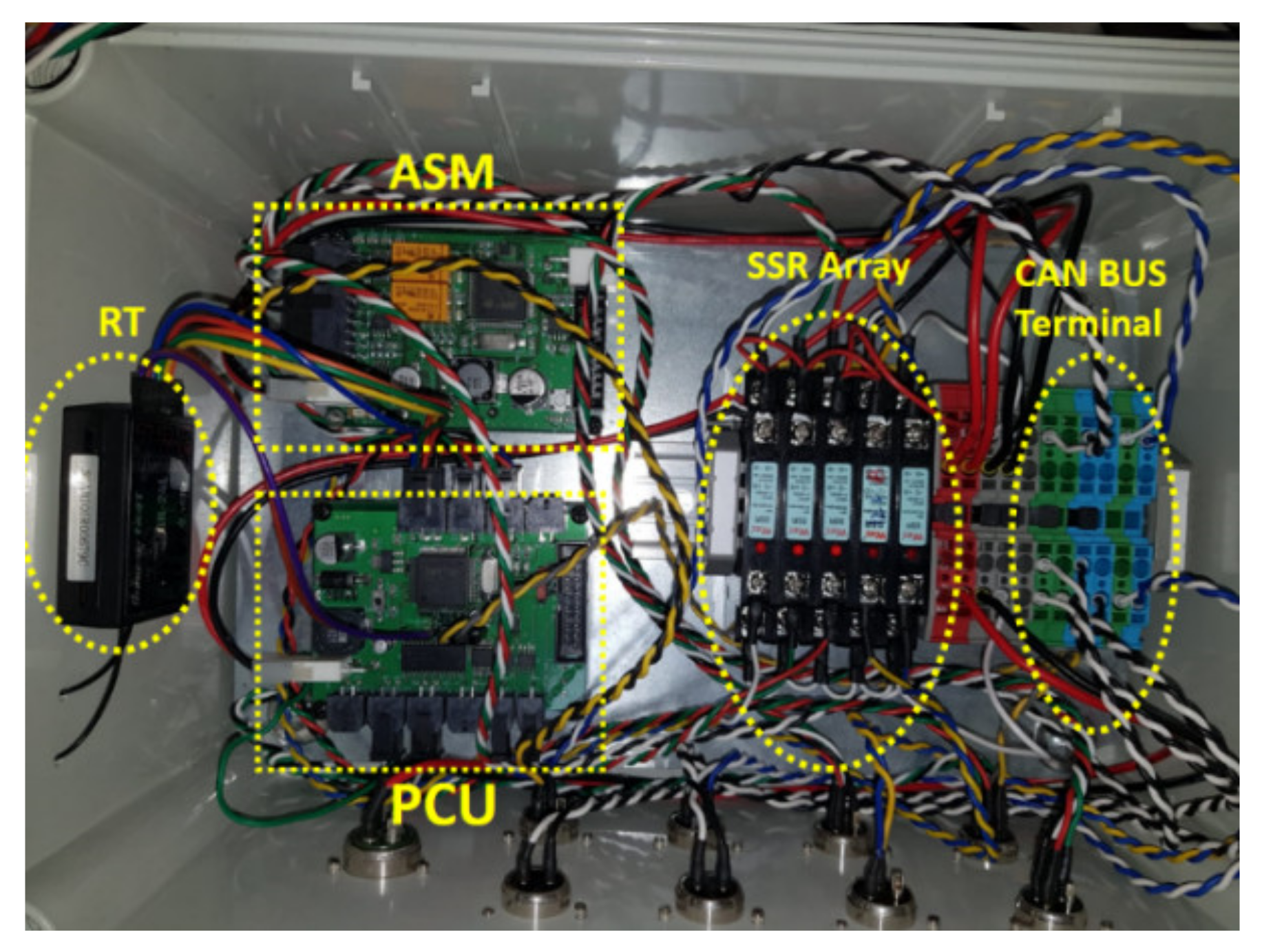
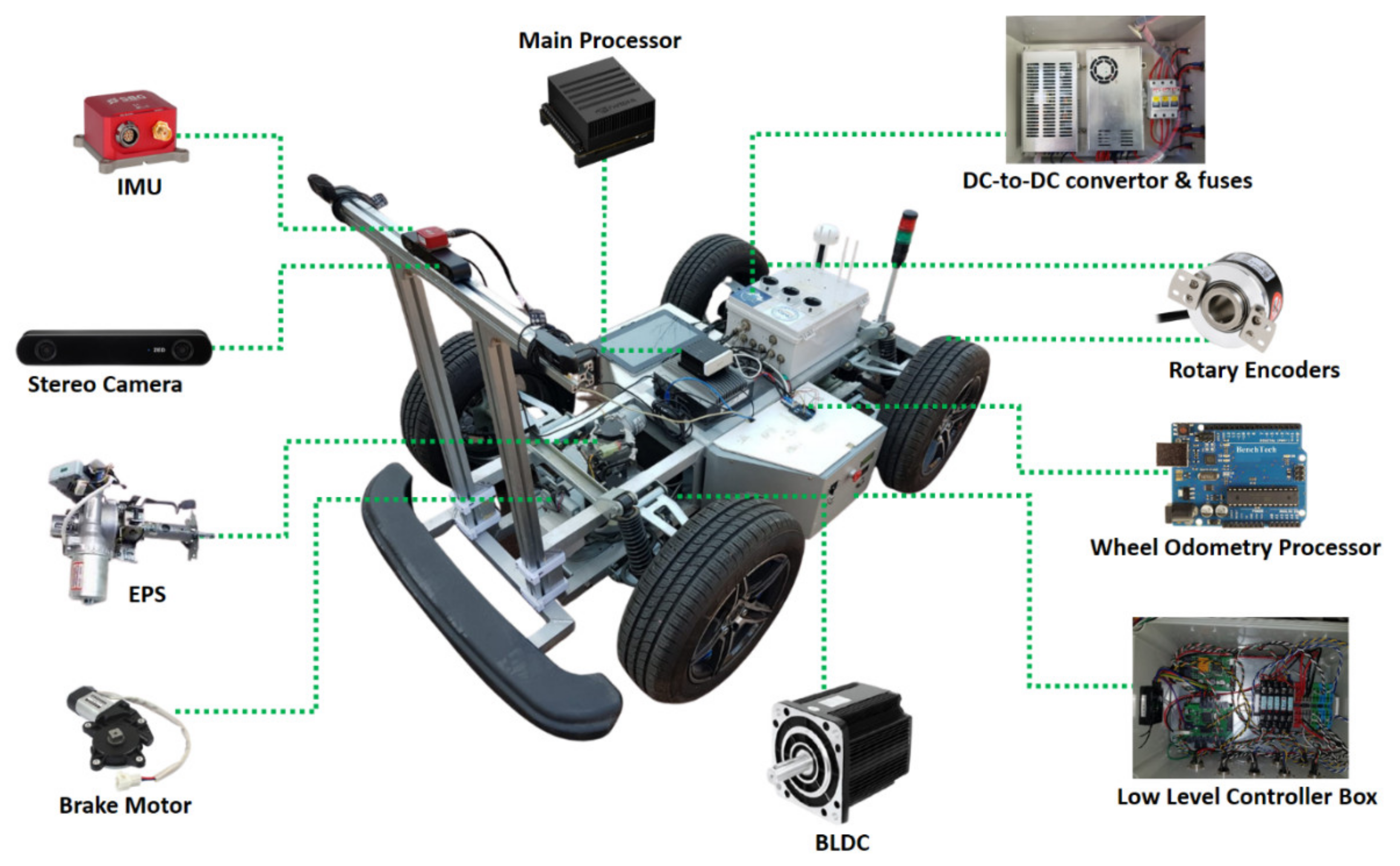
6. Hardware Architecture and Interfaces

System architecture and interfaces are shown in Figure 4. The system is comprised of two main parts, namely the high-level part and the low-level part (containing a low-level controller). The main processor is programmed to run the high-level controller algorithm, visual-inertial odometry, sensor fusion, and serial port communication with a low-level controller. The control commands are sent to the low-level controller that tries to control actuators including speed controller, brushless DC motor (BLDC), brake motor, and electronic power steering (EPS).

The main processor in this study is a Jetson AGX Xavier (NVIDIA Corporation, Santa Clara County, CA, USA). This is an embedded system-on-module (SOM) from the NVIDIA AGX Systems family. It is equipped with an octa-core NVIDIA Carmel ARMv8.2 CPU, 16 GB 256-bit LPDDRX with 137 GB/s, and other processing related to parallel processing, machine learning, and image processing. The processor runs the ROS on which the control algorithm, visual-inertial odometry algorithm, and sensor fusion algorithm are launched.

Table 2. Main processor specifications.

Hardware Unit	Specifications
GPU	512-core Volta GPU with tensor cores
CPU	8-core ARM v8.2 64-bit CPU, 8 MB L2 +4 MB L3
Memory	32 GB 256-bit LPDDR4xI137GB/s

shows the specifications of the main processor.

The main processor, and connections’ structure with other parts are shown in Figure 5. The incremental rotary encoders coupled with the wheels’ shafts provide data in the form of two square waves.

These raw data (from encoders) are sent to an Arduino Uno embedded processor board (Arduino Uno is an open-source microcontroller board employing an 8-bit AVR Microchip ATmega328P that is developed by Arduino). The processor board processes the square wave signals and generates the position and heading of the ground vehicle. An ELLIPSE2-N from SBG is employed as IMU. It contains an accelerometer with velocity random walk 100 (x,y) µg/$\sqrt{\mathrm{hz}}$ and 150 (z) µg/$\sqrt{\mathrm{hz}}$. The accelerometer bandwidth is 250 Hz while the sampling rate of the accelerometer is 3 kHz. The sensor also contains a gyroscope with an angular random walk of 0.16°/$\sqrt{\mathrm{hr}}$. The bandwidth of its gyroscope is 133 Hz, whereas the sampling rate is up to 10 kHz. It should be noted that the device is equipped with other aiding sensors, but in this study, we do not use them.

The device publishes inertial data with an update rate of up to 200 Hz. The IMU specifications are shown in

Table 3. IMU hardware specifications.

Accelerometer Parameters	Quantity	Gyroscopes Parameters	Quantity
Scale factor stability (%)	0.1	Scale factor stability (%)	0.05
Nonlinearity (% of FS)	0.2	Nonlinearity (% of FS)	0.05
One year bias stability (mg)	5	One year bias stability (°/s)	0.2
Velocity random walk (µg/$\sqrt{\mathrm{hz}}$)	100 (x,y)	Angular random walk (°/$\sqrt{\mathrm{hr}}$)	0.16
	150 (z)
In-run bias instability (µg)	20	In-run bias instability (°/hr)	8
Vibrating rectification error (mg/${\mathrm{g}}^2$)	7	Orthogonality	0.05
Bandwidth (Hz)	250	Bandwidth (Hz)	133
Sampling rate (kHz)	3	Sampling rate (kHz)	0.05

. The inertial measurement data are published via a topic in the ROS with the updated rate adjusted at 100 Hz.

A ZED stereo camera (StereoLabs, San Francisco, CA, USA) with resolution 2$\times \left(1920\times 1080\right)$ in 30 fps is employed to capture a stream of images. Its maximum field of view is 90° horizontal and 60° vertical. The camera image stream is received through its special package in the ROS.

Table 4. Stereo camera specifications.

Parameter	Specifications/Quantity
Output resolution	Side by side 2× (2208 × 1242) @ 15 fps
	2× (1920 × 1080) @ 30 fps 2× (1280 × 720) @ fps 2× (640 × 480) @ 100 fps
Output format	YUV 4:2:2
Field of view	Max. 110° (D)
Baseline	120 mm
Interface	USB 3.0
Sensor type	1/2.7″
Active array size	4 M pixels per sensor
Focal length	2.8 mm (0.11″)—f/2.0
Shutter	Electronic synchronized rolling shutter

shows the specifications of the stereo camera.

The low-level controller is comprised of two processor boards that are programmed to receive commands and control actuators. The actuators include the BLDC motor (with coupled gearbox), brake motor (responsible for controlling the flow of hydraulic oil from master brake pistons to caliper pistons), and electronic power steering (responsible for changing steering angle). Figure 6 shows the content of the low-level control box.

The platform control unit (PCU) is responsible for receiving control commands from the high-level controller via RS232 serial communication protocol. It also receives commands from a remote transceiver. The processor module establishes a Control Area Network Bus (CAN Bus) by which it can communicate with the automatic speed control module (ASM), brake motor driver, and electronic power steering (EPS). The BLDC motor is controlled by the ASM and PCU, while the brake and EPS are controlled through the PCU module. In Figure 6, RT stands for the remote transceiver. Solid state relays (SSR) play a role as electronic controlled switches. The final system configuration for the electric vehicle is depicted in Figure 7.

The electric vehicle employs a 3 kW BLDC motor with 3000 r/min that generates the needed torque. The rotational force is transferred to wheels via a gearbox and vehicle differential. The EPS communicates with the low-level controller through the CAN Bus. It is responsible for changing the steering angle. The brake motor driver also receives commands via the CAN Bus. The power supply box is equipped with several DC-to-DC converters that provide the proper voltage and current for each device. Figure 8 depicts the designed autonomous electric vehicle prototype.

7. Simulation and Real-Time Experimental Results from the Employed Localization Algorithm

In order to evaluate the performance of the VIO algorithm, the Malaga dataset [48] was used. At the second step, a real-time experiment with our designed electric vehicle prototype was performed to evaluate the performance of the integrated localization algorithm (VIO plus wheel odometry). The Malaga dataset was collected in different urban scenarios with a car equipped with a variety of different sensors including one stereo camera, an IMU, and laser sensors. This dataset provides different driving scenarios. In this study, a scenario named “short avenue loop closure” was used. Figure 9a shows the employed driving scenario. The size of the vehicle estimation trajectory was intentionally chosen to be bigger than that of the true trajectory, because we wanted to evaluate the ability of the filter for scale estimation. In this test, the ratio was defined to be three. Figure 9b shows the performance of the employed visual-inertial odometry in simulation as compared with the ground truth from a GPS in the dataset.

As it can be seen in Figure 9, although the scale of the VO trajectory was set to be three times bigger than the ground truth trajectory, the EKF was able to do scale estimation and provided correct estimation for VIO. In order to evaluate the performance of the proposed localization algorithm, an experiment using our designed electric vehicle was conducted. Figure 10 shows the result of the experiment that was conducted on the Kunsan National University campus.

From the result of the real-time experiment, it can be seen that the combination of the VIO and wheel odometry provides a far better estimation as compared with both the VO and VIO.

8. Simulation and Evaluation of the Employed Control Algorithm

The performance of the controller performing the trajectory-tracking maneuver was evaluated by defining a trajectory using (55)–(57) as follows:

$$X=10*e^{\cos \left(t\right)}$$

(55)

$$Y=15*e^{\sin \left(t\right)}$$

(56)

$${\Psi }_0=1.36\left(\mathrm{rad}\right)$$

(57)

where vectors of x and y coordinates in the trajectory plane are shown with X, Y. Heading at the starting point is shown with ${\Psi }_0$. Simulations were conducted using MATLAB and GAZEBO simulators. The CasADi package [49] was employed in order to solve the optimization problem. The package provides an open-source software framework for numerical optimization. The package is a general-purpose tool that can be used to model and solve optimization problems. The core of the package has been written in C++, but the creators made some interfaces for Python, MATLAB, and Octave. The package is widely using for academic purposes as well as in industrial applications in different fields, including optimal control, robotics control, and the aerospace industry. In this study, the optimizer used the IPOPT class inside the package. A primal-dual interior-point method was applied, which uses line search based on the filter method [50]. The software simulation architecture for evaluating the controller is shown in Figure 11.

Figure 12a depicts the desired trajectory and the performance of the trajectory tracking of the simulated vehicle. The vehicle heading angle error is shown in Figure 12b. The control inputs including velocity and steering angle are shown in Figure 13a,b, respectively. Lateral and longitudinal trajectory tracking performance (with respect to their occurrence time) are shown in Figure 14.

The simulation results in Figure 12 show that NMPC is able to control the car properly while tracking the trajectory. Simulation results, also, show that NMPC has optimized the controller effort during the simulation. In addition, the controller managed to steer the car towards the desired heading at the destination.

9. Real-Time Electric Vehicle Experimental Results

9.1. Trajectory Tracking

The proposed control and state estimation (the vehicle position and heading angle estimation) algorithms were implemented on our designed electric ground vehicle. A sinusoidal trajectory was defined as follows:

$$X_{trj}=1+t/10$$

(58)

$${\psi }_{des}=0$$

(59)

$$Y_{trj}=\sin \left(0.1*t\right)$$

(60)

We conducted a real-time trajectory tracking maneuver using our designed electric vehicle and the proposed system structure. Figure 15a,b show the trajectory tracking of the vehicle and the vehicle heading angle, respectively. Figure 16a shows vehicle linear velocity during the maneuver, while Figure 16b depicts vehicle trajectory tracking in the X coordinate (with respect to the occurrence time). It must be noted that the time shift in Figure 16b is the effect of the response delay of the system.

9.2. Path Following

The performance of the vehicle in performing path tracking was evaluated by conducting an experiment on the Kunsan university campus. Figure 17 shows the experimental result.

The controller is fed with waypoint data during the driving maneuver. Control inputs are depicted in Figure 18a. Figure 18b shows vehicle derivation from the desired path. The controller’s brake commands and changes in the vehicle steering angle, respectively, are shown in Figure 19a,b. Vehicle velocity and heading angle are shown in Figure 20.

10. Conclusions

In this study, we aimed to develop an autonomous electric vehicle for path tracking. We discussed both hardware and software design and implementation. Control and navigation algorithms were developed and implemented. The vehicle was able to perform path tracking maneuvers under environments in which the positioning signals from the Global Navigation Satellite System (GNSS) are not accessible. The proposed approach used a constrained input-output nonlinear model predictive controller (NMPC) for path tracking. The implemented localization algorithm guaranteed almost accurate position estimation under GNSS-denied environments.

The performances of the algorithms were evaluated using MATLAB and GAZEBO as simulators. In addition, the capability of the system was evaluated in real time by performing experiments using the designed vehicle. The simulation results and the real-time experiments confirm the capability of the designed vehicle for performing challenging path tracking under GNSS-denied environments.

References

1. Maghenem, M.; Loria, A.; Nuno, E.; Panteley, E. Distributed full-consensus control of nonholonomic vehicles under non-differentiable measurement delays. IEEE Control Syst. Lett. 2021, 5, 97–102. [Google Scholar] [CrossRef]
2. Zhao, P.; Chen, J.; Song, Y.; Tao, X.; Xu, T.; Mei, T. Design of a control system for an autonomous vehicle based on adaptive-PID. Int. J. Adv. Robot. Syst. 2012, 9, 44. [Google Scholar] [CrossRef]
3. Barzegar, A.; Piltan, F.; Vosoogh, M.; Mirshekaran, A.M.; Siahbazi, A. Design serial intelligent modified feedback linearization like controller with application to spherical motor. Int. J. Inf. Technol. Comput. Sci. 2014, 6, 72–83. [Google Scholar] [CrossRef] [Green Version]
4. Alouache, A.; Wu, Q. Genetic algorithms for trajectory tracking of mobile robot based on PID controller. In Proceedings of the 2018 IEEE 14th International Conference on Intelligent Computer Communication and Processing (ICCP), Cluj-Napoca, Romania, 6–8 September 2018. [Google Scholar]
5. Abdelhakim, G.; Abdelouahab, H. A new approach for controlling a trajectory tracking using intelligent methods. J. Electr. Eng. Technol. 2019, 14, 1347–1356. [Google Scholar] [CrossRef]
6. Thrun, S.; Montemerlo, M.; Dahlkamp, H.; Stavens, D.; Aron, A.; Diebel, J.; Fong, P.; Gale, J.; Halpenny, M.; Hoffmann, G.; et al. Stanley: The Robot That won the darpa grand challenge. In The 2005 DARPA Grand Challenge; Springer: Berlin/Heidelberg, Germany, 2007; Volume 36, p. 1. [Google Scholar]
7. Amer, N.H.; Hudha, K.; Zamzuri, H.; Aparow, V.R.; Abidin, A.F.Z.; Kadir, Z.A.; Murrad, M. Adaptive modified Stanley controller with fuzzy supervisory system for trajectory tracking of an autonomous armoured vehicle. Rob. Auton. Syst. 2018, 105, 94–111. [Google Scholar] [CrossRef]
8. Dominguez, S.; Ali, A.; Garcia, G.; Martinet, P. Comparison of lateral controllers for autonomous vehicle: Experimental results. In Proceedings of the 2016 IEEE 19th International Conference on Intelligent Transportation Systems (ITSC), Rio de Janeiro, Brazil, 1–4 November 2016. [Google Scholar]
9. Morales, J.; Martínez, J.L.; Martínez, M.A.; Mandow, A. Pure-pursuit reactive path tracking for nonholonomic mobile robots with a 2D laser scanner. EURASIP J. Adv. Signal Process. 2009. [Google Scholar] [CrossRef] [Green Version]
10. Pure Pursuit Controller-MATLAB & Simulink. Available online: https://www.mathworks.com/help/robotics/ug/pure-pursuit-controller.html (accessed on 30 January 2021).
11. Mobarez, E.N.; Sarhan, A.; Ashry, M.M. Comparative robustness study of multivariable controller of fixed wing Ultrastick25-e UAV. In Proceedings of the 2018 14th International Computer Engineering Conference (ICENCO), Giza, Egypt, 29–30 December 2018. [Google Scholar]
12. Norouzi, A.; Kazemi, R.; Azadi, S. Vehicle lateral control in the presence of uncertainty for lane change maneuver using adaptive sliding mode control with fuzzy boundary layer. Proc. Inst. Mech. Eng. Part I J. Syst. Control Eng. 2018, 232, 12–28. [Google Scholar] [CrossRef]
13. National Aeronaut Administration (Nasa). An Improved Lateral Control Wheel Steering Law for The Transport Systems Research Vehicle (TSRV); Createspace Independent Publishing Platform: North Charleston, SC, USA, 2018; ISBN 9781722072544. [Google Scholar]
14. Vivek, K.; Ambalal Sheta, M.; Gumtapure, V. A comparative study of Stanley, LQR and MPC controllers for path tracking application (ADAS/AD). In Proceedings of the 2019 IEEE International Conference on Intelligent Systems and Green Technology (ICISGT), Visakhapatnam, India, 29–30 June 2019. [Google Scholar]
15. Camacho, E.F.; Bordons Alba, C. Model Predictive Control, 2nd ed.; Springer: London, UK, 2007; ISBN 9780857293985. [Google Scholar]
16. Findeisen, R.; Allgöwer, F. An Introduction to Nonlinear Model Predictive Control; Technische Universiteit Eindhoven Veldhoven: Eindhoven, The Netherlands, 2002; Volume 11, pp. 119–141. [Google Scholar]
17. Canale, M.; Fagiano, L. Vehicle yaw control using a fast NMPC approach. In Proceedings of the 2008 47th IEEE Conference on Decision and Control, Cancun, Mexico, 9–11 December 2008. [Google Scholar]
18. Kong, J.; Pfeiffer, M.; Schildbach, G.; Borrelli, F. Kinematic and dynamic vehicle models for autonomous driving control design. In Proceedings of the 2015 IEEE Intelligent Vehicles Symposium (IV), Seoul, South Korea, 28 June–1 July 2015. [Google Scholar]
19. Menhour, L.; d’Andrea-Novel, B.; Boussard, C.; Fliess, M.; Mounier, H. Algebraic nonlinear estimation and flatness-based lateral/longitudinal control for automotive vehicles. In Proceedings of the 2011 14th International IEEE Conference on Intelligent Transportation Systems (ITSC), Washington, DC, USA, 5–7 October 2011. [Google Scholar]
20. Mur-Artal, R.; Montiel, J.M.M.; Tardos, J.D. ORB-SLAM: A versatile and accurate monocular SLAM system. IEEE Trans. Robot. 2015, 31, 1147–1163. [Google Scholar] [CrossRef] [Green Version]
21. Mur-Artal, R.; Tardos, J.D. ORB-SLAM2: An open-source SLAM system for monocular, stereo and RGB-D cameras. IEEE Trans. Robot. 2017, 33, 1255–1262. [Google Scholar] [CrossRef] [Green Version]
22. Rublee, E.; Rabaud, V.; Konolige, K.; Bradski, G. ORB: An efficient alternative to SIFT or SURF. In Proceedings of the 2011 International Conference on Computer Vision, Barcelona, Spain, 6–13 November 2011. [Google Scholar]
23. Engel, J.; Schöps, T.; Cremers, D. LSD-SLAM: Large-scale direct monocular SLAM. In European Conference on Computer Vision, Proceedings of the ECCV 2014: Computer Vision—ECCV 2014, Zurich, Switzerland, 6–12 September 2014; Springer International Publishing: Cham, Switzerland, 2014; pp. 834–849. ISBN 9783319106045. [Google Scholar]
24. Goncalves, T.; Comport, A.I. Real-time direct tracking of color images in the presence of illumination variation. In Proceedings of the 2011 IEEE International Conference on Robotics and Automation, Shanghai, China, 9–13 May 2011. [Google Scholar]
25. Forster, C.; Pizzoli, M.; Scaramuzza, D. SVO: Fast semi-direct monocular visual odometry. In Proceedings of the 2014 IEEE International Conference on Robotics and Automation (ICRA), Hong Kong, China, 31 May–5 June 2014. [Google Scholar]
26. Krombach, N.; Droeschel, D.; Behnke, S. Combining feature-based and direct methods for semi-dense real-time stereo visual odometry. In Intelligent Autonomous Systems 14; Springer International Publishing: Cham, Switzerland, 2017; pp. 855–868. ISBN 9783319480350. [Google Scholar]
27. Fanani, N. Predictive Monocular Odometry Using Propagation-Based Tracking; Goethe-Universität Frankfurt: Johann Wolfgang, Germany, 2018. [Google Scholar]
28. Oskiper, T.; Zhu, Z.; Samarasekera, S.; Kumar, R. Visual odometry system using multiple stereo cameras and inertial measurement unit. In Proceedings of the 2007 IEEE Conference on Computer Vision and Pattern Recognition, Minneapolis, MN, USA, 17–22 June 2007. [Google Scholar]
29. Sensing and Control for Autonomous Vehicles: Applications to Land, Water and Air Vehicles, 1st ed.; Fossen, T.I.; Pettersen, K.Y.; Nijmeijer, H. (Eds.) Springer International Publishing: Cham, Switzerland, 2017; ISBN 9783319553726. [Google Scholar]
30. Jimenez, A.R.; Seco, F.; Prieto, J.C.; Guevara, J. Indoor pedestrian navigation using an INS/EKF framework for yaw drift reduction and a foot-mounted IMU. In Proceedings of the 2010 7th Workshop on Positioning, Navigation and Communication, Dresden, Germany, 11–12 March 2010. [Google Scholar]
31. Weiss, S.; Siegwart, R. Real-time metric state estimation for modular vision-inertial systems. In Proceedings of the 2011 IEEE International Conference on Robotics and Automation, Shanghai, China, 9–13 May 2011. [Google Scholar]
32. Leutenegger, S.; Lynen, S.; Bosse, M.; Siegwart, R.; Furgale, P. Keyframe-based visual–inertial odometry using nonlinear optimization. Int. J. Robot. Res. 2015, 34, 314–334. [Google Scholar] [CrossRef] [Green Version]
33. Yang, Z.; Shen, S. Monocular visual-inertial state estimation with online initialization and camera–IMU extrinsic calibration. IEEE Trans. Autom. Sci. Eng. 2017, 14, 39–51. [Google Scholar] [CrossRef]
34. Usenko, V.; Engel, J.; Stuckler, J.; Cremers, D. Direct visual-inertial odometry with stereo cameras. In Proceedings of the 2016 IEEE International Conference on Robotics and Automation (ICRA), Stockholm, Sweden, 16–21 May 2016. [Google Scholar]
35. Yang, G.; Zhao, L.; Mao, J.; Liu, X. Optimization-based, simplified stereo visual-inertial odometry with high-accuracy initialization. IEEE Access 2019, 7, 39054–39068. [Google Scholar] [CrossRef]
36. Mourikis, A.I.; Roumeliotis, S.I. A multi-state constraint Kalman filter for vision-aided inertial navigation. In Proceedings of the 2007 IEEE International Conference on Robotics and Automation, Roma, Italy, 10–14 April 2007. [Google Scholar]
37. Bloesch, M.; Omari, S.; Hutter, M.; Siegwart, R. Robust visual inertial odometry using a direct EKF-based approach. In Proceedings of the 2015 IEEE/RSJ International Conference on Intelligent Robots and Systems (IROS), Hamburg, Germany, 28 September–2 October 2015. [Google Scholar]
38. Tsotsos, K.; Chiuso, A.; Soatto, S. Robust inference for visual-inertial sensor fusion. In Proceedings of the 2015 IEEE International Conference on Robotics and Automation (ICRA), Seattle, WA, USA, 26–30 May 2015. [Google Scholar]
39. Kelly, J.; Sukhatme, G.S. Visual-inertial sensor fusion: Localization, mapping and sensor-to-sensor self-calibration. Int. J. Robot. Res. 2011, 30, 56–79. [Google Scholar] [CrossRef] [Green Version]
40. Sun, K.; Mohta, K.; Pfrommer, B.; Watterson, M.; Liu, S.; Mulgaonkar, Y.; Taylor, C.J.; Kumar, V. Robust stereo visual inertial odometry for fast autonomous flight. arXiv 2017, arXiv:1712.00036. [Google Scholar] [CrossRef] [Green Version]
41. Trajković, M.; Hedley, M. Fast corner detection. Image Vis. Comput. 1998, 16, 75–87. [Google Scholar] [CrossRef]
42. Barzegar, A.; Doukhi, O.; Lee, D.-J.; Jo, Y.-H. Nonlinear Model Predictive Control for Self-Driving cars Trajectory Tracking in GNSS-denied environments. In Proceedings of the 2020 20th International Conference on Control, Automation and Systems (ICCAS), Busan-City, Korea, 13–16 October 2020. [Google Scholar]
43. Huang, G.P.; Mourikis, A.I.; Roumeliotis, S.I. Observability-based rules for designing consistent EKF SLAM estimators. Int. J. Robot. Res. 2010, 29, 502–528. [Google Scholar] [CrossRef] [Green Version]
44. Hesch, J.A.; Kottas, D.G.; Bowman, S.L.; Roumeliotis, S.I. Observability-constrained vision-aided inertial navigation. Univ. Minn. Dep. Comput. Sci. Eng. MARS Lab. Tech. Rep. 2012, 1, 6. [Google Scholar]
45. Castellanos, J.A.; Martinez-Cantin, R.; Tardós, J.D.; Neira, J. Robocentric map joining: Improving the consistency of EKF-SLAM. Rob. Auton. Syst. 2007, 55, 21–29. [Google Scholar] [CrossRef] [Green Version]
46. Moore, T.; Stouch, D. A generalized extended Kalman filter implementation for the robot operating system. In Intelligent Autonomous Systems 13; Springer International Publishing: Cham, Switzerland, 2016; pp. 335–348. ISBN 9783319083377. [Google Scholar]
47. Matute, J.A.; Marcano, M.; Diaz, S.; Perez, J. Experimental validation of a kinematic bicycle model predictive control with lateral acceleration consideration. IFAC Pap. OnLine 2019, 52, 289–294. [Google Scholar] [CrossRef]
48. The Málaga Stereo and Laser Urban Data Set. Available online: https://www.mrpt.org/MalagaUrbanDataset (accessed on 22 February 2021).
49. Andersson, J.A.E.; Gillis, J.; Horn, G.; Rawlings, J.B.; Diehl, M. CasADi: A software framework for nonlinear optimization and optimal control. Math. Program. Comput. 2019, 11, 1–36. [Google Scholar] [CrossRef]
50. Wächter, A.; Biegler, L.T. On the implementation of an interior-point filter line-search algorithm for large-scale nonlinear programming. Math. Program. 2006, 106, 25–57. [Google Scholar] [CrossRef]
Figure 1. Controller and localization system architecture.
Applsci 11 03688 g001
Figure 2. Wheel odometry model.
Applsci 11 03688 g002
Figure 3. Rear axle bicycle model.
Applsci 11 03688 g003
Figure 4. System architecture and interfaces.
Applsci 11 03688 g004
Figure 5. Main processor and its connection to other parts.
Applsci 11 03688 g005
Figure 6. Platform control unit and low-level controller.
Applsci 11 03688 g006
Figure 7. Electric vehicle system configuration.
Applsci 11 03688 g007
Figure 8. The prototype of the electric vehicle.
Applsci 11 03688 g008
Figure 9. Driving scenario from Malaga and localization algorithm simulation result with the Malaga dataset. (a) Short avenue loop closure driving scenario dataset from Malaga; (b) performance of employed visual-inertial odometry in simulation with the Malaga dataset.
Applsci 11 03688 g009
Figure 10. Real-time experiments with the proposed localization algorithm.
Applsci 11 03688 g010
Figure 11. Software simulation architecture for evaluating the vehicle controller.
Applsci 11 03688 g011
Figure 12. Results of simulation for trajectory-tracking and heading error. (a) Desired trajectory Vs the trajectory made by the simulated vehicle; (b) heading angle error.
Applsci 11 03688 g012
Figure 13. Control inputs. (a) Velocity; (b) Steering.
Applsci 11 03688 g013
Figure 14. Lateral and longitudinal trajectory tracking of the vehicle with respect to their occurrence time (note that the time shift in the figures is the effect of the propagation delay of the system). (a) Longitudinal trajectory with respect to time; (b) lateral trajectory with respect to time.
Applsci 11 03688 g014
Figure 15. Heading and trajectory. (a) Trajectory tracked by the vehicle; (b) heading of the electric vehicle.
Applsci 11 03688 g015
Figure 16. Velocity and the performance of the trajectory tracking of the vehicle in X coordinate with respect to time. (a) Vehicle velocity; (b) trajectory tracking of the vehicle (in X coordinate) with respect to time (note that the time delay in the figure is the propagation delay of the system that caused a time shift between graphs).
Applsci 11 03688 g016
Figure 17. Result of path-following maneuver by the vehicle.
Applsci 11 03688 g017
Figure 18. Vehicle derivation from desired path and control inputs. (a) Control inputs; (b) vehicle derivation from desired path during maneuver.
Applsci 11 03688 g018
Figure 19. Brake commands and changes in vehicle steering angle: (a) brake commands; (b) changes in vehicle steering angle.
Applsci 11 03688 g019
Figure 20. Vehicle velocity and heading angle. (a) Vehicle velocity; (b) vehicle heading.
Applsci 11 03688 g020