Employing Finite Element Analysis and Robust Control Concepts in Mechatronic System Design-Flexible Manipulator Case Study

Abstract

The paper deals with development of a methodology for mechatronic system design using state-of-the-art model-based system engineering methods. A simple flexible robotic arm is considered as a benchmark problem for the evaluation of various techniques used in the phases of modelling, analysis, control system design, validation, and implementation. The flexible nature of the mechanical structure introduces inherently oscillatory dynamics in the target bandwidth range, which complicates all the above-mentioned design steps. This paper demonstrates the process of deriving a complex nonlinear model of the flexible arm setup. An initial idea about the plant dynamics is acquired from analytical modelling using the Euler–Bernoulli beam theory. A more thorough understanding is subsequently acquired from finite element analysis. Linearisation and order reduction are the next steps necessary for the derivation of a simplified control-relevant model. A time-dependent variable parameter of load mass position is considered and a robust controller is subsequently designed in order to fulfil certain performance criteria for all the admissible plant configurations. This is performed using a recent H-infinity loop shaping method for fixed structure controller design. The results are validated by means of a physical plant, comparing the experimental data with the model predictions.

1. Introduction

Mathematical modelling has become the cornerstone of many technical disciplines. Models generally allow us to gain insight, answers, and guidance when analysing and predicting the behaviour of complex systems. Model-based engineering methods also provide essential tools in the field of mechatronics. Derivation of relevant models enables the optimisation of machine design before physical prototype assembly. This may help to avoid costly build-and-test cycles, speeding up the whole development process considerably. A high-fidelity model is a necessary prerequisite for employing modern control engineering methods and algorithms. It can be said that the achievable performance of a motion system is directly proportional to the predictive and explanatory power of the model used for the controller synthesis. On the other hand, an excessively complex model, albeit well suited for numerical simulations and predictions, may turn out to be useless for the process of control algorithms design. High-order nonlinear models are generally incompatible with well-established and generally applicable control design methods working mainly in the linear domain. Therefore, a general rule of thumb is to use a control-relevant model that is as simple as possible while capturing the significant features of the physical plant’s dynamics essential for achieving formulated design requirements.

Mathematical models of dynamic mechanical systems can be generally derived in two distinct ways. First-principles (or physics-based, white-box) approaches use all the available prior knowledge about the subject of study for the derivation of the equations of motion. This involves information about the system structure and geometry, basic laws of physics, mechanics, and other domains necessary to cover all the aspects of the system behaviour. The model parameters usually have an exact physical meaning and are closely related to the properties of the system under study. On the other hand, a data-driven (or black-box) approach uses quite a limited amount of a priori knowledge regarding the system and tries to deduce its dynamical properties indirectly by observing available input and output variables [1]. The model parameters often do not have a clear physical interpretation. They result from the specifically used data processing method and chosen model structure. The white-box method usually requires extensive knowledge about the physical system that may not be available in practice. Considerable effort is often required for the model derivation. The advantage is that the model may be inferred without having to construct and assemble a physical device. Therefore, such models may provide valuable insight when designing new systems that do not physically exist yet. On the other hand, the black-box approach is relatively simple to use when employing well-established methods available in the field of system identification [1,2,3]. Much less prior knowledge about the system is required, and high-fidelity models can be acquired from experimental data with less effort. However, back-box modelling typically depends on an extensive amount of the input-output data which have to be obtained from the experiments with the physical plant. A combination of both approaches can be used forming a grey-box modelling concept. In this case, the model properties and its structure are at least partially known in advance and particular parameters are derived from experimental data.

The role of the model is being emphasised and changed at the same time significantly with the introduction of the Digital Twin concept [4,5,6,7]. There is a fundamental shift in the understanding of what the model represents and how it can interact with its physical counterpart in the form of a device or machine to be designed and built. Formerly a static abstraction of the reality used in the early stages of the development cycle is being gradually transformed into a dynamic object living a parallel life with the physical plant and continuously updating its inner states, structure, or parameters. The goal is to improve the fidelity of the model and obtain the best achievable digital copy of the real system. This allows enhancing the predictive quality of the model to bring new possibilities in terms of monitoring, predictive or reactive maintenance and diagnostics, and accurate model-based control design. The Digital Twin can be instanced, representing a particular piece of hardware to capture specific deviations from the idealised expected behaviour, e.g., due to production variations or increasing wear during machine operation. It can be involved in all stages of a product or system’s life cycle, including the design, the production, and the operation. The key difference between Digital Twin modelling and conventional numerical models is that besides the design of the product or system, the Digital Twin model incorporates all applicable data for each instance of the product or system separately. Among others, the Digital Twin model can include data considering the production, tests and measurements, operation history, and sensor data in its predictions and adapts itself continuously by synchronisation with the latest available data. Furthermore, physics-based modelling techniques such as the finite element method (FEM) can be incorporated in a Digital Twin, by continuously synchronising history and model parameters with measurement, sensor, and history data of an instance of the product.

Finite element method (FEM) belongs to the class of widely applied physics-based modelling approaches. Using the FEM models for studying and analysing underlying phenomena is often designated as Finite element analysis (FEA). Many software packages that implement the FEM are available, both commercial (Abaqus, OOFELIE, Ansys and Nastran for example) and free (Elmer, Code-Aster and CalculiX for example). Books about the theory of the FEM include [8,9]. The advantage of an FE model is that the entire mechanism response is available, not just the few lumped parameters. This enables the use of the model as a Digital Twin. It may be used to optimise sensor placement, detect damage, predict fatigue, schedule maintenance, gather data to improve redesign, and so on. However, having a high fidelity FE model is not enough. The model is not useful as a Digital Twin if evaluating it costs hours or even days. It must be much faster. This is where model reduction comes in. This paper presents an example of how a FE model can be reduced. This example is related to mechatronic design, but it could be expanded to cover more Digital Twin functionalities.

The main motivation of our research was to review state-of-the-art techniques, methods, algorithms, and software tools available in the field of modelling, identification, and control and connect them in a suitable workflow applicable for designing high-fidelity motion systems. While there are many research papers dealing with the individual parts of the design process separately, we felt that a unifying view allowing us to bridge different fields of mechatronics will be beneficial for researchers and engineers working in the respective domains. Special attention is paid to the derivation of control-relevant models applicable to generic robust control methods. Subsequent steps of physical modelling using both analytical and FEM approaches, model linearization, order reduction, and model-based controller synthesis are demonstrated on a chosen benchmark problem dealing with flexible manipulator arm control. The predictive capability of the developed models is analysed by comparing their outputs with the experimentally acquired data. Suggestions on how to improve model fidelity based on the experiments are given. The ultimate goal is to assess the applicability of the physics-based modelling in giving accurate predictions for the design of the motion control system.

The paper is organised as follows. Section 2 introduces a flexible arm motion setup used to validate proposed modelling and robust control design methods. Basic principles of analytical modelling of flexible mechanisms using Euler–Bernoulli beam theory, geometrical modelling using Finite element analysis, frequency domain experimental identification, and robust fixed-structure controller design method are provided as well. Section 3 deals with application of the proposed methods on our flexible arm manipulator problem. Analytical and geometrical models are derived and compared with experimentally acquired data. The observations are used to improve fidelity of the models. On the other hand, analysis of the geometric model reveals potential drawbacks in actual machine design that are corrected. This forms a model–measurement loop leading to improvement in both model predictions and actual machine operation. A robust controller is derived for a whole set of plant models coming from assumed parametric uncertainty in machine geometric configuration. Closed-loop performance and models fidelity are experimentally validated using the flexible arm setup. Final remarks concluding our findings and open topics for a future research are given in Section 4 and Section 5, respectively.

2. Materials and Methods

2.1. Flexible Arm Benchmark Problem

A flexible arm motion setup from Figure 1 is used to demonstrate the applicability of the presented methods in various stages of mechatronic system design. The motion system consists of an electrical drive (590 W permanent magnets synchronous motor driven by a servo amplifier), flexible coupling, bearing housing, inertia flywheel, and removable flexible arm with adjustable load mass. One degree of freedom allows the arm to rotate freely around the vertical axis. Details of the drive and arm assembly are shown in Figure 2.

Albeit simple, its mechanical structure allows emulating various practical motion control problems encountered in industrial applications. Some essential features are given below:

• Distributed parameter system exhibiting oscillatory dynamics with a possible introduction of multiple resonance modes, nonlinear friction effects and parametric uncertainty (e.g., load mass and/or position)
• A diverse range of dynamic response achievable by adjusting/interchanging the attached load
• Both actuator and load-side feedback possible through the optical encoder at the motor shaft and MEMS accelerometers attached to the load
• Industrial grade drive system with servo amplifier implementing field-oriented control loop
• EtherCAT communication with 5 kHz update rate to the B&R Automation PC master controller
• Hard real-time Linux-based software environment with REXYGEN control system [10]

A wide range of dynamic behaviour can be achieved in order to emphasise specific desired characteristics of a represented motion system. Typical scenarios include, for example, a rigid body system, flexible load with one or several dominant bending modes, friction-dominant system, unbalanced rotor system etc. The setup proved to be a valuable benchmark problem for the evaluation of various methods from the field of mechatronics, including modelling, identification, and feedback control design [11,12,13,14].

Table 1. Drive, sensors and control system parameters.

Main actuator	TG Drives TGN3-0480-5-320
$n_n$: Rated speed	1200 rpm
$n_{max}$: Maximum speed	12,000 rpm
$U_{DC}$: DC Bus Voltage	320 V
$M_n$: Rated torque	4.7 Nm
$M_{max}$: Peak torque	14.4 Nm
$P_n$: Rated power	590 W
$J_m$: Rotor inertia	1.5 $\mathrm{kg}.{\mathrm{cm}}^2$
Motor-load coupling	Direct connection to bearing house via flexible coupling
Servoamplifier	TG Drives TGZ-320
$P_o$: Operating power	1600 W for S1 operation
$I_{cmax}$: Maximum continuous current	5 A
$I_{max}$: Maximum output current (5s)	10 A
Current control loop	Field Oriented Control with position feedback
Fieldbus	EtherCAT, 5 kHz update rate
Sensors	Motor and load side feedback
Motor position/velocity	Integrated optical encoder, 20 bits/rev resolution, Hiperface DSL interface
Arm acceleration	Kistler piezo-ceramic MEMS accerlerometers, ±50 g range
Supervisory control system
HW platform	B&R Automation PC 910
Operating system	Debian Linux with RT patch
Real-time SW environment	REXYGEN control system

summarises the important specifications of the employed actuator, sensors, and control instrumentation.

Table 2. Mechanical parameters of the flexible arm motion stage.

L: Length of the arm	0.235 $\mathbf{m}$
$\rho$: Density of the arm material	8030 $\mathrm{kg} {\mathrm{m}}^{-3}$
E: Young’s modulus of the material	190,295,301,291.7 N m−2
I: Second moment of the link area	6.5182 × 10−11 ${\mathrm{m}}^4$
S: Cross section area	8.9274 × 10−5 ${\mathrm{m}}^2$
$m_i$: Mass per one element	0.7169 kg m−1
$m_p$: Mass of the payload	1.049 $\mathrm{kg}$
$J_h$: Moment inertia of the hub	0.0024 $\mathrm{kg} {\mathrm{m}}^2$

provides mechanical parameters of the flexible arm motion system under study. The purpose of the installed sensory system is twofold. The high-fidelity motor side optical sensor is used for precise control of the actuator serving for its electronic commutation using field-oriented control algorithm as well as for supervisory velocity and position loops. Removable accelerometers can be installed at different positions of the flexible arm in order to evaluate the load-side dynamic responses. They were used to validate both open- and closed-loop predictions provided by developed mathematical models in our actual application. This additional load-side feedback may also serve for employing advanced control schemes allowing to improve overall performance of the motion system, see, e.g., [14]. However, this topic is out of scope of this study, which focuses on the modelling, identification, and control aspects using conventional control topologies available in current industrial-grade automation equipment.

For the case study presented in this paper, we focused on the load configuration producing a dynamics with three dominant bending modes. This situation is often encountered in robotic applications, where the oscillatory dynamics results from the mechanical compliance of either gearing, the robot arm itself, or due to combination of flexibility of both components [15,16].

Proper mechanical design followed by optimisation of the control layer is a key step for delivering new generation of robotic products fulfilling stringent performance and safety requirements. The safety aspect becomes crucial in the applications of robots that interact directly with humans, such as social robots or collaborative robots in factories. The mechanical flexibility is often introduced deliberately as a safety feature to minimise impact forces during unwanted collisions. Special attention is required during modelling, identification, and control design to achieve optimal performance of the motion system in terms of fast reference tracking and suppression of unwanted transient or residual oscillations. Well-designed bottom layers of control system enable employing advanced supervisory algorithms for motion planning and control [17,18]. For example, recent advances in neurobiology reveal new possibilities of connecting human brain in the loop for direct robot commanding [19]. It is clear that high-fidelity models of such mechatronic systems are required to provide reliable predictions of their behaviour.

In our paper, state-of-the-art methods based on analytical and geometrical approaches are used to derive a mathematical model of flexible arm manipulator. Experiments with the real plant follow to evaluate the validity of the physics-based models. Possibilities of enhancing physical models’ fidelity using experimental data are discussed, proposing a workflow which combines the best of the two worlds of white-box and black-box modelling. A robust control scenario is formulated by assuming a parametric uncertainty in the mechanical structure of the system aiming at delivery of a fixed-structure controller achieving specified closed-loop performance for all the possible plant variations.

2.2. Analytical Modelling of Flexible Mechanisms Using Euler–Bernoulli Beam Theory

For various kind of mechatronic systems, we are able to derive the system of ordinary/partial differential or differential-algebraic equations from the mathematical-physical principles. However, for control design purposes, the aim is to obtain a simplified model allowing to get a better insight into the dynamics. Therefore, some compromises have to be made. Basically, some primary knowledge about the dominant modes distribution is useful to also help design the controller structure and to find suitable controller parameters. The Lagrange–Euler method [20] and the finite element method, together with the Euler–Bernoulli beam theory under specific assumptions [21,22], were followed to derive the dynamic model of the studied flexible arm.

In general, flexible beams are handled as the systems with distributed elasticity [23,24], which can be described by the partial differential equations:

$$\frac{{\partial }^2}{\partial x^2}\left(EI\frac{{\partial }^{2}u(x,t)}{\partial x^2}\right)+\mu \frac{{\partial }^{2}u(x,t)}{\partial t^2}=f(x,t),$$

(1)

$$u(x,t)\approx \sum _{i=1}^n{N}_i\left(x\right)q_i\left(t\right),$$

(2)

where n is the number of considered finite elements with each of the same length l; therefore, the beam length can be denoted as $L=l\ast n$. On each element, two nodes are introduced. This leads to four state variables dedicated to each element. The state vector of the ith element can be written as ${\left[\begin{array}{cccc}{q}_{2i-1}\left(t\right)& q_{2i}\left(t\right)& q_{2i+1}\left(t\right)& q_{2i+2}\left(t\right)\end{array}\right]}^T$, where $q_{2i-1}$ is the displacement of the node $i-1$, $q_{2i+1}$ denotes the displacement of the neighbouring node i, $q_{2i}$ is the angle in the node $i-1$, and $q_{2i+2}$ is the angle in the node i.

The corresponding shape functions $N_i\left(x\right)$ are chosen as the cubic Hermitian functions [24] to meet the requirements following from Euler–Bernoulli beam theory ([21,23,25,26]) regarding continuity between elements, continuity on borders, and completeness [23,24]. To express the suitable coefficients $N_i\left(x\right)$ and to establish the state variables, let us present the auxiliary function $w_i(x,t)$,

$$w^i(x,t)={\alpha }_1+{\alpha }_{2}x+{\alpha }_3{x}^2+{\alpha }_4{x}^3,$$

(3)

where αs are the auxiliary time-variant functions. The boundary conditions are set to $w_1^i\left(t\right)\triangleq w^i(0,t)={\alpha }_1$, $w_2^i\triangleq w^i(l,t)={\alpha }_1+{\alpha }_{2}l+{\alpha }_3{l}^2+{\alpha }_4{l}^3$, ${\theta }_1^i\left(t\right)\triangleq \frac{\partial w^i(x,t)}{\partial x}(0,t)={\alpha }_2$, ${\theta }_2^i\left(t\right)\triangleq \frac{\partial w^i(x,t)}{\partial x}\left(l\right)={\alpha }_2+2{\alpha }_{3}l+3{\alpha }_4{l}^2$. These given requirements are gathered as

$$\left[\begin{array}{c}{w}_1^i\\ {\theta }_1^i\\ w_2^i\\ {\theta }_2^i\end{array}\right]=\left[\begin{array}{cccc}\hfill 1& \hfill 0& \hfill 0& \hfill 0\\ \hfill 0& \hfill 1& \hfill 0& \hfill 0\\ \hfill 1& \hfill l& \hfill l^2& \hfill l^3\\ \hfill 0& \hfill 1& \hfill 2l& \hfill 3l^2\end{array}\right]\left[\begin{array}{c}{\alpha }_1\\ {\alpha }_2\\ {\alpha }_3\\ {\alpha }_4\end{array}\right].$$

(4)

By expressing $\alpha$’s from (4) and substituting into (3), we obtain

$$w^i(x,t)=\left[\begin{array}{cccc}1\hfill & x\hfill & x^2\hfill & x^3\hfill \end{array}\right]\left[\begin{array}{cccc}\hfill 1& \hfill 0& \hfill 0& \hfill 0\\ \hfill 0& \hfill 1& \hfill 0& \hfill 0\\ \hfill -\frac{3}{l^2}& \hfill -\frac{2}{l}& \hfill \frac{3}{l^2}& \hfill -\frac{1}{l}\\ \hfill \frac{2}{l^3}& \hfill \frac{1}{l^2}& \hfill -\frac{2}{l^3}& \hfill \frac{1}{l^2}\end{array}\right]\left[\begin{array}{c}{w}_1^i\\ {\theta }_1^i\\ w_2^i\\ {\theta }_2^i\end{array}\right].$$

(5)

This formula leads to the desired separated time/space interpolation, $w^i(x,t)=N^i\left(x\right)q^i\left(t\right)$, where

$$N^i\left(x\right)=[1-\frac{3}{l^2}{x}^2+\frac{2}{l^3}{x}^3 x-\frac{2}{l}{x}^2+\frac{1}{l^2}{x}^3 \frac{3}{l^2}{x}^2-\frac{2}{l^3}{x}^3 -\frac{1}{l}{x}^2+\frac{1}{l^2}{x}^3],q^i\left(t\right)=\left[\begin{array}{c}{w}_1^i\left(t\right)\\ {\theta }_1^i\left(t\right)\\ w_2^i\left(t\right)\\ {\theta }_2^i\left(t\right)\end{array}\right].$$

(6)

Since the studied setup is a rotary system, we have to include the change of the moment for each element. Hence, the extended vector of (6) is introduced, ${\overline{N}}^i\triangleq \left[\begin{array}{cc}x& N^i\left(x\right)\end{array}\right]$, ${\overline{Q}}^i\triangleq \left[\begin{array}{c}\theta \left(t\right)\\ q^i\left(t\right)\end{array}\right]$. The angle $\theta \left(t\right)$ represents the hub angle; see Figure 3. For the ith element, $x=s+(i-1)l$, and we finally express (2) in the form

$$u^i(s,t)={\overline{N}}^i\left(s\right){\overline{Q}}^i\left(t\right)=\left[\begin{array}{cc}s+(i-1)l& N^i\left(s\right)\end{array}\right]\left[\begin{array}{c}\theta \left(t\right)\\ Q^i\left(t\right)\end{array}\right].$$

(7)

Considering (7), we can proceed with expressing the kinetic energy $T_i$ and the potential energy $V_i$ of the ith element. Specifically,

$$T_i=\frac{1}{2}{\int }_0^l{\left[\frac{\partial u_i(s,t)}{\partial t}\right]}^2\rho S\mathrm{ds},$$

(8)

where $\rho$ denotes the arm material density [kg/m³] and S is the arm cross-surface area [m²]. From substituting of $\frac{\partial u_i(s,t)}{\partial t}={\overline{N}}_i\left(s\right){\dot{\overline{Q}}}_i\left(t\right)$, it follows that

$$T_i=\frac{1}{2}\rho S{\dot{Q}}_i^T\left(t\right)M_i{\dot{Q}}_j\left(t\right),$$

(9)

where $M_i={\int }_0^l{\overline{N}}_i^T\left(s\right){\overline{N}}_i\left(s\right)\mathrm{ds}$, and the mass matrix $M_i$ is

$$M_i=\left[\begin{array}{ccccc}\frac{1}{3}{m}_2{l}^3\left(3i^2-3i+1\right)& \frac{m_2{l}^2}{20}\left(-3+10i\right)& m_2\left(-\frac{1}{12}i{l}^3+\frac{1}{30}{l}^3\right)& \frac{m_2{l}^2}{20}\left(-7+10i\right)& \frac{m_2{l}^3\left(-3+5i\right)}{60}\\ \frac{1}{20}{m}_2{l}^2\left(-3+10i\right)& \frac{13m_{2}l}{35}& -\frac{11m_2{l}^2}{210}& \frac{9m_{2}l}{70}& \frac{13m_2{l}^2}{420}\\ m_2\left(-\frac{1}{12}i{l}^3+\frac{1}{30}{l}^3\right)& -\frac{11m_2{l}^2}{210}& \frac{m_2{l}^3}{105}& -\frac{13m_2{l}^2}{420}& -\frac{m_2{l}^3}{140}\\ \frac{1}{20}{m}_2{l}^2\left(-7+10i\right)& \frac{9m_{2}l}{70}& -\frac{13m_2{l}^2}{420}& \frac{13m_{2}l}{35}& \frac{11m_2{l}^2}{210}\\ \frac{m_2{l}^3\left(-3+5i\right)}{60}& \frac{13m_2{l}^2}{420}& -\frac{m_2{l}^3}{140}& \frac{11m_2{l}^2}{210}& \frac{m_2{l}^3}{105}\end{array}\right],$$

(10)

where $m_2=\rho S$.

In the general case, the mass matrix depends on the state variables. If we consider more complex description of deflection, the nonlinear model equations of flexible arm can be derived. The kinetic energy of each element as well as payload is changed, while the position vector r is derived as follows:

$$r(s,t)=\left[\begin{array}{c}(j-1)lcos\left(\theta \right(t\left)\right)\\ (j-1)lsin\left(\theta \right(t\left)\right)\end{array}\right]+\left[\begin{array}{cc}\hfill cos\left(\theta \right(t\left)\right)& \hfill -sin\left(\theta \right(t\left)\right)\\ \hfill sin\left(\theta \right(t\left)\right)& \hfill cos\left(\theta \right(t\left)\right)\end{array}\right]\left[\begin{array}{c}s\\ u(s,t)\end{array}\right].$$

(11)

The kinetic energy is in the form

$$T_i=\frac{1}{2}\rho S{\int }_0^l{\dot{r}}^T\dot{r}\mathrm{ds}=\frac{1}{2}\dot{Q}{\left(t\right)}^T{M}_i\left(q\right)Q\left(t\right),$$

(12)

where $M_i\left(q\right)$ is the state-dependent mass matrix, with elements as $M_i$ in (9), nevertheless with different element $(1,1)$, where $M_i{\left(q\right)}_{1,1}={\mathit{m}}_2[l^2(\frac{{{\mathit{q}}_{2i+2}}^2}{105}+\frac{{{\mathit{q}}_{2i}}^2}{105}+i^2-i-\frac{{\mathit{q}}_{2i+2}{\mathit{q}}_{2i}}{70}+\frac{1}{3})+(-\frac{11{\mathit{q}}_{2i}}{105}+\frac{13{\mathit{q}}_{2i+2}}{210}){\mathit{q}}_{2i-1}l-\frac{13{\mathit{q}}_{2i+1}}{210}({\mathit{q}}_{2i}-\frac{22{\mathit{q}}_{2i+2}}{13})l+\frac{13{{\mathit{q}}_{2i-1}}^2}{35}+\frac{13{{\mathit{q}}_{2i+1}}^2}{35}+\frac{9{\mathit{q}}_{2i-1}{\mathit{q}}_{2i+1}}{35}]l$.

For the payload, the mass matrix depends on the state variables as well as $M\left(q\right)$ in (12), more specifically for location of mass at the tip, on $q_{2n+1}\left(t\right)$. The kinetic energy of the payload can be expressed as

$$T_p=\frac{1}{2}{m}_p{\dot{r}}_{(s=l,i=n+1)}^T{\dot{r}}_{(s=l,i=n+1)},$$

(13)

where $m_p$ is the centred mass of the payload, and $r_{(s=l,i=n+1)}$, representing the position vector of the last element, is as follows:

$$r_{(s=l,i=n+1)}=\left[\begin{array}{c}\left[-l\left(n+1\right)sin\left(\theta \left(t\right)\right)-cos\left(\theta \left(t\right)\right){\mathit{q}}_{2n+1}\left(t\right)\right]\dot{\theta }\left(t\right)-{\dot{\mathit{q}}}_{2n+1}\left(t\right)sin\left(\theta \left(t\right)\right)\\ \left[l\left(n+1\right)cos\left(\theta \left(t\right)\right)-sin\left(\theta \left(t\right)\right){\mathit{q}}_{2n+1}\left(t\right)\right]\dot{\theta }\left(t\right)+{\dot{\mathit{q}}}_{2n+1}\left(t\right)cos\left(\theta \left(t\right)\right)\end{array}\right].$$

(14)

Further,

$${\dot{r}}^T\dot{r}=\begin{array}{c}\left[l^2{\left(n+1\right)}^2+{\mathit{q}}_{2n+1}^2\left(t\right)\right]{\dot{`}}^2+2l{\dot{\mathit{q}}}_{2n+1}\left(t\right)\left(n+1\right)\dot{`}+{\dot{\mathit{q}}}_{2n+1}^2\left(t\right)\end{array},$$

(15)

and therefore, for kinetic energy $T_p$ of the payload, we obtain

$$T_p=\frac{1}{2}{\dot{Q}}_n{\left(t\right)}^T{M}_p\left(q_{2n+1}\left(t\right)\right)Q_n\left(t\right),$$

(16)

where $M_p\left(q_{2n+1}\left(t\right)\right)=m_p\left[\begin{array}{ccccc}{l}^2{\left(n+1\right)}^2+{\mathit{q}}_{2n+1}^2\left(t\right)& 0& 0& l\left(n+1\right)& 0\\ 0& 0& 0& 0& 0\\ 0& 0& 0& 0& 0\\ l\left(n+1\right)& 0& 0& 1& 0\\ 0& 0& 0& 0& 0\end{array}\right]$.

Consequently, the potential energy of the element i can be expressed as

$$V_i=\frac{1}{2}EI{\int }_0^l{\left[\frac{{\partial }^2{u}_i(s,t)}{\partial s^2}\right]}^T\left[\frac{{\partial }^2{u}_i(s,t)}{\partial s^2}\right]\mathrm{ds},$$

(17)

where $EI$ is the flexural rigidity of the link material, (more formally, $EI=E·I$, where E is Young’s module of the material and I is the second moment of area). It follows that $\frac{{\partial }^2{u}_i(s,t)}{\partial s^2}=Q_i{\left(t\right)}^T{N}_i^{″}{\left(s\right)}^T{N}_i^{″}\left(s\right)Q_i\left(t\right)$, where $N_i^{″}\left(s\right)=\left[\begin{array}{cccc}-\frac{12s}{l^3}+\frac{6}{l^2}& \frac{6s}{l^2}-\frac{2}{l}& \frac{12s}{l^3}-\frac{6}{l^2}& \frac{6s}{l^2}-\frac{4}{l}\end{array}\right]$ denotes the second space derivative for s, therefore

$$V_i=\frac{1}{2}EI{Q}_i{\left(t\right)}^T{\int }_0^l{N}_i^{″}{\left(s\right)}^T{N}_i^{″}\left(s\right)\mathrm{ds}{Q}_i\left(t\right),$$

(18)

where

$$N_i^{″}{\left(s\right)}^T{N}_i^{″}\left(s\right)=\left[\begin{array}{cccc}\frac{36{\left(-2s+l\right)}^2}{l^6}& \frac{-12\left(-3s+l\right)\left(-2s+l\right)}{l^5}& \frac{-36{\left(-2s+l\right)}^2}{l^6}& \frac{-24l^2+84ls-72s^2}{l^5}\\ \frac{-12\left(-3s+l\right)\left(-2s+l\right)}{l^5}& \frac{4{\left(-3s+l\right)}^2}{l^4}& \frac{12\left(-3s+l\right)\left(-2s+l\right)}{l^5}& \frac{4\left(-3s+l\right)\left(-3s+2l\right)}{l^4}\\ \frac{-36{\left(-2s+l\right)}^2}{l^6}& \frac{12\left(-3s+l\right)\left(-2s+l\right)}{l^5}& \frac{36{\left(-2s+l\right)}^2}{l^6}& \frac{24l^2-84ls+72s^2}{l^5}\\ \frac{-24l^2+84ls-72s^2}{l^5}& \frac{4\left(-3s+l\right)\left(-3s+2l\right)}{l^4}& \frac{24l^2-84ls+72s^2}{l^5}& \frac{4{\left(-3s+2l\right)}^2}{l^4}\end{array}\right].$$

(19)

2.3. Control-Relevant Modelling Using Finite Element Method

Utilisation of the analytical modelling approach by means of the Euler–Bernoulli beam theory outlined on the previous pages may be impractical for systems with complex geometry, kinematics, and variable material properties. In such cases, geometrical modelling using finite element method is often preferred in industry thanks to its universal applicability and possibility of rapid model development with the aid of available computer software. Our goal is to compare the fidelity of the models derived from both analytical and FEM approaches with respect to the physical setup dynamics. Furthermore, their suitability for control algorithm synthesis is evaluated by experiments. This section focuses on the FEM approach, discussing individual steps for the derivation of control-relevant model of the discussed benchmark motion system.

A typical workflow for control-oriented modelling involves the following stages of development:

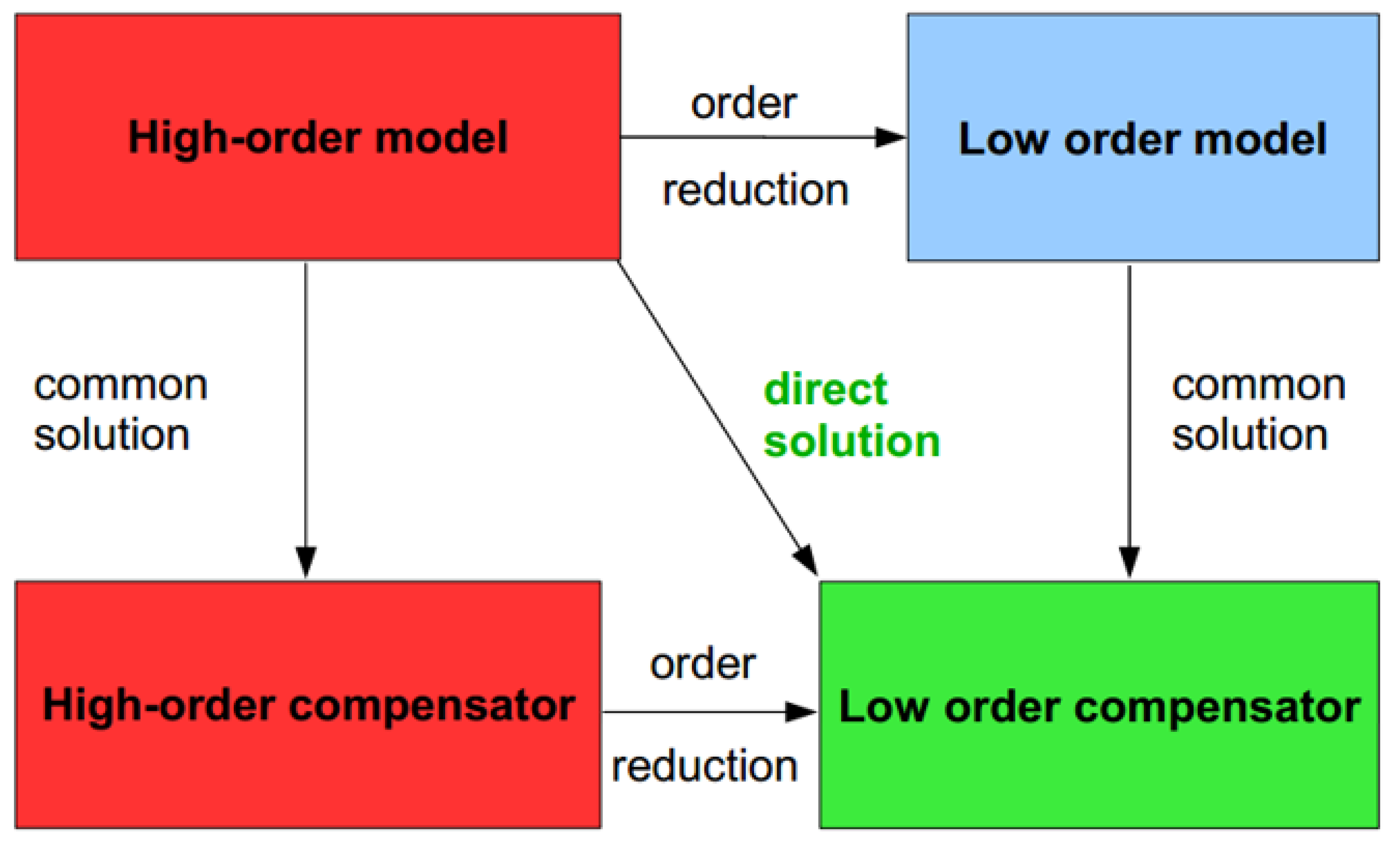
• Building, linearising and reducing a model of the system that has to be controlled. This can include a model of the uncertainty.
• Controller design with the reduced model.
• Simulation or co-simulation with the original non-linear model.

Each step may be executed by different engineers and may require different software tools. A disadvantage of many commercial software tools is that the reduced model obtained in Step 1 still needs a licence to run. Control engineers can then only use the reduced model if a costly licence is available. Models that can be used without a licence are clearly preferred.

The models need to be exchanged between the tools that are used in the different steps described above. The Functional Mock-up Interface (FMI) standard aims to be a standard for model exchange and co-simulation. Many tools support FMI import and/or export of models.

The central idea in step 1 is to make a model of a system with finite element software and find the best way to linearise, reduce and export this model to a FMI model. This workflow is schematically shown in Figure 4 along with the tools that were used: Abaqus, Python and OpenModelica. Of these tools, only Abaqus is a commercial software package. The reduced model is in standard state space form, so no Abaqus licences are required to run it.

The advantage of this approach is that the FEM model can be a very accurate description of the system, and it will be available for validation in Step 3 as well. The model reduction step will determine quite clearly which effects to include and which to exclude in the reduced model. Furthermore, if the system is built and measured, deviation between the model and system response can be attributed to parts of the system that were incorrectly produced (or incorrectly modelled).

This workflow is applied to the flexible arm benchmark in Section 3.2. The methods that were used (for step 1) are: finite element analysis, model order reduction, and FMU generation. These methods are discussed next.

2.3.1. Finite Element Analysis

A FEM model of the flexible arm mechanism is built with all structural details that are considered to be relevant. This includes the disk coupling between the motor and the shaft, for example. Once the model is made, it can be used in several analyses: transient (implicit or explicit), time-harmonic (called steady-state dynamics in Abaqus) or modal (calculation of eigenfrequencies and mode shapes).

The transient simulation may seem the most relevant for mechatronic design, but this analysis is computationally too expensive to be useful. It will only be used to validate the designed controller (in Step 3). The modal analysis is the most important one because it will yield the results that allow us to create a reduced order model.

2.3.2. Model Order Reduction

Several model order reduction (ROM) techniques are described in [27]. The Mode displacement technique is very commonly used for mechanical models and is implemented in most FEA sofware packages, including Abaqus. We want to take this a step further in two ways: automatic mode selection and model export (discussed in the next subsection).

The model is actually reduced twice: first by truncating all modes above a cutoff frequency, and next by using the Balaced truncation method; see also [27]. Balanced truncation is a ROM technique of its own, but in our two-step approach, it is reduced to a mode selection method. This method takes both input (actuator) and output (sensor) specification into account. For single-input singe output (SISO) systems, the mode selection can be done by looking at the mode shapes. However, for multiple-input–multiple-output (MIMO) systems, this becomes tedious and automatic mode selection is helpful.

2.3.3. FMU Model

As mentioned above, FEA software often includes some (ROM) methods. The problem with these methods is that running these ROMs requires a license of the FEA software. This is inconvenient and unreasonably costly (financially). Fortunately, as long as the ROM is linear, it is relatively straightforward to assemble the ROM outside the FEA software. Only the eigenfrequencies and mode shapes are needed and output of these is supported by all FEA software packages.

Assembling the ROM using the eigenfrequencies and mode shapes can be done in any software. We used Python, but Matlab may be the software of choice for a control engineer. Since the ROM is a linear model, it can be formulated in the standard state space form and can be exported as such. Therefore, FMU export is not really needed. Nevertheless, it can still be convenient to have a single FMU ROM that is used in all software environments (that support FMU). The FMU of a state space system can be conveniently created in Open Modelica using a predefined state space block.

2.3.4. Extension to Non-Linear ROMs

The described workflow from FE model to FMU works well for linear models. It can be extended to non-linear models only with much more difficulty (and further investigation).

A useful ROM technique for structural dynamics is substructuring. This is applicable if deformations remain small. Geometric non-linearity due to finite rotation is (mostly) accounted for. This technique is available in Abaqus and many other FEA programs. This leaves the problem that running the ROM needs a software license. Unlike in the linear case, the structure of this non-linear ROM resembles multibody equations that are nowhere near as simple as the linear ROM equations. Furthermore, extracting all the necessary data from the FE model is more difficult.

Non-linear ROMs with a simpler structure can also be used. For example, the model could be linearized around a nominal path. This linearization can be done either in time, resulting in a linear time-varying (LTV) system [28], or in parameter space, resulting in a linear parameter-varying (LPV) system [29]. In either case, extracting the required data from the FE model is not trivial. Furthermore, the ROM may need to be reassembled each time the nominal path is changed, which further complicates the workflow.

2.4. Data-Driven System Identification

Data-driven system identification is another widely used modelling approach. The model is constructed based on the information extracted from the experimental data. This allows high-fidelity models to be delivered from observations without relying on a detailed prior knowledge of geometry and physics involved in the dynamics of the controlled plant. The derived models are often directly applicable for the subsequent step of model-based control design. On the other hand, they often offer a limited insight into physical properties of the system under study. This may be necessary for qualified predictions regarding machine design changes made in the early phases of the development cycle. Moreover, a prototype has to be built physically to allow execution of experiments for data acquisition.

In our approach, we consider two different scenarios in which the data-driven identification may be used as a complement to the physics-based modelling:

• Experimental identification for direct derivation of a control-relevant model
  The first scenario is relevant for the final phases of machine construction, assembly and control system commissioning. The data gathered from an experiment with the real plant may often offer more information than first-principle models. This is due to several factors usually not taken into consideration when developing the analytical and FEM models such as actuator/sensor dynamics and noise characteristics, unknown material properties or construction tolerances, and varying assembly conditions, e.g., clamping, tightening, and friction forces. The first-principle models may be used to derive a proper structure of the control-relevant model, e.g., by estimating a number of oscillatory modes in the target bandwidth range. The data-driven identification provides parameters for the assumed model structure. The result is used for the subsequent control algorithm design.
• Experimental identification as a means for improving quality of the physics-based models
  This scenario involves early stages of development that often use various testbeds and prototype designs for the validation of predictions made by physics-based models. Employment of the experiments allows the geometrical or analytical models to be further refined. The location and damping of the eigenmodes acquired from the experiments may be used to tune material and geometrical properties in the first-principle models, extending their predictive and extrapolation capabilities. In this way, the amount of model uncertainty can be vastly reduced.

We focused mainly on the second scenario, which combines physics- and data-driven modelling approaches together. Our goal was to compare the results obtained from the analytical, FEM, and experimental models and provide some guidelines to the ways of incorporating the experimental results in the modelling process. Section 3 summarises our findings and recommendations in this context.

As for the data-driven identification, there is a wide variety of well-developed, tried and tested methods and algorithms available in the linear systems theory [1,2,3] that can be applied for this purpose. We opted for the frequency-domain modelling and identification framework outlined in [2], which provides some inherent advantages when used for flexible motion systems:

• Utilisation of deterministic periodic excitation signals for the experiments allowing to employ powerful averaging techniques to mitigate measurement noise and transient dynamics effects;
• Derivation of non-parametric frequency response function (FRF) as an intermediate step that may serve for model validation, providing a description of the oscillatory dynamics in a more natural way than time-domain models;
• Possibility of derivation of non-parametric noise models allowing model uncertainty to be evaluated;
• Numerically robust algorithms available for synthesis of the parametric transfer function models.

The workflow used in the identification experiment is illustrated in Figure 5 with the individual steps explained in the following sections.

2.4.1. Optimal Excitation Signal Generation

Utilisation of wide-band, deterministic, and periodic excitation signals is assumed for the identification experiments due to several advantages they inherently bring in the process of plant model derivation:

• Simultaneous excitation over the frequency band of interest resulting in shorter experiment duration;
• Improved signal-to-noise ratios compared to stochastic random noise excitations;
• Periodic nature allowing to measure multiple realisations of the executed motion trajectory to mitigate noise and transient leakage effects
• Possibility of optimisation of testing signal power spectrum, e.g., to minimise the resulting crest factor, shaping the energy fed to the feedback loop under closed-loop experimental conditions.

A multi-sine signal comprising the number of base harmonic functions with different frequency, amplitude, and phase delay is considered in the form of

$$r\left(t\right)=\sum _{k=1}^N{A}_{k}cos(2\pi k{f}_{0}t+{\phi }_k).$$

(20)

The amplitudes $A_k$ and spectrum $k{f}_0$ of the excitation trajectory can be optimised based on the requirements of the execution time of the experiment, required frequency resolution of the non-parametric model and assumed control bandwidth.

2.4.2. Non-Paramateric FRF Model Computation

The input and output data are measured and recorded over M multiple periods and broken into the corresponding set of sub-records. In case the measurement occurs under steady-state conditions, there will be no leakage due to the transients. The sample mean can be computed from the DFT spectra of the plant input and output signals

$$\overline{U}\left({\omega }_k\right)=\frac{1}{M}\sum _{l=1}^M{U}^{\left[l\right]}\left({\omega }_k\right),\overline{Y}\left({\omega }_k\right)=\frac{1}{M}\sum _{l=1}^M{Y}^{\left[l\right]}\left({\omega }_k\right),$$

(21)

with the corresponding (co)variances given as

$$\begin{array}{ccc}\hfill {\widehat{\sigma }}_U^2\left({\omega }_k\right)& =& \frac{1}{M-1}\sum _{l=1}^M{|U^{\left[l\right]}\left({\omega }_k\right)-\overline{U}\left({\omega }_k\right)|}^2,\hfill \end{array}$$

(22)

$$\begin{array}{ccc}\hfill {\widehat{\sigma }}_Y^2\left({\omega }_k\right)& =& \frac{1}{M-1}\sum _{l=1}^M{|Y^{\left[l\right]}\left({\omega }_k\right)-\overline{Y}\left({\omega }_k\right)|}^2,\hfill \end{array}$$

(23)

$$\begin{array}{ccc}\hfill {\widehat{\sigma }}_{YU}^2\left({\omega }_k\right)& =& \frac{1}{M-1}\sum _{l=1}^M(Y^{\left[l\right]}\left({\omega }_k\right)-\overline{Y}\left({\omega }_k\right)){(}{U}^{\left[l\right]}\left({\omega }_k\right)-\overline{U}\left({\omega }_k\right){)}.\hfill \end{array}$$

(24)

The FRF estimate is acquired from the division of the averaged output and input spectra

$$\widehat{P}=\frac{\overline{Y}}{\overline{U}}=\frac{Y_0+N_Y}{U_0+N_U},$$

(25)

where $Y_0,U_0$ denote the true spectra and the corresponding disturbance $N_Y,N_U$ introduced by the measurement errors. Bias and variance values of the resulting model can be obtained from the Taylor expansion of the previous equation under some assumptions about the input and output noise signals [2]

$$b=E\left\{\widehat{P}\right\}-P_0=-P_{0}exp(-M\frac{|U_0{|}^2}{{\sigma }_U^2})(1-\rho \frac{U_0/{\sigma }_U}{Y_0/{\sigma }_Y}),$$

(26)

where $\rho$ is the correlation between the input and output noises

$$\rho =\frac{{\sigma }_{YU}^2}{{\sigma }_Y{\sigma }_U},$$

(27)

and the variance estimate is obtained as

$${\sigma }_{\widehat{P}}^2=\frac{1}{M}{\left|P_0\right|}^2\left(\frac{{\sigma }_Y^2}{|Y_0{|}^2}+\frac{{\sigma }_U^2}{|U_0{|}^2}-2Re\left(\frac{{\sigma }_{YU}^2}{Y_0{U}_0}\right)\right).$$

(28)

It can be deduced that the relative bias gets reduced exponentially with the number of averaged periods and increasing SNR of the plant input. Careful preparation of the identification experiment by designing optimized wide-band signals and repeating a sufficient number of periods can be used to mitigate the bias effect. The same holds for the variance of the resulting FRF estimates. The variance expression can be used for the construction of the confidence intervals, which may serve in the subsequent phase of parametric modelling for the derivation of the model uncertainty. This information can be used for the robust controller design.

2.4.3. Complex Curve Fitting by Nonlinear Least Squares Optimisation

A second step of the identification follows once the FRF data have been obtained from the previous step. The problem of approximation of the complex data by a rational continuous- or discrete-time transfer function model

$$P(s,\theta )=\frac{b\left(s\right)}{a\left(s\right)}=\frac{{\sum }_{i=0}^{n_b}{b}_i{s}^i\left(s\right)}{s^{n_a}+{\sum }_{i=0}^{n_a-1}{a}_i{s}^i},P(z,\theta )=\frac{b\left(z\right)}{a\left(z\right)}=\frac{{\sum }_{i=0}^{n_b}{b}_i{z}^i\left(s\right)}{z^{n_a}+{\sum }_{i=0}^{n_a-1}{a}_i{z}^i},$$

(29)

with a vector of unknown coefficients

$$\theta =\{a_i;i=0,..,n_a-1,b_i;i=0,..,n_b\}.$$

(30)

can be formulated as an optimisation in the least-squares sense. The goal is to minimise the cost function

$$\begin{array}{ccc}& {\chi }^2\left(\theta \right)=\frac{1}{2}\sum _{i=1}^m{\left[\frac{r_i\left(\theta \right)}{w_i}\right]}^2=\frac{1}{2}r{\left(\theta \right)}^{T}Wr\left(\theta \right),{\theta }^{\ast }=\underset{\forall \theta }{argmin}\left\{{\chi }^2\left(\theta \right)\right\},& \hfill \\ & r\left(\theta \right)={\left[\begin{array}{cccc}{r}_1\left(\theta \right)& r_2\left(\theta \right)& \dots & r_m\left(\theta \right)\end{array}\right]}^T;r_l\left(\theta \right)=|P\left(i{\omega }_l\right)-\widehat{P}(i{\omega }_l,\theta )|,l=1..m\end{array}$$

(31)

The nonlinear least squares problem can be approximated by a series of simple linear subproblems

$$\begin{array}{cc}& {\chi }_{LLS}^2\left(\theta \right)=\frac{1}{2}{r}_{LLS}{\left(\theta \right)}^T{W}_L{r}_{LLS}\left(\theta \right),\\ & r_{LLSl}\left(\theta \right)=|P\left(i{\omega }_l\right)\widehat{A}\left(i{\omega }_l\right)-\widehat{B}(i{\omega }_l,\theta )|,l=1..n_f,\widehat{P}\left(i\omega \right)=\frac{\widehat{B}\left(i\omega \right)}{\widehat{A}\left(i\omega \right)}.\end{array}$$

An iterative procedure is formed by finding a linear least-squares estimate in each step as

$$\begin{array}{c}\hfill {\theta }_{k+1}^{\ast }=\underset{\forall \theta }{argmin}\left\{\frac{1}{2}{r}_{LLS}^T\left(\theta \right)W_k{r}_{LLS}\left(\theta \right)\right\},\end{array}$$

(32)

with the weights $W_k$ adjusted to the uncertainty of the individual samples of the non-parametric model to form a maximum-likelihood estimate.

The result of this step is used as an initial guess for the subsequent nonlinear optimisation. In our application, the Levenberg–Marquardt method [30] is employed to solve the nonlinear least squares problem. Orthogonal parameterisation of the transfer function polynomials is used to improve numerical conditioning of the problem. The reader is referred to publication [2] for a detailed treatment of the identification topic.

2.5. Robust Control Design

There is a lack of generic theoretical methods supporting simple design of low-order fixed-structure controllers, which are dominantly used in industrial motion control systems. Generally accepted methods of modern control theory usually lead to high-order controllers (the controller order is typically higher or equal to the order of the controlled plant), which are inherently difficult to tune and implement in practice. The usual approach to the fixed-structure controller design is to perform an order reduction either for the plant model or for the derived high-order controller (Figure 6).

This inevitably leads to some performance loss resulting from the performed approximation. Direct methods usually rely on numerical non-convex optimisation resulting in no guarantee of convergence and global optimality of the derived results [31]. A generic approach to design of PID controllers, that are prevalent in industrial motion control hardware, is still missing. A new design method specifically tailored to PID controllers was developed at our workplace recently in an attempt to fill this gap between the academic research and practice [32]. It is primarily intended for PI(D) controllers and simple fixed-structure feedback control algorithms with two or three parameters (lead-lag compensators, low-order static feedback etc.).

The basic features of this approach are summarised as follows:

• Formulation of the design specifications in the frequency domain by imposing arbitrary closed-loop weighted sensitivity inequalities;
• Possibility of automatic calculations for the auto-tuning purposes;
• Generic method for an arbitrary LTI system described by a rational transfer function + time delay;
• Suitable for robust controller design using structured or unstructured uncertainty models;
• Analytical method for the computation of the admissible set of controllers, no performance losses due to approximations, model reduction or non-convex numerical optimisation.

A brief review of the main results is added in the following section for the sake of compactness. Examples of employment of this approach in motion control system design problems are given in references [13,33].

H-Infinity Loop-Shaping Design of a Fixed-Structure Controller

The starting point is a model of a generic controlled process $P\left(s\right)$ without the poles on the imaginary axis (can be relaxed by adjusting the controller derivation procedure). The feedback compensator $C\left(s\right)$ is considered in the standard PI controller form

$$C(s,k)=k_p+\frac{k_i}{s},$$

(33)

where k denotes the parameters vector $[k_p,k_i]$.

An arbitrary number of design constraints can be formulated in the frequency domain as loop-shaping inequalities in the form of

$${\left|\right|H(s,k)\left|\right|}_{\infty }<\gamma ;H(s,k)\stackrel{\Delta }{=}W\left(s\right)S_{\ast }\left(s\right),$$

(34)

where $S_{\ast }\left(s\right)$ denotes one of the closed-loop sensitivity functions (sensitivity, complementary-, input-, and controller-sensitivity, respectively—see Figure 7 for the physical meaning in terms of the loop input and output signals), $W\left(s\right)$ introduces an arbitrary user-defined frequency-dependent scaling, and $\gamma$ is a scalar design parameter.

The goal is to find a controller $C(s,k)$, which, together with the given $H\left(s\right)$, fulfils the following three conditions

• $C(s,k)$ internally stabilises the closed-loop;
• $H(s,k)$ used in the design criterion is stable;
• The H-infinity condition ${\left|\right|H(s,k)\left|\right|}_{\infty }<\gamma$ holds.

This controller is called the $H_{\infty }$controller. Typically, there is a whole set of the admissible controllers fulfilling the above-mentioned conditions, which can be represented directly in the parametric plane $[k_i,k_p]$ (Figure 8).

This boundary defines a set of admissible controllers. In case the set is nonempty, which means that there exists at least one controller of the given structure for the defined design constraint, one particular parameter combination has to be chosen. One of the possible choices is to select the controller with the highest integral gain, which is known to minimise the Integral error criterion

$$IE={\int }_0^{+\infty }e\left(t\right)\mathrm{d}t=\frac{1}{k_i}.$$

(35)

The computation of the $H_{\infty }$ region and its corresponding set of admissible controllers is a nontrivial task. However, as shown in [32], an explicit solution can be derived in the form of

$$\begin{array}{cc}\hfill k_i\left(\omega \right)& =F_i(\omega ,x_l,\gamma ),\hfill \\ \hfill k_p\left(\omega \right)& =F_p(\omega ,x_l,\gamma ,A,B,A_1,B_1,w,w_1),\hfill \\ \hfill \omega & \in [0,\infty ),\hfill \end{array}$$

(36)

with the arguments of parametric curves $F_i,F_p$ defined as

$$\begin{array}{cc}\hfill A& \stackrel{\Delta }{=}Re\left(P\left(j\omega \right)\right),A_1\stackrel{\Delta }{=}\frac{\mathrm{d}A}{\mathrm{d}\omega },\hfill \\ \hfill B& \stackrel{\Delta }{=}Im\left(P\left(j\omega \right)\right),B_1\stackrel{\Delta }{=}\frac{\mathrm{d}B}{\mathrm{d}\omega },\hfill \\ \hfill w& \stackrel{\Delta }{=}{\left|W\left(j\omega \right)\right|}^2,w_1\stackrel{\Delta }{=}\frac{\mathrm{d}w}{\mathrm{d}\omega },\hfill \end{array}$$

(37)

and $x_l;l=\{1,2,3,4\}$ are the real roots of the “companion” polynomial

$$a{x}^4+b{x}^3+c{x}^2+dx+e=0,$$

(38)

with the real coefficients $a,b,c,d,e$ depending explicitly on $\{\omega ,x_l,\gamma ,A,B,A_1,B_1,w,w_1\}$ (see the reference [32] for the full derivation). The important result is that the computation of the $H_{\infty }$ region always leads to a 4th-order polynomial regardless of the order of the plant or the user-defined weighting functions. Therefore, analytic expression for its roots is available from the Ferrari’s method and Cardano formulas. Their careful examination allows a separation of the real roots which lead to the solution of the $H_{\infty }$ region boundary.

Multiple design constraints may be formulated in the frequency domain for several weighted $H_{\infty }$ norm of various closed-loop sensitivity functions. The resulting admissible region is then computed from the intersection of the individual regions corresponding to each design constraint. Computer software automating the derivation of the parametric regions has been recently developed; see [34]. A publicly available version will be released soon.

3. Results

This section presents the results of application of the previously described methods on the formulated benchmark problem of flexible manipulator modelling and control. The first part deals with the development of physics-based models using analytical and FEM approaches. These first-principle models are then validated using the experimentally measured data. A loop is formed in the modelling cycle, allowing the adjustment of geometrical and mechanical properties of the FEM model based on the experimental observations. Control-relevant parametric model is subsequently derived using the proposed techniques of order reduction and linearisation. The mentioned control design method is used to synthesise a robust controller that is to be used for a whole set of manipulator configurations with variable load mass geometry. Experimental results show effectiveness of the closed-loop control and also provide means for comparison of reduced linear and full-scale 3D nonlinear numerical simulations.

3.1. Analytical Model Development Using Euler–Bernoulli Beam Theory

As we outlined in the previous sections, a simple mathematical model may give some primary useful insight into the dominant system eigenmodes. The computed dynamical behaviour can be used in simulation prior to assembling the physical setup and can therefore help to redesign it. Let us suppose that we have just some principal idea about the machine construction, material, and purpose of application, and we would like to get some initial insight into its dynamical behaviour. Considering this, we include just the fundamental parts of the complex construction to the dynamical model descriptio. In addition, in the mathematical model. the arm length, the payload position, or the mass can be easily modified to visualise the impact on the dynamical behaviour of such possible changes. The whole set of models can thus be validated and investigated thoroughly.

The Lagrange–Euler method [20] with the Euler–Bernoulli theory [21,26] can be now employed. We shall start with the following formula

$$\frac{d}{dt}\frac{\partial L}{\partial \dot{q}}-\frac{\partial L}{\partial q}={\mathcal{T}}_m,$$

(39)

where in the Lagrangian $L=T-V$, the kinetic energy T and potential energy V are subtracted. ${\mathcal{T}}_m$ denotes the torque vector, and q is the state co-ordinates vector. In this modelling case study, the energies of the hub and payload are taken into account as well as the energy of the arm that is divided into four elements. Therefore, the state co-ordinates vector can be established as $q={\left[\begin{array}{cccc}\theta & q_1& \dots & q_{10}\end{array}\right]}^T$, where $\theta$ is the hub angle and $q_i$ denotes for the ith element the displacement (if i is odd) and the angle (if i is even).

Specifically, the kinetic energy of the hub is considered simply as $T_h=\frac{1}{2}{J}_h{\dot{\theta }}^2,$ where $J_h$ is the hub inertia moment. The energy of the payload ($T_p$) and the energies of the arm elements ($T_i$, $V_i$) depend on the deflection function $u(x,t)$ outlined in (2). The payload is considered as a concentrated mass located on the last element, i.e., $s=l$. This leads to

$$T_p=\frac{1}{2}{m}_z{\dot{u}}^2{(l,t)|}_{j=n+1},$$

(40)

where $m_z$ is the mass of the payload, ${\left.\dot{u}(l,t)\right|}_{j=n+1}=\overline{N}(l,t)\dot{\overline{Q}}\left(t\right)=nl\dot{\theta }\left(t\right)+{\dot{q}}_{2n+1}\left(t\right)$. Specifically, the payload mass is located at the last element, i.e., $n=4$, and is related to the variable $q_9$. The energies of the arm are considered as (12) for $n=4$. By summing energies of all considered components, we obtain

$$T=\sum _{i=1}^4{T}_i+T_h+T_p,V=\sum _{i=1}^4{V}_i.$$

(41)

Thus, we can complete the Lagrange–Euler method and derive the system of the second ordinary differential equations for the Lagrangian $L=T-V$, where T and V are given as (41). This system can also be expressed as the mechanical equation

$$M\left(q\right)\ddot{q}+Kq=b\tau ,$$

(42)

where $M\left(q\right)$ is the mass matrix, K is the stiffness matrix, and $\tau \in R$ is the input torque, $b={\left[\begin{array}{cccc}1& 0& \dots & 0\end{array}\right]}^T$.

These formulas are moreover restricted by the condition on the arm attachment. When the arm is modelled with one fixed end and one free end, the variables $q_1,q_2,{\dot{q}}_1,{\dot{q}}_2$ vanish. Hence, the adjusted state co-ordinates vector becomes

$$q={\left[\begin{array}{cccc}\theta & q_3& \dots & q_{10}\end{array}\right]}^T.$$

(43)

We obtain nonlinear differential equations and linearise them in the equilibrium point ${\left[\begin{array}{cccc}0& 0& \dots & 0\end{array}\right]}^T$. We derive the state-space model for the state vector $z={\left[\begin{array}{cccccccc}\theta & q_3& \dots & q_{10}& \dot{\theta }& {\dot{q}}_3& \dots & {\dot{q}}_{10}\end{array}\right]}^T\in R^{18}$ as

$$\dot{z}=\left[\begin{array}{cc}0& I\\ -M^{-1}K& 0\end{array}\right]z+\left[\begin{array}{c}0\\ M^{-1}b\end{array}\right]\tau .$$

(44)

The displacement of the payload can be expressed as

$$y=L{z}_1+z_8.$$

(45)

This elementary stage of the modelling can be useful to obtain some basic knowledge about the eigenmodes. From the linearised model, by substituting the parameters according to Table 2, the plant model poles can be calculated as follows:

$$\left\{0,0,\pm 339.07\mathrm{j},\pm 1281.10\mathrm{j},\pm 4174.98\mathrm{j},\pm 8709.23\mathrm{j},\pm 16372.05\mathrm{j},\pm 26653.93\mathrm{j},\pm 42495.65\mathrm{j},\pm 63216.13\mathrm{j}\right\}.$$

As shown in the comparison in the following sections, the first two eigenmodes are sufficiently comparable with the more precise models developed using FEA software.

3.2. Workflow Using Commercial FEA Software

There are many FEM software packages, including free and open source ones. Commercial FEA software (OOFELIE or Abaqus, for example) typically has benefits such as support, backwards compatibility, user-friendliness, and well-developed pre- and post-processing interfaces. Possible drawbacks of commercial software, beside costs, are limited output/export possibilities. Nevertheless, standard output already gives many possibilities for use in a mechatronic design workflow. An example is given in this subsection.

3.2.1. FEM Model and Linearization

A FEM model of the mechanism shown in Figure 1 is made in Abaqus. Figure 9 shows the model with all part names.

The input of this model is the motor torque and the outputs are the y-displacement at the tip of the arm and the angle and angular velocity of the motor.

The arm, base plate, spacer, and the two disk-coupling plates are modelled as flexible components using shell elements. The shaft and hub are also flexible, but modelled using beam and continuum elements, respectively. All flexible parts are made of steel. A linear elastic material model is used; initially without damping.

The mass, flywheel, and clamp are rigid and modelled with discrete rigid elements. The rotor and stator of the motor are rigid too, but modelled with point inertias. A connector element between stator and rotor keeps these parts aligned, and allows one to specify the motor torque and conveniently extract relative rotation (or vice versa). The model is input torque which is directly proportional to motor current. Besides this gain, no further motor parameters are needed.

Bearings are also modelled using connectors. Torque is zero for these of course. The location of the bearings can be seen in the coupling plot, Figure 9 (right). The couplings are the red lines. From top to bottom: clamp to shaft and mass to arm; upper bearing to hub; lower bearing to hub; disc coupling plates to shaft, to each other, and to the rotor; and last, stator to cage. The model does not use contact interactions.

The model is clearly non-linear because of the large rotations that are possible. Linearization of the model is done in the position shown in Figure 9 (left). The velocity is zero for this model state. Therefore, the linearized model will be accurate for low rotational velocities only.

The fifty lowest eigenfrequencies and eigenmodes are calculated in Abaqus. The first eigenmode is the rotational rigid body mode. Mode 2 and 3 are shown in Figure 10.

If measuring the system is not possible, then damping can be added to the FEM model. However, modelling damping is not trivial; see for example [35]. Therefore, a practical shortcut is taken here. Damping was not included in the FEM model (before linearization and reduction). Instead, modal damping was added to the reduced model. Realistic damping values are identified later from experimental measurements acquired from the system.

3.2.2. Model Reduction

The fifty modes that were calculated are not all equally relevant for the input/output relations of the system. For example, mode 2 in Figure 10 is important, and mode 3 in the same figure is not. Mode shapes that are large at both the input(s) and the output(s) are relevant. Therefore, one way to proceed with the model reduction is to select the most important modes by just looking at the mode shapes. This works quite well in the SISO case, but becomes tedious if the system has multiple inputs and/or outputs.

Automation or at least guidance of the mode selection is possible by using balanced truncation. Balanced truncation is a model order reduction technique in itself, developed in the field of systems and control [27]. It specifically aims to reduce the model while keeping the accuracy of the input/output relations as high as possible. This contrasts with the mode displacement method that is not aware of inputs and outputs.

A limitation of balanced truncation is that it can only be applied to models up to 1000 degrees of freedom (DOFs); FEM models typically have many more. To overcome this limitation, the reduction strategy consists of two steps:

• Initial reduction using the mode displacement method and all modes up to some frequency that is considered to be high enough.
• Secondary reduction by balanced truncation. This turns balanced truncation into a mode selection method.

The balanced truncation method usually selects linear combinations of the degrees of freedom of the model that it is applied to. Figure 11 shows an example: 11 Balanced truncation DOFs are chosen (or actually 22 first order DOFs), resulting in 11 modes selected from the modal displacement model.

The resulting transfer functions of the reduced model are shown in Figure 12. The results are accurate up to 1 kHz. Peaks above 1 kHz are neglected in the reduced model, but this is acceptable.

Figure 13 compares the reduced order model, with added modal damping, to measurements. The amount of damping could be tuned further, but the current match is acceptable. Overall, the match is quite good, except for the peak near 150 Hz. The mode shape that corresponds to this peak suggests that shaft and/or disk coupling is too flexible in reality, or too stiff in the model. It can be seen that the resonances around 1 kHz frequency are not captured well by the model. Further investigation of this mismatch revealed that the real plant exhibits additional bending modes of the manipulator base frame that was not included in the geometry of the FEM model. However, this high-frequency dynamics lies far beyond achievable target bandwidth and thus was decided to be left unmodelled. The derived model achieves a very good match for frequencies up to 500 Hz, which is more than satisfactory for the purpose of control design in our case.

Figure 14 compares both derived 1st principle models with the experimental data. It can be seen that the analytical model based on the Euler–Bernoulli beam theory is able to capture first-smode dynamics very well. There is a mismatch of about $25\%$ in the location of the second resonance frequency. The higher bending modes are not modelled well for several reasons:

• Overly simplistic point two-mass model of the actuator and arm connection that is a source of the oscillatory dynamics around 500 Hz;
• Neglected machine frame dynamics (as in the case of the FEM model).

The achieved result shows typical weakness of the analytical modelling approach. Although it may work for simple mechanisms, its applicability seems limited for complex machine geometries. Therefore, we decided to use only the reduced order model acquired from the geometric FEM and proceeded with its validation in a closed-loop setting.

3.3. Combining First-Principle Models with Experimental Observations

The process of development of a mechatronic system usually consists of several subsequent phases. Preliminary analysis and machine design are usually followed by a detailed elaboration of mechanical construction, today with the aid of computer software. Control-related questions may arise in this phase by analysing basic dynamic properties using FEA methods. Adjustment of the design choices may be needed to deliver favourable dynamic properties to fulfil formulated control objectives. Assembly of a prototype is often necessary for validation of the machine design. Data acquired from experiments with a real machine may provide invaluable information relevant both for the purpose of control and for improvement of the fidelity of virtual models. The Digital Twin concept extends this approach by proposing to instance the virtual model according to specific machine samples which may differ considerably due to construction tolerances, assembly, differences in installation site, mechanical wear, and ageing of individual components. The virtual models can live parallel lives with their physical counterparts, being continuously updated with available observation data and providing improved predictions of machine performance and remaining lifetime. A fundamental question is which data may be used for improving the fidelity of physics-based models from the perspective of control-relevant predictions. This section provides some insights regarding this topic.

Figure 15 shows the model–measurement loop. Deviations between modelled and measured responses could indicate that either the real system does not function as designed or the model is not accurate enough. The first scenario may be relevant for the case of long-term operation of a machine that starts showing signs of wear or malfunction. However, we are now interested more in the early phases of the design cycle, which deals with validation of geometric models using data acquired from first experiments with assembled prototypes. Both the model and the actual system can be improved by completing this loop a few times. How we used this loop for stiffness, damping, and machine geometry in our flexible manipulator benchmark problem is discussed below.

3.4. Geometry and Stiffness

In one of the first comparisons of the FEM model with experimental data, we detected a resonance frequency mismatch. Several peaks in the response were shifted. The responsible mode shapes can be looked up in the modal FEA results. Next, a hypothesis can be formulated for the cause of the deviation and this cause can be tested using the FE model.

In our case, we suspected the clamping of the mass to the arm of the mechanism. The contact area that could be in contact was large and therefore not well defined. Reduction of the contact area in the model could cause a similar shift of the eigenfrequency as observed in the measurements. The mass of the mechanism was modified to reduce the potential variability of the contact surface. Figure 16 shows the modification. The modification has improved the match between model and measurements.

Still, there was some mismatch between the modelled and measured response. This could have been caused either by the disk coupling between the motor and the shaft or by the way we attached bearings and flywheel to the shaft. In either case, the model was too stiff. We have reduced the mismatch by lowering the stiffness of the disk coupling, because this was easy to do. This issue could have been investigated more accurately. However, it turned out to be a minor issue from the control performance perspective. Analysis of achievable closed-loop properties has shown that the first mode is a dominant precursor of the achievable bandwidth, and careful design of robust controller may mitigate high-frequency modelling errors far beyond the target closed-loop bandwidth.

3.5. Damping

We chose to tune damping in the model based on the measured response. While FEA allows different ways to specify damping, localised or material, it is difficult to specify it accurately; see for example [35]. Damping is expected to be low, so using no damping only results in small errors. These are important nevertheless, as we will see when the controller is validated.

Setting the damping in the reduced order model (ROM) is very simple. Since the ROM is based on the eigenmodes, modal damping can be set with single parameter for all eigenmodes or, if needed, with a parameter for each mode independently.

Modal damping is similar to viscous damping, but applied to a single mode. There is no equivalent type of damping available for transient simulation with the FE model. Rayleigh damping is the only available kind of global damping for transient simulations in Abaqus. This means that the damping is derived from the mass matrix (alpha damping), the stiffness matrix (beta damping), or a combination. This kind of damping is frequency-dependent, while viscous damping causes a constant damping ratio over the entire frequency range. Consequently, we need to be careful with damping when the controller is applied to the full model for validation. Adjustment of the damping based on the experimental data allowed us to achieve the model responses previously shown in Figure 13, further improving the intermediate results achieved by stiffness and geometry corrections demonstrated in Figure 17. The resulting model was used in the subsequent step of controller synthesis.

3.6. Load-Mass Parametric Uncertainty Modelling

Many mechatronic systems are employed in uncertain operating conditions affecting their overall dynamic response. A typical example is variable machine geometry within admissible work space or changes in the mass, inertia or position of the attached load. A fundamental issue from the control perspective is then the proper development of robust feedback loops capable of preserving certain closed-loop performance under all assumed plant variations.

A parameter variation scenario was formulated in order to evaluate the extrapolation capability of the developed full-scale geometric FEM model and test the proposed robust control method. The position of the attached mass was chosen as a variable parameter, which can reach any value in the interval between 180 mm and 200 mm, simulating either a change in the attached load, multiple existing variants derived from one machine design, or a second degree of freedom of the flexible arm manipulator; see Figure 18. This uncertainty affects the location of the oscillatory modes, mainly in the low-frequency range corresponding to arm bending modes, as shown in Figure 19. It is worth mentioning that an accurate physics-based model is needed for delivering this kind of extrapolation due to parameter variations. To acquire the same result from the experiments with a real plant, a wholse set of prototypes or lengthy experiments with variable machine configuration would be required. This may be relatively simple for our model benchmark scenario but may turn out to be infeasible in other practical applications. The role of high-fidelity full-scale nonlinear model is crucial in this case.

3.7. Model-Based Robust Feedback Control Design

A robust controller needs to be derived for the whole set of admissible plant models formed in the variable mass position scenario. For this sake, the $H_{\infty }$ method outlined in the previous sections was used. A method of gridding was applied to compute five representative linearised and reduced-order control-relevant models, with the load-mass position being sampled at points

$$l=\{180,185,190,195,200\}mm,P_k\left(s\right)=\frac{{\omega }_m\left(s\right)}{T_m\left(s\right)}{=P\left(s\right)|}_{l=l_k};k=1..5,$$

(46)

with the five transfer functions describing the dynamics between the torque applied by the actuator $T_m$ and angular velocity observed at the actuator side ${\omega }_m$. Linear models of order 25 were obtained containing 11 dominant flexible modes, one rigid mode of the system, and second-order actuator dynamics appended at the plant input due to the internal current control loop.

A standard fixed-structure PI controller (33), which is implemented in most of industrial servo-amplifiers, was assumed to close the velocity control loop. Only the first flexible mode of the system can be stabilised actively due to the low order of the compensator. The reader is referred to our previous work with a more thorough discussion of achievable performance in flexible motion systems equipped with PID controllers [14,36]. Therefore, the controller is complemented by a notch-filter and low-pass filter to improve its high-frequency roll-off to improve achievable closed-loop bandwidth and avoid unwanted destabilisation due to higher bending modes, resulting in controller transfer function in the form of

$$C\left(s\right)=\frac{T_m\left(s\right)}{e_{\omega }\left(s\right)}=\left(k_p+\frac{k_i}{s}\right)\left(\frac{s^2+2\xi {\omega }_n+{\omega }_n^2}{s^2+2{\omega }_n+{\omega }_n^2}\right)\left(\frac{{\omega }_f^2}{s^2+\sqrt{2}{\omega }_{f}s+{\omega }_f^2}\right),$$

(47)

where $T_m$ denotes the torque demand and $e_{\omega }$ is the velocity tracking error. The notch filter was tuned for the resonance frequency of $w_n$ = 2640 rad/s corresponding to actuator-arm bending mode to avoid its excitation. The bandwidth of the 2nd order Butterworth low-pass filter was set to $w_f$ = 4750 rad/s to cover the rest of the high-frequency flexible dynamics.

The design problem for the derivation of the PI gains in the controller (47) is formulated as a loop-shaping inequality

$$M_S=\left|\right|S_k{\left|\right|}_{\infty }=\underset{\forall \omega }{sup}\left|S_k\left(j\omega \right)\right|<1.4\forall k=1..5;S_k\left(s\right)=\frac{1}{1+C\left(s\right)P_k\left(s\right)},$$

(48)

with $S_k$ denoting the closed-loop sensitivity function obtained from the fixed-structure controller (47) and all the plant models in (46).

The design requirement (48) enforces a specified closed-loop stability margin $s_m$, because the $M_S$ value is indirectly proportional to a closest distance at which the open-loop Nyquist plot approaches the critical point $[-1,j0]$ in the complex plane

$$\frac{1}{M_S}=s_m=\underset{\forall \omega }{inf}|1-L\left(j\omega \right)|,L\left(j\omega \right)=C\left(j\omega \right)P\left(j\omega \right),$$

(49)

thus directly affecting the amount of uncertainty the loop can handle before getting unstable in the closed-loop setting. This is a special case of the generic requirement (34) that can be handled with the aforementioned $H_{\infty }$ regions method. The set of admissible controllers is computed and visualised in the parametric $k_p-k_i$ plane in Figure 20 using the software tool from [34].

Different regions are computed for each member of the plant models set defined by (46). The intersection of all the regions defines the admissible set of controllers fulfilling the design requirement (48) for all the plant models simultaneously. An infinite number of controllers exist, and one particular combination of parameters has to be chosen for practical implementation. One possible choice is the point with the highest achievable integral gain (the red point designated in Figure 20), which is known to minimise the integral error criterion evaluating the evolution of tracking error under step input disturbance excitation; see Equation (35). This leads to the PI gain values of $k_p=74.9,k_i=188.2$. Alternatively, any other suitable criterion could be chosen, leading to possible other points in the admissible set.

The fulfilment of the design objectives (48) can easily be checked by evaluating the closed-loop sensitivity function $\left|S\right(j\omega \left)\right|$ for the model set in (46). As shown in Figure 21, the maximum sensitivity requirement is fulfilled, delivering a robust controller for the assumed parametric variations. The second peak around 3000 rad/s signals potential closed-loop issues with high-frequency dynamics coming from the actuator and base support bending modes limiting the achievable bandwidth. It should be noted at this point that optimisation and fine-tuning of closed-loop performance for our particular benchmark system was not our primary goal. Our intention was merely to demonstrate the overall workflow and use the resulting controller for the evaluation of closed-loop performance predictions acquired from the derived models.

Analysis of the results showing the open-loop plant responses in Figure 19, parametric regions in Figure 20, and achieved closed-loop sensitivities from Figure 21 reveals that the highest load-mass distance of l = 200 mm is the most detrimental case for the range of applicable controller gains and at the same time achievable closed-loop performance. This is due to the fact that longer mass radius shifts the first resonance modes towards lower frequencies, which comes with more significant phase-delay introduced in the open-loop dynamics. It turns out for our particular parametric variation scenario that the optimal controller valid for the highest mass distance automatically fulfils the design requirements for the shorter strokes. This demonstrates that the derivation of the $H_{\infty }$ sets of admissible controllers can provide very useful insight into closed-loop behaviour and achievable performance. Figure 22 evaluates achieved closed-loop performance in terms of reference-following and disturbance-rejection experiment. It can be seen that the derived robust controller is able to achieve consistent performance under assumed parametric variations. Flexible modes of the arm are well-damped in both experiments. The input disturbance test reveals initial oscillations that are due to the flexible motor-arm coupling. This mode cannot be attenuated actively by the feedback compensator because of the notch-filter tuned for the respective resonance frequency. However, this is not a major limitation since load side disturbances are usually expected in practical motion systems. The reason for using input disturbance test was due to simple injection of additive torque by the actuator leading to repeatable experiments. Another motivation was the possibility of excitation of high-frequency dynamics, which is beneficial for evaluation of derived models’ fidelity. This topic is studied in the next section.

3.8. Experimental Closed-Loop Validation

The last step of the control design process was the validation of the derived compensator. The linear closed-loop simulation using linearised ROM was compared with the result of full-scale nonlinear FEM simulation and experiment with the physical setup.

As introduced in Section 2.3, one of the benefits of having an accurate FEM model is that it can be used to check the controller (step 3). The controller was designed on a simplified model in which several phenomena were neglected—centrifugal force, for example.

The designed controller can be included in the FEM software to check if it still functions as intended. In Abaqus, this has been done by implementing the discrete time version of the controller in an Abaqus user subroutine (UAMP). The transient dynamic model is solved using fixed time stepping at the controller sampling rate. This will take a while for large models, but in this case it is manageable. For larger models, if necessary, the efficiency can be increased by using intermediate-fidelity models with substructures, for example.

The first test of the controller was unsuccessful. The controller became unstable. The reason is that a small amount of damping is needed for a stable closed loop system. The full model did not yet include any damping, and the numerical damping of the time integration was too small, with the small time steps that are used. Adding damping solved these issues. There is no direct equivalent in transient simulations of viscous model damping (which was used to make the reduced model match the measurements). A solution is to apply beta material damping (stiffness proportional) and match the damping ratio of the viscous modal damping at the unstable frequency observed in the simulation without damping (171 Hz). This solution is not ideal, because higher frequencies will be damped more and lower frequencies less. Nevertheless, the damping at the problematic frequency is accurate, and this matters most. This approach worked well for our purposes. As discussed in Section 2.3, more accurate modelling of damping is possible but not simple.

Figure 23 shows a comparison of linear and nonlinear numerical simulations with actual experiment with the real motion stage for a particular case of load mass position of l = 200 mm that was identified as a worst case for achievable performance in the controller design phase. There is a very good match between the actual and predicted closed-loop behaviour, both for the linear and nonlinear simulation. The detail of the initial part of the transient on the right plot reveals a better fidelity of the nonlinear model. The linear model response shows an initial peaking phenomenon during the first ten milliseconds which is actually not observed in real plant data. The corresponding frequency of approximately 155 Hz indicates its relevance with the second bending mode of the flexible arm. The discrepancy in the observed behaviour might be caused by nonlinear effects not captured in the linear model or slight mismatch in the damping of the eigenmode in the linear model. Furthermore, further evolution of the initial oscillations during the first seventy milliseconds are captured better by the nonlinear simulation. On the other hand, the computational complexity aspect for both models should also be considered. While the linear simulation takes few seconds to numerically integrate the associated ordinary differential equations, the nonlinear simulation requires several hours and specialised numerical solvers. The overall shape of the response shows that both reduced and full-scale nonlinear models provide very good predictions of closed-loop performance. Very similar results were obtained for other mass positions and for varying amplitude of the step reference change. They are not presented here for the sake of brevity.

Additionally, a disturbance rejection case was modelled using a similar simulation setup in Abaqus and compared with the linear simulation and experimental data. Step torque was injected using the actuator by adding it to the controller output to excite the system and evaluate its disturbance rejection capability. The results are shown in Figure 24. The overall shape of the response reveals well-behaved closed-loop performance. The feedback loop is capable of attenuating all the unwanted flexible arm vibrations and settle the whole system. There are some transient oscillations during the initial phase as shown in the right detailed plot of Figure 24. This part is mainly affected by the high-frequency bending modes of the motor-arm coupling and base plate dynamics. The comparison of linear and nonlinear simulation confirms the previous results obtained from the reference-following test. The nonlinear simulation captures the high-frequency dynamics more closely at the cost of much higher computational demands. From the control perspective, the reduced-order linearised model is still capable providing high-fidelity predictions of both open- and closed-loop plant responses.

Figure 25 shows a comparison of linear and nonlinear simulation in terms of prediction error between the modelled closed-loop response and experimental results. In both cases, the full-scale FEM transient modelling provided more accurate predictions.

Table 3. Comparison of average and worst-case prediction error of linear and nonlinear model in the closed-loop reference-following and disturbance rejection experiments

	Reference Following		Disturbance Rejection
	$e_{rms}$	$e_{pk-pk}$	$e_{rms}$	$e_{pk-pk}$
Linear ROM	0.0455	0.405	5.82	40
Full scale nonlinear FEM	0.0449	0.279	3.05	31.7

quantifies average and worst-case values of the prediction error in terms of the root-mean-square and peak-to-peak indices

$$e_{rms}=\sqrt{{\sum }_{k=1}^N{e}^2\left(k\right)/N},e_{pk-pk}=\underset{\forall k}{max\left(e\right(k\left)\right)}-\underset{\forall k}{min\left(e\right(k\left)\right)}.$$

(50)

The difference is more pronounced in the disturbance rejection test because of more significant excitation of high-frequency dynamics of the machine frame and actuator-arm coupling. We conclude that from the control-relevance perspective, the reduced-order linear model also proved to be very capable for both numerical simulations and robust controller design. The nonlinear dynamic effects would be pronounced more for higher rotational velocities and driving torque amplitudes. Nevertheless, the difference is minor for the assumed operational regimes of the physical plant due to practical actuator and construction constraints.

In order to obtain the results for Figure 24 and Figure 25, we needed to redistribute the stiffness between the disk coupling and the shaft. Otherwise, the disk coupling would buckle. The linear model in these figures has not been updated, but a linearised version of the updated full model would be very similar. The buckling problem was not present at the excitation levels for Figure 23. If the full model should be able to predict a loss of linearity, then the disk-coupling part of the model needs further validation. However, this was not necessary for our purposes of control-relevant modelling. These issues show that the full model does not need to be perfect in order to be valuable. Incremental model updates can be made when the situation demands them.

3.9. Additional Validation: Extended Range of Solicitations for Disturbance Rejection Test

Further experiments with numerical simulations were made to reveal potential limits of validity of the linear reduced order model. In parallel to the full NL 3D model that was performed in Abaqus, some full NL 3D mechatronic simulations were also performed using OOFELIE::Multiphysics. The model was slightly simplified to reduce computational complexity, but the model stays close to the one that was prepared in Abaqus. For example, the model in OOFELIE::Multiphysics introduces the following simplifications:

• The spacer and the base plate were considered as clamped.
• The Cardan joint was simplified. Each of the two Cardan discs was replaced by a hinge with an internal rotation spring. The stiffness of this spring was updated to achieve the right eigenfrequencies of interest. The final value used in the simulations is 2340 N.m/rad.

These simplifications can be done because they do not affect the global behaviour of the system. For the simulations, OOFELIE permits performing a monolithic resolution of the flexible mechanism with the associated controller. The controller is defined as an equivalent continuous one, and we can then choose a time step larger than the sampling rate of the original discrete controller. This last fact can save time during the numerical solution. The beta damping factor (stiffness proportionality factor) for the rotation springs at the level of the Cardan joint was set to 28 × 10⁻⁶ for the simulation.

The disturbance rejection test was performed for the following levels of disturbance:

• Case 1: 70% of maximum actuator torque (reference case from the previous section);
• Case 2: 7% of maximum actuator torque;
• Case 3: 700% of maximum actuator torque (unreachable experimentally).

Figure 26 shows the rotational velocities for the three cases of disturbance amplitudes. Some scaling factors for Cases 2 and 3 are applied in order to permit the comparison of solutions for the different disturbance levels:

• Case 2 was scaled by a factor 10 for comparison with reference case (case 1);
• Case 3 was scaled by a factor 1/10 for comparison with reference case (case 1).

For the left plot, it is observed that the solutions are very close to the results acquired from the full NL Abaqus model and the linear reduced order model. The general shape is the same for all three disturbance levels. On the right plot, at the beginning of the simulation, the curves for 70% and 7% disturbances fit perfectly. This means that we can consider the model as linear almost up to 70% disturbance. For the 700% disturbance, we can observe some significant differences with the reference case. This is related to the fact that the vibration of the rotating flexible blade cannot be considered as linear anymore in a local rotating frame.

On Figure 27, the real computed large deflection of the flexible blade is shown at simulation time t = 1 ms for 700% disturbance case. It is clear that this kind of large displacement and rotation in a local frame attached to the flexible arm can only be accurately taken into account using a full 3D non-linear model of the complete mechatronic system.

All these results permit us to validate that the use of linear ROM for the controller design was sufficient for the current application considering a reasonable level of solicitations. Note that the 700% disturbance cannot be reached because we already approached practical physical limits of the motion setup for 70% disturbance. If we consider a more flexible device in the future, this conclusion could be different, and we could have an interest to keep the whole NL behaviour in a monolithic simulation.

Finally, note that OOFELIE::Multiphysics is also able to build linear super elements using the Craig–Bampton reduction technique. These super elements can then be used in OOFELIE mechatronic simulations in order to accelerate the computation procedure. In the case of the simple flexible manipulator, we can imagine building a super element of the flexible blade (including the mass) and integrate it into a OOFELIE mechatronic simulation (including the other components of the system). This will reduce the resolution time with very good accuracy because we could consider that the flexible blade is not submitted to NL vibrations in a local rotating frame (the co-rotational frame of the linear super element). Then, we can expect that the model with linear super element of the flexible blade (including the mass) will generate accurate results up to almost 70% disturbance levels.

4. Discussion and Concluding Remarks

Modelling and control of flexible mechatronic systems is a nontrivial task that is difficult to automate, even with the aid of all the available computer software tools. Deep insight and understanding of the problem is still fundamental for all the phases of machine design. We tried to gather best practices currently available in the fields of analytical modelling, finite element analysis, system identification, and robust control and applied them to our benchmark problem.

Our observations can be boiled into a few concluding remarks:

• Even simple systems such as our flexible manipulator benchmark exhibit complex dynamic behaviour when mechanical compliance comes into play and the resonance frequencies of the bending modes overlap with target closed-loop bandwidth. Care must be taken in all the steps of design, modelling, identification, and control.
• Analytical modelling methods can provide valuable insight to general properties of flexible systems. However, explosion of complexity in the case of nontrivial geometric and material properties may be the main limitation for their practical utilisation.
• Finite element analysis proved to be an invaluable modelling tool capable of delivering high-fidelity models based on the machine geometry. Still, there are remaining open issues when using FEM models for a control design purpose. The linearisation and reduction steps that are necessary to produce useful control-relevant models require careful choices in terms of balancing the fidelity and complexity of the outcomes. Dynamic transient simulations with full-scale nonlinear FEM models require an excessive amount of computations. The user then has to weigh potential benefits in comparison with simple linear simulations. Intermediate simplified nonlinear models may be needed to deliver expected results in reasonable time. Our benchmark problem has shown that even well-developed linear reduced-order models can provide high-fidelity predictions of both open- and closed-loop machine behaviour.
• It was demonstrated that the use of the full 3D nonlinear simulation was not mandatory for the current application, and the ROM proved to be sufficient for the purpose of control design and closed-loop performance predictions. Considering the applicable level of solicitations, the flexible arm of the manipulator is not submitted to significant NL vibrations. Nevertheless, this conclusion will not be valid for different operating conditions far from the assumed point of linearisation and for other mechatronic systems with very low stiffness.
• System identification methods offer powerful algorithms capable of extracting information from experimental data. Especially in the linear domain, many highly capable and practice-proven methods are readily available. Experimental observations can support both the modelling and control design phases of the machine development cycle. Machine geometry, stiffness, and damping can be tuned in the analytical or FEM models based on the experiments to improve their predictive capability, as shown in our use case. On the other hand, models from data can be often directly used for the purpose of control design. The two realms of first-principle modelling and data-driven identification can be connected to benefit from both prior information and experimental observations. This approach is expected to be accented more in a near future with the arrival of the Digital Twin concepts requiring the models to be continuously updated with experimental data and live parallel lives with their physical counterparts.
• The FEA is very useful for extrapolating its predictions in case of machine design changes. The expected dynamic behaviour can be estimated without the necessity of construction and assembly of numerous prototypes to gather experimental data. This was demonstrated on our variable load-mass position scenario. The FEM model was highly capable of predicting both open- and closed-loop behaviour of our machine.
• Robust design of fixed-structure controllers is still an open topic for research. We have demonstrated a successful utilisation of recent $H_{\infty }$ loopshaping method that is a very promising approach in this direction. Unlike many methods of modern control theory, it can directly provide parameters of simple controllers directly applicable in industrial-grade hardware. Moreover, it offers a topological perspective on the control design problem, offering deeper insight into achievable closed-loop performance, as demonstrated in our variable load scenario.

5. Future Research

Future research will be directed towards the open issues mentioned in the Conclusions section.

In the modelling domain, nonlinear order-reduction techniques may be explored further as well as the ways of incorporating the experiments to fine-tune geometric and material properties of the developed models. The difficulty with non-linear models is that superposition does not work anymore. Therefore, nonlinear model reduction is still an active field of research. A sub-structuring approach that isolates the non-linear effects and keeps the rest of the model linear seems to be a viable approach to be pursued further.

The system identification field offers new perspectives in control-relevant modelling, predictive maintenance and Digital Twinning. We plan to investigate possible ways of merging real-time plant observations with existing models derived in the initial modelling and commissioning phases. This will allow iteratively updating the models aiming to keep their fidelity under changing conditions during the whole lifetime of the machine. This may be a crucial step for development of performance assesment methods capable of recognizing gradual performance degradation of motion systems due to mechanical wear of the equipment.

As for the low-order fixed-structure controllers, development of assisting software tools to aid with the complex calculations may be a promising direction, together with development of methodology of their employment in specific mechatronic applications. This is a necessary step to fill the gap between the theoretical research at the academic level dealing with complex model-based design methods and applications-driven employment of control systems performed by practising engineers demanding simple and reliable tools deployable to existing hardware. Promising new results were achieved in this field recently and will be published soon in a separate study.

References

1. Ljung, L. System Identification: Theory for the User, 2nd ed.; Pearson: London, UK, 1999. [Google Scholar]
2. Pintelon, R.; Schoukens, J. System Identification, A Frequency Domain Approach; Wiley: Hoboken, NJ, USA, 2012. [Google Scholar]
3. Söderström, T.; Stoica, P. System Identification; Prentice Hall: Hoboken, NJ, USA, 1989. [Google Scholar]
4. Knapp, G.; Mukherjee, T.; Zuback, J.; Wei, H.; Palmer, T.; De, A.; DebRoy, T. Building blocks for a digital twin of additive manufacturing. Acta Mater. 2017, 135, 390–399. [Google Scholar] [CrossRef]
5. Kritzinger, W.; Karner, M.; Traar, G.; Henjes, J.; Sihn, W. Digital Twin in manufacturing: A categorical literature review and classification. IFAC-PapersOnLine 2018, 51, 1016–1022. [Google Scholar] [CrossRef]
6. Stark, R.; Kind, S.; Neumeyer, S. Innovations in digital modelling for next generation manufacturing system design. CIRP Ann. 2017, 66, 169–172. [Google Scholar] [CrossRef]
7. Kunath, M.; Winkler, H. Integrating the Digital Twin of the manufacturing system into a decision support system for improving the order management process. Procedia CIRP 2018, 72, 225–231. [Google Scholar] [CrossRef]
8. Zienkiewicz, O.; Taylor, R.; Zhu, J. The Finite Element Method: Its Basis and Fundamentals; The Finite Element Method; Elsevier Science: Amsterdam, The Netherlands, 2013. [Google Scholar]
9. Hughes, T. The Finite Element Method: Linear Static and Dynamic Finite Element Analysis; Dover Civil and Mechanical Engineering; Dover Publications: New York, NY, USA, 2000. [Google Scholar]
10. REXYGEN-Programming Automation Devices without Hand Coding. Available online: www.rexygen.com (accessed on 4 March 2021).
11. Goubej, M.; Vyhlídal, T.; Schlegel, M. Frequency weighted H2 optimization of multi-mode input shaper. Automatica 2020, 121, 109202. [Google Scholar] [CrossRef]
12. Goubej, M.; Meeusen, S.; Mooren, N.; Oomen, T. Iterative learning control in high-performance motion systems: From theory to implementation. In Proceedings of the 2019 24th IEEE International Conference on Emerging Technologies and Factory Automation (ETFA), Zaragoza, Spain, 10–13 September 2019; pp. 851–856. [Google Scholar] [CrossRef]
13. Goubej, M.; Schlegel, M. PI Plus Repetitive Control Design: H-infinity Regions Approach. In Proceedings of the 2019 22nd International Conference on Process Control (PC19), Strbske Pleso, Slovakia, 11–14 June 2019; pp. 62–67. [Google Scholar] [CrossRef]
14. Helma, V.; Goubej, M.; Ježek, O. Acceleration Feedback in PID Controlled Elastic Drive Systems. IFAC-PapersOnLine 2018, 51, 214–219. [Google Scholar] [CrossRef]
15. Axelsson, P.; Helmersson, A.; Norrlöf, M. H-infinity Controller Design Methods Applied to One Joint of a Flexible Industrial Manipulator. IFAC Proc. Vol. 2014, 47, 210–216. [Google Scholar] [CrossRef] [Green Version]
16. Moberg, S.; Ohr, J.; Gunnarsson, S. A Benchmark Problem for Robust Feedback Control of a Flexible Manipulator. IEEE Trans. Control Syst. Technol. 2009, 17, 1398–1405. [Google Scholar] [CrossRef]
17. Harada, K.; Yoshida, E.; Yokoi, K. Motion Planning for Humanoid Robots; Springer: Berlin, Germany, 2010. [Google Scholar]
18. Boscariol, P.; Richiedei, D. Optimization of Motion Planning and Control for Automatic Machines, Robots and Multibody Systems. Appl. Sci. 2020, 10, 4982. [Google Scholar] [CrossRef]
19. Paszkiel, S. The Use of Facial Expressions Identified from the Level of the EEG Signal for Controlling a Mobile Vehicle Based on a State Machine. In Automation 2020: Towards Industry of the Future; Szewczyk, R., Zieliński, C., Kaliczyńska, M., Eds.; Springer International Publishing: Cham, Switzerland, 2020; pp. 227–238. [Google Scholar]
20. Morin, D. Introduction to Classical Mechanics: With Problems and Solutions; Cambridge University Press: Cambridge, UK, 2008. [Google Scholar]
21. Oñate, E. Structural Analysis with the Finite Element Method. Linear Statics: Volume 2: Beams, Plates and Shells; Springer Science & Business Media: Berlin, Germany, 2013. [Google Scholar]
22. Hutton, D.V. Fundamentals of Finite Element Analysis; McGraw-Hill Science: New York, NY, USA, 2004. [Google Scholar]
23. Al-Bedoor, B.; Almusallam, A. Dynamics of flexible-link and flexible-joint manipulator carrying a payload with rotary inertia. Mech. Mach. Theory 2000, 35, 785–820. [Google Scholar] [CrossRef]
24. Mahto, S. Effects of System Parameters and Controlled Torque on the Dynamics of Rigid-Flexible Robotic Manipulator. J. Robot. Netw. Artif. Life 2016, 3, 116–123. [Google Scholar] [CrossRef] [Green Version]
25. Muhammad, A.K.; Okamoto, S.; Lee, J.H. Computer simulations on vibration control of a flexible single-link manipulator using finite-element method. In Proceedings of the 19th International Symposium of Artificial Life and Robotics, Beppu, Japan, 22–24 January 2014; pp. 381–386. [Google Scholar]
26. Mahto, S.; Dixit, U. Parametric Study of Double Link Flexible Manipulator. Univers. J. Mech. Eng. 2014, 2, 211–219. [Google Scholar] [CrossRef]
27. Besselink, B.; Tabak, U.; Lutowska, A.; van de Wouw, N.; Nijmeijer, H.; Rixen, D.; Hochstenbach, M.; Schilders, W. A comparison of model reduction techniques from structural dynamics, numerical mathematics and systems and control. J. Sound Vib. 2013, 332, 4403–4422. [Google Scholar] [CrossRef] [Green Version]
28. Aarts, R.; Jonker, J. Dynamic Simulation of Planar Flexible Link Manipulators using Adaptive Modal Integration. Multibody Syst. Dyn. 2002, 7, 31–50. [Google Scholar] [CrossRef]
29. Bruls, O. Integrated Simulation and Reduced-Order Modeling of Controlled Flexible Multibody Systems. Ph.D. Thesis, Université de Liège, Liège, Belgique, 2005. [Google Scholar]
30. Marquardt, D. An algorithm for least-squares estimation of nonlinear parameters. SIAM J. Appl. Math. 1963, 11, 431–441. [Google Scholar] [CrossRef]
31. Gumussoy, S.; Overton, M.L. Fixed-order H-infinity controller design via HIFOO, a specialized nonsmooth optimization package. In Proceedings of the 2008 American Control Conference, Washington, DC, USA, 11–13 June 2008; pp. 2750–2754. [Google Scholar] [CrossRef] [Green Version]
32. Schlegel, M.; Medvecová, P. Design of PI Controllers: H-infinity Region Approach. IFAC-PapersOnLine 2018, 51, 13–17. [Google Scholar] [CrossRef]
33. Goubej, M.; Schlegel, M.; Vyhlídal, T. Robust Controller Design for Feedback Architectures with Signal Shapers. In IFAC-PapersOnLine; IFAC World Congress 2020: Berlin, Germany, 2021. [Google Scholar]
34. Brabec, M. PID Controller Design Based on H-Infinity Optimization Method-MSc Thesis; University of West Bohemia: Pilsen, Czechia, 2020. [Google Scholar]
35. Coppolino, R.N. Structural Dynamic Modeling: Tales of Sin and Redemption. In Special Topics in Structural Dynamics; Allemang, R., Ed.; Springer International Publishing: Cham, Switzerland, 2015; Volume 6, pp. 63–73. [Google Scholar]
36. Goubej, M. Fundamental performance limitations in PID controlled elastic two-mass systems. In Proceedings of the 2016 IEEE International Conference on Advanced Intelligent Mechatronics (AIM), Banff, AL, Canada, 12–15 July 2016; pp. 828–833. [Google Scholar] [CrossRef]
37. Čech, M.; Beltman, A.; Ozols, K. I-MECH—Smart System Integration for Mechatronic Applications. In Proceedings of the 2019 24th IEEE International Conference on Emerging Technologies and Factory Automation (ETFA), Zaragoza, Spain, 10–13 September 2019. [Google Scholar] [CrossRef]
Figure 1. Flexible arm motion stage used in the experiments: (left) Considered flexible load configuration; (right) Schematics of the motion control setup, C-velocity/position compensator to be designed using the motor-side feedback, φ m , φ l -motor and load angle.
Applsci 11 03689 g001
Figure 2. Flexible arm motion stage details: drive to arm transmission assembly consisting of electrical drive, flexible coupling, bearing housing, inertial load, and adjustable compliant arm.
Applsci 11 03689 g002
Figure 3. One element of arm with state-coordinates in detail.
Applsci 11 03689 g003
Figure 4. Model reduction workflow (step 1).
Applsci 11 03689 g004
Figure 5. Individual steps of data-driven identification algorithm.
Applsci 11 03689 g005
Figure 6. Model reduction workflow allowing implementation of motion systems using industrial-grade hardware and fixed-structure low-order control schemes.
Applsci 11 03689 g006
Figure 7. Assumed control setup: P ( s ) : model of the controlled plant, k p , k i : parameters of the fixed-structure PI controller, S , T , S p , S c : closed-loop sensitivity functions, r: setpoint reference, e: tracking error, u: manipulated variable, y: controlled output.
Applsci 11 03689 g007
Figure 8. H controller-admissible set of controller gains fulfilling the formulated loopshaping inequality constraint in the parametric plane.
Applsci 11 03689 g008
Figure 9. FEM model of the flexible manipulator: (left) input and output, (right) couplings, (bottom) bottom view.
Applsci 11 03689 g009
Figure 10. Illustration of mode shapes for eigenmode 2 (top) and 3 (bottom).
Applsci 11 03689 g010
Figure 11. Mode selection by balanced truncation. Hankel singular values (top figure) show the expected increase in accuracy for each added DOF. The bottom plot shows the selected modes: orange for observability and blue for controllability. (The rigid body mode was removed temporarily.)
Applsci 11 03689 g011
Figure 12. Transfer functions of the reduced model: tip displacement/motor torque (top), motor angular velocity/motor torque (bottom).
Applsci 11 03689 g012
Figure 13. Reduced model with modal damping compared to measurements: tip acceleration (top) motor velocity (bottom) for a particular value of load-mass position set to 190 mm.
Applsci 11 03689 g013
Figure 14. Comparison of physics-based models vs. experimental measurements: amplitude frequency response acquired from experimental identification (black), analytical equation-based model (red) and FEM model (blue).
Applsci 11 03689 g014
Figure 15. The model–measurement loop formed to iteratively improve both model fidelity and machine design by comparing first principle models and experimental observations.
Applsci 11 03689 g015
Figure 16. Example of physical plant geometry modification - the milled interior of the mass (one half). This milling has reduced the contact area to two narrow strips (left and right) to reduce uncertainty of the contact surface, resulting in better precision of higher bending modes modelling.
Applsci 11 03689 g016
Figure 17. Example of FEM model geometry/stiffness modification: adjustment of the flexible shaft structure and stiffness allowed to improve model fidelity, left plot-amplitude FRF comparison prior to modifications (top) and after the proposed adjustments (bottom).
Applsci 11 03689 g017
Figure 18. Assumed parametric uncertainty: variable-load mass position emulating varying machine dynamics due to production and assembly tolerances, design variations, or second degree of freedom motions.
Applsci 11 03689 g018
Figure 19. Assumed parametric-uncertainty: variable load mass position and its effect on the first two resonance modes location, showing the FRFs for motor and load side dynamics; the higher modes above 250 Hz frequencies correspond to actuator and manipulator base dynamics and remain unaffected.
Applsci 11 03689 g019
Figure 20. Computed H regions corresponding to the specified maximum sensitivity and assumed plant models; the intersection of regions defines the admissible set of controllers.
Applsci 11 03689 g020
Figure 21. Validation of the design requirements: plots of open-loop Nyquist L k ( j ω ) (left) and closed-loop Bode for sensitivity function S k ( j ω ) (right) under assumed plant variations.
Applsci 11 03689 g021
Figure 22. Closed-loop performance achieved with the derived robust controller (47) and the set of five plant models obtained for varying load position (46): reference command following (left) and input disturbance rejection (right).
Applsci 11 03689 g022
Figure 23. Validation of closed-loop performance: comparison of real experimental data of the plant with reduced-order linear simulation and full-scale nonlinear FEM transient simulation. Left: whole step setpoint reference change response, right: detail of the initial transient.
Applsci 11 03689 g023
Figure 24. Validation of closed-loop performance: comparison of real plant experimental data with reduced order linear simulation and full-scale nonlinear FEM transient simulation. Left: whole step input disturbance rejection, right: detail of the initial transient.
Applsci 11 03689 g024
Figure 25. Comparison of reduced order linear simulation with full scale FEM model transient simulations: evolution of prediction error in the reference-following (left) and disturbance-rejection (right) experiments.
Applsci 11 03689 g025
Figure 26. Comparison of disturbance rejection test results for various amplitudes of external excitation, done by OOFELIE::Multiphysics.
Applsci 11 03689 g026
Figure 27. NL deflection of the blade for 700% of maximum actuator torque disturbance level.
Applsci 11 03689 g027