Abstract
Cost management of microgrids represents a real challenge since the power generation of microgrids is usually composed of different renewable and non-renewable sources. Additionally, it is always desired to make a connection between the microgrid and national grid to secure the load demand and to fit the regulations of liberated energy markets. Because of all these reasons, it is essential to develop a smart energy management unit to control different energy resources within the microgrid to achieve minimum operation costs. This paper presents a proposal for a smart unit for the cost management and operation of multi-source based microgrids. The proposed unit utilizes the Harris hawk optimization (HHO) algorithm which is used to optimize the cost of operation based on current load demand, energy prices and generation capacities. The proposed unit is tested on a microgrid with different energy resources using MATLAB while applying different operation scenarios. All simulation results show that the proposed unit succeeds in operating the microgrid at minimum cost. Obtained results are compared with other optimization algorithms and the proposed Harris hawk algorithm gives superior performance.
1. Introduction
The demand for renewable energy as a resource for electrical power is being increased rapidly. This is because of several reasons, including that they don’t have negative impacts on environment and have low operation costs when compared to classical power generation methods. However, there are a lot of limitations and challenges that must be surmounted to harness the energy from renewable resources effectively [1]. One of these challenges of renewable energy resources is that they must be installed in limited locations. Moreover, their output power depends on the current environmental and weather conditions, which means that they may not be able to supply the demand at certain times. All these limitations have directed researchers to a new concept of electric distribution, which is the microgrid (MG) [2,3]. A microgrid is a distribution network that supplies certain loads from different distributed energy resources (DERs), such as photovoltaic (PV), wind turbines (WT), diesel engine generators (DEGs), fuel cells (FC) and battery storage [4]. Additionally, a microgrid usually has a connection with the unified grid. This connection is established to enable the power exchange between the grids to maximize the load security. Furthermore, the microgrid can sell excess power to unified grids [5].
To get the maximum benefits of microgrids, it is important to have an energy management system (EMS) to be responsible for the operation and control of different DERs and power exchange between the microgrid [6,7] and the grid as shown in Figure 1.
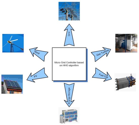
Figure 1.
Example of a microgrid with an energy management system (EMS) based on Harris hawk optimization (HHO) proposed in this paper.
The main role of the EMS is to decide the amount of energy that needs to be supplied by the DERs within the microgrid and to organize the power exchange between the unified grid and the microgrids. The decisions of the EMS are based on the ability of DERs and the current prices of energy. This means that the EMS must take accurate decisions to balance between increasing local production and maximizing economic revenue. Consequently, energy management of microgrids forms a highly constrained optimization problem and this optimization problem is usually considered an offline one [8].
From the above-mentioned explanation, it is clear that the EMS’s objective function depends on providing various types of data. Some of these data can be easily determined, such as the generation capacities of the grid and microturbines. However, most of them depend on forecasts and estimations such as loading limits, wind speed, solar irradiance, energy prices, etc. As a result, the researchers have followed two techniques in optimizing the EMS’s objective function [9,10].
The first is the deterministic approach: in this approach, all forecasted data are taken into consideration as they are assuming that they have very high accuracy. The other approach is the probabilistic approach in which all forecasted data are put in the form of variables. Each variable has a probability that resembles the accuracy of the forecast.
Researchers have applied many optimization algorithms to solve the EMS problem. One of the famous techniques is linear programming (LP) which considers the power balance and generation limits of the distributed generation units. However, this method suffers from one main disadvantage, which is a high computational burden [11,12,13].
One of the popular optimization techniques that have been incorporated in solving the EMS problem is dynamic programming (DP). The main advantage of this method is its ability to divide the EMS into smaller sub-problems. This means that the optimization technique will solve sequential problems instead of solving one sophisticated problem, which helps in reaching the optimum solution with quick and accurate performance. However, the operation of this algorithm is considered difficult since it includes a high number of recursive functions [14].
In [15], a genetic algorithm is used in optimizing the EMS’s objective function. This method has better computational burden when compared to LP. However, still the computational complexity exists.
Multi agent (MA) optimization has gained great researchers attraction in solving the EMS optimization problem. Although this method has relatively high accuracy considering many constrains, it suffers also from high computational complexity and time [16,17,18,19].
Particle swarm optimization (PSO) has attracted many researchers as well to use it in the optimization of the EMS problem. This method showed better results compared to previously mentioned methods in terms of accuracy and computational burden [15,20].
In [21], authors proposed the artificial bee colony (ABC) to solve the EMS problem. Although this method is considered quite simple and has robust performance, the formulation of the EMS problem to adapt between it and the algorithm is considered complex as this technique is suitable for objective functions that do not have high number of parameters.
This technique has directed many researchers to use various meta-heuristic optimization algorithms such as grey wolf optimization (GWO) [22], evolutionary algorithms (EA), etc.
Another research direction led by many researchers depends on coordinated control. In [23] a coordinated controller for a microgrid based on a predictive model and voltage control is presented. The main advantage of this method is that it needs less effort in the tuning of the controller. Authors of [24] also proposed a multi-layer coordinated control technique for the energy management of microgrids based on forecasting customer loading. Furthermore, another method of coordinated control is presented in [25]. This method depends on bi-level stochastic modelling.
Most of papers mentioned in literature have suffered from drawbacks (particularly in the modelling of the system) that can be summarized in the following points [11,12,15,21,22,26,27,28,29]:
- Power losses are not taken into considered in some papers.
- Battery charging and discharging intervals are not considered in some papers.
- High computational complexity in some of the above indicated references.
In this paper, the Harris hawk optimization (HHO) is used in solving the EMS optimization problem in a grid connected microgrids. The algorithm is applied to a highly constrained objective function which takes into consideration many important constraints such as power balance, generation power capacities, spinning reserve and energy storage limits (including charging and discharging rates). The proposed algorithm shows an improved performance compared to other algorithms used previously in literature in terms of speed of convergence and minimization of cost of operation when compared head-to-head and applied to same test bench. The proposed HHO algorithm may form a good optimization technique for solving other optimization problems in the power and energy fields.
The rest of this paper is organized as follows: Section 2 shows the problem formulation of the EMS optimization problem, while Section 3 explains the HHO algorithm and its application to the proposed EMS optimization algorithm. In Section 4 the results of applying the proposed EMS optimization algorithm to a real microgrid with two different operating scenarios are presented. In Section 5 and Section 6, respectively, the discussion and conclusion are presented for the evaluation of the effectiveness of the proposed EMS algorithm.
2. EMS Problem Formulation
The EMS problem is defined as minimizing the operational cost of the microgrid by means of adjusting the generation parameters of different DERs and the utility grid. The optimization problem also considers open market prices for energy received from the grid and DERs.
2.1. Objective Function
As mentioned before, the objective function of the EMS is to minimize the operation cost of the microgrid as shown in Equation (1):
where is the generated active power of the generator i at time t. is the power exchanged between the utility grid and the microgrid at time t. is the cost per kW of the active power generated by the ith DER. is the market price of active power exchanged between the utility grid and the local microgrid.
NT is the total hours included in the objective function which is usually a 24 h period and NG is the total number of distributed generation units including storage units.
2.2. Constraints of the Objective Function
To simulate the real response of a microgrid against the decisions of the EMS, it is essential to put many constraints that are mandatory for smooth operation of the microgrid.
The first constraint is that all active power generated by all DERs and the grid must equal the load active power as per Equation (2).
where is the value of the load active power at time t, ND is total number of load levels.
Additionally, it is important to include the generation limits for each DER and the utility grid as illustrated in Equations (3) and (4). These are mandatory to guarantee stable operation of the microgrid.
where and are the generating limits of the generator i at time t while and are the generating limits of the utility grid at time t.
To keep the system running with high reliability, it is essential to include a portion of the microgrid generation capacity as spinning reserve, especially if most of the DERs are from renewable resources that may suffer from output instability. Equation (5) describes how the criteria of spinning reserves are met.
where is the scheduled spinning reserve at time t.
One of the important constraints for energy storage elements is the limitation of charge and discharge cycles, especially the time interval needed for each cycle. The amount of energy stored in the battery is calculated based on the following rule:
where is the amount of energy stored in the battery. is the allowed rate of charge while is the allowed rate of discharge. is a predefined time period in which the rate of charge or discharge is allowed.
2.3. Calculation of Energy Cost and Bids for the Microgrid Elements
According to the EMS objective function mentioned in Equation (1), the main role of the EMS is to reduce the energy cost of the microgrid. Because of this, it is very important to calculate the energy cost of each source used in the microgrid and the energy price of the utility grid.
Regarding the fuel cell and the microturbine, the bid price is calculated according to (8):
where is the bid price in €/h and is the price of fuel in €/kW h. is the electrical output power in kW. is the efficiency of the generation unit. is the payback amount of the cost of investment of the generation unit which can be get from (9) as follows:
where is the nominal generation power of the generation unit. AP is the annual energy production in kW h/kW. AC is the annual investment cost which is based on the following rule:
where i is the interest rate, n is the depreciation period and is the installation cost.
3. Proposed HHO-Based EMS
Harris hawk optimization is a metaheuristic optimization which was proposed in [30], and its mathematical model is inspired from the cooperative behavior of Harris hawks in hunting, chasing and besieging their victims. The HHO is based on population optimization without having any gradients which gives it competitive edge over other techniques in terms of speed of conversion.
The HHO consists of two main phases: exploration and exploitation. Additionally, there is a transition phase though which the algorithm is switched from exploration to exploitation.
In the exploration phase, Harris hawks start to search randomly for victims as per the following equation:
where is the location of the hawks in the iteration , is the location of the rabbit (the victim), to and are random numbers that can vary between 0 and 1, represents a hawk which is chosen randomly and is the average location of the current population of hawks which can be calculated from Equation (12):
where indicates the position of each hawk at iteration t while N represents the total number of hawks.
As mentioned above, after finishing the exploration stage, there is a transient stage before moving to the exploitation stage. At this transient stage, it is necessary to model the energy of the rabbit as per Equation (13):
where E is the escaping energy of the rabbit, T is the maximum number of iterations and is the initial state of the rabbit energy. The value of is varying between −1 and 1 based on the physical fitness of the victim. When goes towards −1, this means that the victim is losing its energy and vice versa.
According to the behavior of rabbits, the relation between the rabbit energy and the time is inversely proportional. This means that as long as increases, the is decreased. Based on , Harris hawks also decide to either search different areas to detect the location of the rabbit when or move forward to the exploitation phase.
In the exploitation phase, there are two behaviors that need to be modelled. The first is the soft besiege in which the rabbit energy is still high and can run fast; in this condition Harris hawks try to softly follow and put it under surveillance until it starts to get exhausted. The second behavior is the hard besiege; the prey in this behavior is tired and has no sufficient energy to escape. As a result, the Harris hawks in this mode form closed circles to make a sudden attack. Figure 2 shows Harris hawk attack patterns.
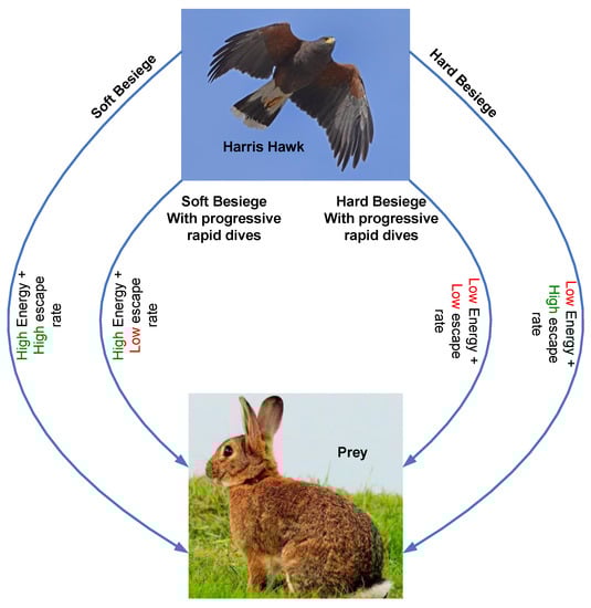
Figure 2.
Harris hawk prey attack patterns.
To mathematically model the two behaviors, let be the percentage of the successful escape of the rabbit. If and , this means that the rabbit has relatively high escaping energy and at the same time the chance of successful escape is higher than 50%. This means that the Harris hawks will perform a soft besiege and will update their location according to Equation (14):
where is the position difference between the rabbit and the hawks. This value can be calculated as follows:
where is a random number that represents the jump strength that can be met from Equation (16) as follows:
where is a random number that varies between 0 and 1.
If and , this means that the rabbit has high energy. However, the chance of successfully escaping is not big. In this case, the Harris hawks will perform a soft besiege but with progressive and rapid dives. The next movement of the hawks will be updated according to:
The hawks then will compare the current position with the previous dive to evaluate which is better. If the previous dive is better, the hawks will use it. If not, the hawks will then apply new dive using the levy flight (LF) equation:
where D is the problem dimension and S is a random vector with size of 1 × D. The LF function can be calculated according to (19) as noted in [31]:
where u and v are random numbers that vary between 0 and 1. is a constant value of 1.5. is calculated using:
The Harris hawks will then evaluate the positions Y and Z and then select the best position based on (21):
where only the better location of either Y or Z will be used to update the hawk’s position.
If and , this means that the rabbit has relatively low energy but it has a moderate chance of a successful escape. In this condition, the hawks will perform a hard besiege and will update their equation based on Equation (22):
If and , this means that the victim has low energy and also has a low chance to escape. In this situation, the hawks will also perform a hard besiege but with progressive rapid dives at which the next position of the hawks will be updated using Equation (21). Z will be calculated from Equation (18) and Y will be calculated using Equation (23) as follows:
The proposed EMS uses the HHO in evaluating the optimum values for generated powers from different DGs within the microgrid. The HHO in this optimization problem will consider the DG-generated powers as the location of the Harris hawks and the prey will represent the energy cost. Figure 3 shows a flowchart of the proposed HHO algorithm while Figure 4 shows a flowchart for the proposed EMS algorithm.
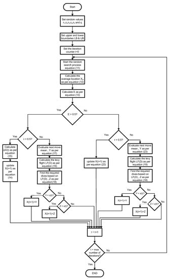
Figure 3.
HHO algorithm flowchart.
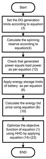
Figure 4.
The flowchart of the proposed EMS.
4. Simulation Results
To validate the effectiveness of the proposed algorithm, a microgrid is simulated using MATLAB. The output power of its DG units and grid is set by the proposed EMS. The simulated microgrid consists of PV, WT, DEG, FC, battery storage and a connection to the utility grid. This benchmark has been used by previous research [31] and has been chosen to be simulated in this paper in order to be able to compare obtained results with previous research results available in literature. Table 1 shows the minimum and maximum output power of each element of the microgrid as well as coefficients of bid functions, where the negative sign indicates direction of power flow. Table 2 presents sample forecast values for the load demand and DG units’ powers along with market price. Two case studies are simulated to evaluate the effectiveness of the proposed HHO-based EMS on different operating conditions. Cost is expressed in units of euro cents (€ ct).

Table 1.
Power limits and coefficients of bid functions of the installed distributed generation (DG) units.
Table 2.
The forecast values of load demand, market price, wind and photovoltaic (PV) power production.
4.1. Case Study 1
In this case, the PV and WT will supply their maximum available generating power according to the hourly forecast. The proposed EMS controls and sets the output power of the other DG units to decrease the generating cost and according to their corresponding power limits and constraints.
The results of the proposed algorithm are tabulated in Table 3. When observing the behavior of the proposed EMS during the first and last eight hours of the day, results show that during these periods the proposed EMS depends on the FC and the utility grid for generating the largest portion of output power. This occurs because the energy price during these periods is low which means that generating electricity from the utility grid is cheaper than the DEGs. This is not the case at midday, when the EMS mainly depends on the PV, WT and DEG units as the energy price of the utility grid is expensive.
Table 3.
Results of Case Study 1.
4.2. Case Study 2
In this case, the output power of all DG units including PV and WT are controlled by the EMS within their constrains and power limits. The results of this case, which are shown in Table 4, show a huge reduction in the total cost of energy compared to that of case 1. The reason for this is that the EMS fully controls DG units aiming to reduce the total cost. This leads to higher dependency on the utility grid during low energy bids.
Table 4.
The best solutions obtained for solving EOM problem for Case Study 2.
Results of both cases show the HHO algorithm functions properly during different modes of operation for the EMS. Figure 5, which indicates the conversion curve sample of the HHO algorithm, clearly shows the effectiveness of the proposed method as the conversion rate is fast during both cases.
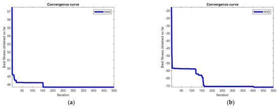
Figure 5.
Convergence curves for the HHO algorithm for (a) Study Case 1 sample, (b) Study Case 2 sample.
5. Discussion and Analysis
In order to validate the obtained results confidently, it is important to compare the results of HHO algorithm in both cases with earlier research results that used the exact microgrid simulation model but with different optimization algorithms, such as fast surrogate-assisted particle swarm optimization (FSAPSO) and several modified PSO algorithms [31]. Table 5 shows the obtained results of the HHO algorithm along with results of other previously proposed algorithms in literature. Number of objective function evaluations (OFE) carried out till best solution is reached is indicated where it is equal to 1× number of agents × iterations. Additionally, the number of algorithm iterations needed till best solution is reached is indicated in the table along the trials number. Although there is a lack in information in [31], it can be noted that the proposed HHO algorithm successfully reaches lower operating costs with lower iterations. It is suggested as future work to take into consideration other constraints such as PV lifetime and power degradation, and battery state of health and power degradation, where some modifications can be made to power constraints, mentioned earlier in Table 1, accordingly, to give more realistic results especially for long term simulations.
Table 5.
Comparison of the obtained simulation results for the MG—Case 1 & 2 [31].
6. Conclusions
Power generation cost optimization is considered one of the main problems facing modern microgrids having different energy resources and interconnections. In this paper, the generation cost optimization problem with all its constraints is explained in detail. A new optimization technique, Harris hawk optimization, is presented thoroughly as a proposed solution to the energy management optimization problem. The proposed algorithm is tested using MATLAB simulation on a benchmark microgrid and results are compared with previous research. The Harris hawk algorithm succeeded in achieving much-improved results as it produced the lowest generation cost in comparison with other widely used optimization algorithms. Obtained results indicate that the Harris hawk algorithm should be tested further on other applications in the field of power and energy management as it may form a strong and reliable computation algorithm.
Author Contributions
M.A. contributed to the research framework, checked, and revised draft paper; H.Y.D. collected the data and wrote the draft manuscript, checked, and revised the paper; A.A.E.-B. supervised the whole process. All authors have read and agreed to the published version of the manuscript.
Funding
This research received no external funding.
Conflicts of Interest
The authors declare no conflict of interest.
Nomenclature
The following symbols are used in this manuscript:
| minimum operation cost | |
| cost per kW of active power generated by i | |
| generated active power of i | |
| t | time |
| power exchange between utility grid and microgrid | |
| market price of active power exchanged | |
| NT | total hours |
| NG | total number of distributed generations |
| ND | total number of load levels |
| MG | Microgrid |
| load active power at time t | |
| minimum generation limit of generator i at time t | |
| maximum generation limit of generator i at time t | |
| minimum generation limit of utility grid at time t | |
| maximum generation limit of utility grid at time t | |
| cheduled spinning reserve at time t | |
| energy stored in battery | |
| minimum energy to be stored in battery | |
| maximum energy to be stored in battery | |
| rate of charge | |
| rate of discharge | |
| max charge | |
| max discharge | |
| predefined time for charge or discharge | |
| charge efficiency | |
| discharge efficiency | |
| bid price | |
| price of fuel | |
| output power | |
| generation unit efficiency | |
| payback amount | |
| nominal power generation | |
| bid price | |
| AP | annual energy production |
| annual investment cost | |
| installation cost | |
| location of hawk at iteration t+1 | |
| location of rabbit | |
| random choice of hawk | |
| average location of current population of hawks | |
| position of hawk i at iteration t | |
| total number of hawks | |
| escaping energy of rabbit | |
| initial energy of rabbit | |
| maximum number if iterations | |
| r | percentage of successful rabbit escape |
| position difference between rabbit and hawks | |
| jump strength | |
| random numbers between 0 and 1 | |
| LF | levy flight |
| Y, Z | next movement update |
| problem dimension | |
| S | random vector with size 1 × D |
| u, v | levy flight random value between 0 and 1 |
| constant of value 1.5 |
References
- Renewables. International Energy Agency, IEA. 2019. Available online: https://www.iea.org/topics/renewables/ (accessed on 30 September 2020).
- Parhizi, S.; Lotfi, H.; Khodaei, A.; Bahramirad, S. State of the art in research on microgrids: A review. IEEE Access 2015, 3, 890–925. [Google Scholar] [CrossRef]
- Lasseter, R.H. MicroGrids. In Proceedings of the 2002 IEEE Power Engineering Society Winter Meeting, New York, NY, USA, 27–31 January 2002; pp. 305–308. [Google Scholar]
- Afgan, N.H.; Carvalho, M.G. Sustainability assessment of a hybrid energy system. Energy Policy 2008, 36, 2903–2910. [Google Scholar] [CrossRef]
- Hatziargyriou, N.; Asano, H.; Iravani, R.; Marnay, C. Microgrids: An Overview of Ongoing Research, Development, and Demonstration Projects. IEEE Power Energy 2007, 5, 78–94. [Google Scholar] [CrossRef]
- Lasseter, R.H. CERTS Microgrid. In Proceedings of the 2007 IEEE International Conference on System of Systems Engineering, San Antonio, TX, USA, 16–18 April 2007. [Google Scholar]
- Stanton, K.N.; Giri, J.C.; Bose, A. Energy management. In Systems, Controls, Embedded Systems, Energy, and Machines; CRC Press: Boca Raton, FL, USA, 2017. [Google Scholar]
- Shi, W.; Li, N.; Chu, C.C.; Gadh, R. Real-Time Energy Management in Microgrids. IEEE Trans. Smart Grid 2017, 8, 228–238. [Google Scholar] [CrossRef]
- Su, W.; Wang, J. Energy Management Systems in Microgrid Operations. Electr. J. 2012, 25, 45–60. [Google Scholar] [CrossRef]
- Gildardo Gómez, W.D. Metodología para la Gestión Óptima de Energía en una Micro red Eléctrica Interconectada. Ph.D. Thesis, Universidad Nacional de Colombia, Medellín, Colombia, 2016. [Google Scholar]
- Taha, M.S.; Mohamed, Y.A.R.I. Robust MPC-based energy management system of a hybrid energy source for remote communities. In Proceedings of the 2016 IEEE Electrical Power and Energy Conference (EPEC), Ottawa, ON, Canada, 12–14 October 2016. [Google Scholar]
- Sukumar, S.; Mokhlis, H.; Mekhilef, S.; Naidu, K.; Karimi, M. Mix-mode energy management strategy and battery sizing for economic operation of grid-tied microgrid. Energy 2017, 118, 1322–1333. [Google Scholar] [CrossRef]
- Delgado, C.; Dominguez-Navarro, J.A. Optimal design of a hybrid renewable energy system. In Proceedings of the 2014 Ninth International Conference on Ecological Vehicles and Renewable Energies (EVER), Monte-Carlo, Monaco, 25–27 March 2014. [Google Scholar]
- Wu, N.; Wang, H. Deep learning adaptive dynamic programming for real time energy management and control strategy of micro-grid. J. Clean. Prod. 2018, 204, 1169–1177. [Google Scholar] [CrossRef]
- Li, H.; Eseye, A.T.; Zhang, J.; Zheng, D. Optimal energy management for industrial microgrids with high-penetration renewables. Prot. Control Mod. Power Syst. 2017, 2, 1–14. [Google Scholar] [CrossRef]
- Anvari-Moghaddam, A.; Rahimi-Kian, A.; Mirian, M.S.; Guerrero, J.M. A multi-agent based energy management solution for integrated buildings and microgrid system. Appl. Energy 2017, 203, 41–56. [Google Scholar] [CrossRef]
- Kumar Nunna, H.S.V.S.; Doolla, S. Energy management in microgrids using demand response and distributed storage—A multiagent approach. IEEE Trans. Power Deliv. 2013, 28, 939–947. [Google Scholar] [CrossRef]
- Dou, C.X.; Liu, B. Multi-agent based hierarchical hybrid control for smart microgrid. IEEE Trans. Smart Grid 2013, 4, 771–778. [Google Scholar] [CrossRef]
- Karavas, C.S.; Kyriakarakos, G.; Arvanitis, K.G.; Papadakis, G. A multi-agent decentralized energy management system based on distributed intelligence for the design and control of autonomous polygeneration microgrids. Energy Convers. Manag. 2015, 103, 166–179. [Google Scholar] [CrossRef]
- Azaza, M.; Wallin, F. Multi objective particle swarm optimization of hybrid micro-grid system: A case study in Sweden. Energy 2017, 123, 108–118. [Google Scholar] [CrossRef]
- Marzband, M.; Azarinejadian, F.; Savaghebi, M.; Guerrero, J.M. An optimal energy management system for islanded microgrids based on multiperiod artificial bee colony combined with markov chain. IEEE Syst. J. 2015, 11, 1712–1722. [Google Scholar] [CrossRef]
- Ei-Bidairi, K.S.; Nguyen, H.D.; Jayasinghe, S.D.G.; Mahmoud, T.S. Multiobjective Intelligent Energy Management Optimization for Grid-Connected Microgrids. In Proceedings of the 2018 IEEE International Conference on Environment and Electrical Engineering and 2018 IEEE Industrial and Commercial Power Systems Europe (EEEIC/I&CPS Europe), Palermo, Italy, 12–15 June 2018. [Google Scholar]
- Hu, J.; Shan, Y.; Xu, Y.; Guerrero, J.M. A coordinated control of hybrid ac/dc microgrids with PV-wind-battery under variable generation and load conditions. Int. J. Electr. Power Energy Syst. 2019, 104, 583–592. [Google Scholar] [CrossRef]
- Mahmud, K.; Sahoo, A.K.; Ravishankar, J.; Dong, Z.Y. Coordinated multilayer control for energy management of grid-connected AC microgrids. IEEE Trans. Ind. Appl. 2019, 55, 7071–7081. [Google Scholar] [CrossRef]
- Wang, Z.; Chen, B.; Wang, J.; Begovic, M.M.; Chen, C. Coordinated energy management of networked microgrids in distribution systems. IEEE Trans. Smart Grid 2014, 6, 45–53. [Google Scholar] [CrossRef]
- Helal, S.A.; Najee, R.J.; Hanna, M.O.; Shaaban, M.F.; Osman, A.H.; Hassan, M.S. An energy management system for hybrid microgrids in remote communities. In Proceedings of the 2017 IEEE 30th Canadian Conference on Electrical and Computer Engineering (CCECE), Windsor, ON, Canada, 30 April–3 May 2017. [Google Scholar]
- Chaouachi, A.; Kamel, R.M.; Andoulsi, R.; Nagasaka, K. Multiobjective intelligent energy management for a microgrid. IEEE Trans. Ind. Electron. 2013, 60, 1688–1699. [Google Scholar] [CrossRef]
- Abedini, M.; Moradi, M.H.; Hosseinian, S.M. Optimal management of microgrids including renewable energy scources using GPSO-GM algorithm. Renew. Energy 2016, 90, 430–439. [Google Scholar] [CrossRef]
- Wasilewski, J. Optimisation of multicarrier microgrid layout using selected metaheuristics. Int. J. Electr. Power Energy Syst. 2018, 99, 246–260. [Google Scholar] [CrossRef]
- Heidari, A.A.; Mirjalili, S.; Faris, H.; Aljarah, I.; Mafarja, M.; Chen, H. Harris hawks optimization: Algorithm and applications. Future Gener. Comput. Syst. 2019, 97, 849–872. [Google Scholar] [CrossRef]
- Anvari-Moghaddam, A.; Seifi, A.; Niknam, T.; Pahlavani, M.A. Multi-objective Operation Management of a Renewable Micro Grid with Back-up Micro Turbine/Fuel Cell/Battery Hybrid Power Source. Energy Int. J. 2011, 36, 6490–6507. [Google Scholar] [CrossRef]


Publisher’s Note: MDPI stays neutral with regard to jurisdictional claims in published maps and institutional affiliations. |
© 2021 by the authors. Licensee MDPI, Basel, Switzerland. This article is an open access article distributed under the terms and conditions of the Creative Commons Attribution (CC BY) license (https://creativecommons.org/licenses/by/4.0/).