Article

Kinetic Analysis Misinterpretations Due to the Occurrence of Enzyme Inhibition by Reaction Product: Comparison between Initial Velocities and Reaction Time Course Methodologies

by
Joana M. C. Fernandes
1,
Albino A. Dias
1,2 and
Rui M. F. Bezerra
1,2,*
1
CITAB—Centre for the Research and Technology of Agro-Environmental and Biological Sciences, UTAD—Universidade de Trás-os-Montes e Alto Douro, 5000-801 Vila Real, Portugal
2
Department of Biology and Environment, UTAD—Universidade de Trás-os-Montes e Alto Douro, 5000-801 Vila Real, Portugal
*
Author to whom correspondence should be addressed.
Appl. Sci. 2022, 12(1), 102; https://doi.org/10.3390/app12010102
Submission received: 21 October 2021 / Revised: 30 November 2021 / Accepted: 21 December 2021 / Published: 23 December 2021
(This article belongs to the Special Issue Enzyme Catalysis: Advances, Techniques, and Outlooks)

Abstract

:

Featured Application

The integrated Michaelis–Menten equation (IMME) provides a viable and accurate methodology for enzyme kinetic studies when the product is also an inhibitor. This methodology is important in a wide range of applications, including in the preclinical kinetic assays of potential drug candidates. This methodology is a powerful tool for overcoming the inaccuracies associated with archaic curve linearization methods for initial velocities determination mainly when the reaction product is an enzyme inhibitor.

Abstract

The Michaelis–Menten equation (MME) has been extensively used in biochemical reactions, but it is not appropriate when the reaction product inhibits the enzyme. Under these circumstances, each determined initial velocity, v0, is one experimental point that actually belongs to a different MME because enzymatic product inhibition occurs as the reaction starts. Furthermore, the inhibition effect is not constant, since the concentration of the product inhibitor rises as time increases. To unveil the hidden enzyme inhibition and to simultaneously demonstrate the superiority of an integrated Michaelis–Menten equation (IMME), the same range of data points, assuming product inhibition and the presence of a second different inhibitor, was used for kinetic analysis with both methodologies. This study highlights the superiority of the IMME methodology for when the enzyme is inhibited by the reaction product, giving a more coherent inhibition model and more accurate kinetic constants than the classical MME methodology.

1. Introduction

Enzymes are catalysts with diverse substrate specificities that have been used to modulate biochemical transformations and which play an important role in a wide range of applications, including proteomics research, medical diagnosis, food processing, biofuel production, and environmental monitoring [1]. Furthermore, studies of enzyme kinetics with more than one inhibitor have been specially focused in the pharmaceutical industry on the development of more effective drugs that act at signal transduction cascades and metabolic pathway levels [2].
At the beginning of the 20th century, Henri [3] proposed the first mathematical formulation for enzymatic kinetics, corresponding to an equation that represented product versus time. Slightly later (1913), Michaelis and Menten made a proposal based on an equation of initial velocity versus substrate concentration using the catalytic constant (kcat) and a substrate constant (Ks ≈ Km) [4], which has been the basis of the great majority of kinetic studies carried out until today. However, from a formal point of view, the occurrence of enzyme inhibition via a reaction product was not considered in this equation. This fact deserves special attention, since it has been reported that 91.7% of human enzymes exhibit inhibition and the most inhibitory interactions result from the structural similarities between substrates and inhibitors [5]. This emphasizes the extreme importance of product inhibition in kinetic studies. Since product inhibition can significantly retard the rates of enzyme-catalyzed reactions [6], the accumulated product constitutes the main obstacle for the determination of the true initial velocities using conventional assay methods [7].
When the reaction product inhibits the enzyme, the obtained initial velocity points adjust to the Michaelis–Menten equation (MME), and are always affected by the inhibitor’s action [8,9]. However, kinetic studies under these conditions are usually performed by adjusting the initial velocities to an MME (without considering the effect of the inhibitor’s presence). However, if the product is an inhibitor, the initial velocity determined cannot be the “true” initial velocity without the inhibitor, because the inhibitor (a reaction product) has been there since the reaction started. Thus, the utilization of an appropriate integrated Michaelis–Menten equation (IMME) provides a viable and unique methodology that can overcome such limitations. Nevertheless, before parameter estimation, model discrimination is required as a first step in order to find an IMME model that best fits the experimental points. Actually, the use of integrated equations to study enzyme kinetics is no longer a complex task since the required nonlinear regression methods are available in software spreadsheets using traditional widespread desktop tools, such as Office Excel [8,9,10,11,12].
The main aim of this work is to present and validate a methodology based on an IMME (with different inhibitor models) that is capable of overcoming the misinterpretations that arise when using usual initial velocities methodology [13] when an enzyme is inhibited by the reaction product. Both methodologies (MME and IMME) were used with same simulated data points (product vs. time) and the results were compared in order to find the best one.

2. Materials and Methods

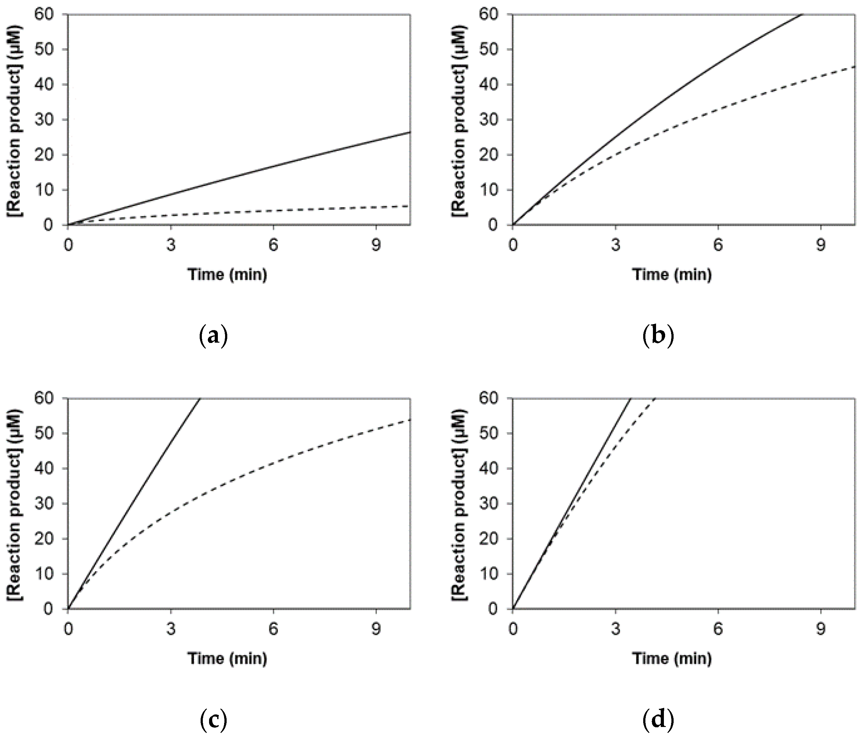
2.1. Simulated Data for the Graphical Representation of Product Versus Time

Simulated data representing product versus time curves with integrated equations considering the absence of product inhibition (Equation (1), Table 1 and Figure 1a) and also competitive inhibition by the reaction product (Equation (2), Table 1 and Figure 1b) were used to obtain four graphical representations of different Km/Ki (Figure 2). The following arbitrary parameters were used in the simulation: (a) Vmax = 18 μM min−1; Km = 500 μM; S0 = 100 μM; Kic = 0.5 μM; (b) Vmax = 18.0 μM min−1; Km = 100 μM; S0 = 100 μM; Kic = 20 μM; (c) Vmax = 18.0 μM min−1; Km = 10 μM; S0 = 100 μM; Kic = 2 μM. (d) Vmax = 18.0 μM min−1; Km = 2 μM; S0 = 100 μM; Kic = 5 μM.

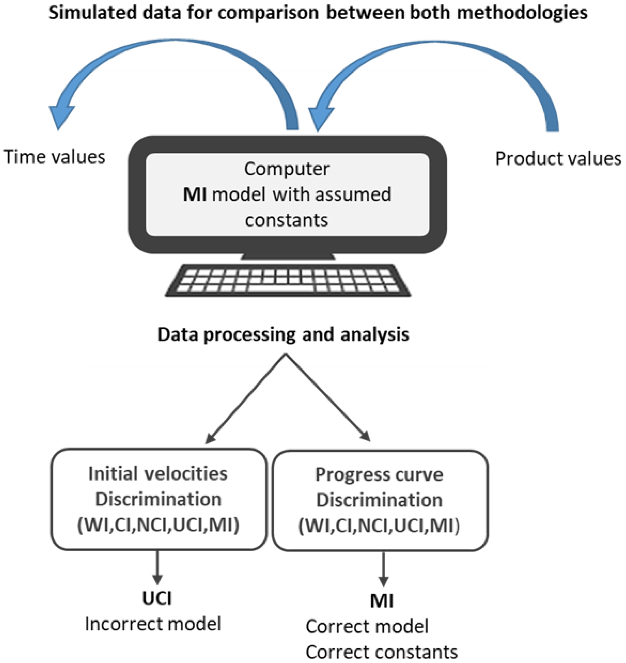
2.2. Simulated Data for Comparison between Both Methodologies

Simulated data points [P] vs. time were obtained, taking into account the presence of mixed inhibition by the reaction product [I1] and furthermore the presence of a second different mixed inhibitor, [I2] = 10 μM (Table 2, Equation (9), two mixed mutually exclusive inhibitors). Data points were simulated with the following arbitrary kinetic parameters: (Km = 500 μM; Vmax = 0.120 μmol min−1 mg−1; Kic1 = 100 μM; Kiu1 = 50 μM; Kic2 = 50 μM; Kiu2 = 5 μM) at six substrate concentrations (100; 200; 400; 800; 1000; 2000 μM).
Only data points in the “linear” part of each curve [P] vs. time were used for subsequent kinetic analysis [10,12].

2.3. Data Processing and Analysis

Based on the same set of simulated values, obtained as explained in Section 2.2, conventional kinetics based on the initial velocities (MME) was performed similarly to a previously published work [13]. The same data points were also submitted to a kinetic analysis using integrated equations (IMME) [8,10], assuming the presence of two inhibitors (mutually exclusive when one of which is a reaction product) and considering the following models: MI model (Equation (9)); UCI (Equation (8)); NCI (Equation (7)); CI (Equation (6)); and WI (Equation (1)).
The estimation of kinetic constants was carried out through the nonlinear regression of the experimental data using the Solver supplement of Microsoft Office Excel [13]. The discrimination between different kinetic models was performed using the Akaike information criterion (AIC) [8,14], as previously explained. Kinetic parameter uncertainties were determined using the sequential quadratic programming algorithm from SPSS Statistics 23 (IBM, Armonk, NY, USA) software.

3. Results

3.1. Simulated Data for the Graphical Representation of Product Versus Time

Assuming the kinetic inhibition by the reaction product (Figure 1a) or considering the simultaneous presence of two mutually exclusive inhibitors when one of which is a reaction product (Figure 1b), this work intends to highlight possible inaccuracies when kinetic studies are carried out using conventional methodologies (initial velocities) [13]. The integrated equations with one inhibitor (Figure 1a) are presented in Table 1. Model MI (Equation (5)) can be simplified into other nested models with fewer parameters (Table 1), assuming that constants Kic and Kiu both tend to infinity (WI, Equation (1)), that only one of them does (CI, Kiu → ∞, Equation (2) or UCI, Kic → ∞, Equation (4)), or that both are equal (NCI, Kic = Kiu, Equation (3)).
To clarify the need for a new approach to the study of enzyme kinetics when reaction product inhibition occurs, a simulation (Figure 2) was carried out using integrated equations (Table 1) considering the absence of product inhibition (Equation (1)) and admitting, e.g., that the reaction product is a competitive inhibitor (Equation (2)).

3.2. Kinetic Studies Using MME and IMME Based on Simulated Values

When reactions are carried out in the presence of a second inhibitor, another set of integrated equations assumes the simultaneous presence of two mutually exclusive inhibitors (Figure 1b), where one of which is a reaction product. This process is presented in Table 2 [8]. In the presence of two inhibitors, a linear MI model (Equation (9), Table 2) can be simplified into other nested models with fewer parameters (Equations (1), (6)–(8), assuming that constants Kic1, Kic2, Kiu1, Kiu2 tend to infinity (WI, Equation (1)) or only some of them do (CI or UCI, (Equations (6) and (8)), or when Kic1 = Kiu1 and Kic2 = Kiu2 (NCI, Equation (7)).
The initial velocities obtained with the theoretically simulated data points without or with a second inhibitor were used for the kinetic investigation using a conventional MME. Discrimination among the different kinetic models (Table 3,) using AIC methodology can be seen in Table 4. Uncompetitive inhibition (MME) was discriminated as the best fit model and the estimated parameters are presented in Table 5. The same discrimination methodology for the different IMME models (Table 3) shows that the best model is the MI model (Equation (9)). In addition to discriminating between different models (UCI and MI, respectively, by the MME and IMME methodologies), the results show notable differences between the values of the kinetic parameters determined for both models (Table 5).

4. Discussion

As can be seen in Figure 2, the experimental points for product versus time cannot be the same once the equations are different. The ratios for Km/Kic were 1000, 5, 5 and 0.4, respectively to Figure 2a–d. In Figure 2a,b the enzyme is not in saturated conditions, unlike what happens in Figure 2c,d. The kinetic constant Kic (product inhibitor) used to obtain the different curves for Figure 2a is much smaller than Km. Even when Km and Kic have the same order of magnitude (Figure 2b,c) or Kic is greater than Km (Figure 2d), the initial velocities with and without the inhibitor seem similar, but are not the same, as previously discussed [10,12]. In traditional enzyme kinetics lab work, experimental data is usually forced to be adjusted to the Michaelis–Menten equation, i.e., uninhibited conditions are assumed. However, as Figure 2 shows, the initial velocities determined from the derivatives (tangents) of Equation (1) (solid line, without inhibition by the reaction product) and Equation (2) (dashed line, competitive inhibition by the reaction product) at time zero are different mainly when the Km/Kic ratio is greater than 1 (Figure 2a–c). Therefore, if product inhibition occurs, the initial velocity can never be an experimental point of the Michaelis–Menten equation (v0 = Vmax [S]/(Km + [S]) as assumed by the initial velocities methodology. Unfortunately, all published kinetic studies that use the initial velocities methodology when the product is an inhibitor have this evident incompatibility. Thus, initial velocity studies in the presence of reaction product inhibition have two implicit drawbacks: (1) the initial velocities of these two equations (without product inhibition and with product inhibition) are the same; and (2) it is assumed that the initial velocities are data points belonging to the Michaelis–Menten equation (v0 = Vmax [S]/(Km + [S]). These methodological simplifications were overlooked about 100 years ago when it was very difficult to overcome these problems due to the lack of computers. Even after computer use became common, the determination of initial velocities when the product of the reaction is an inhibitor remains very popular.
In kinetic studies, equations must be adjusted to the data points prior to the discrimination of the best model. Unfortunately, in almost all published studies, data points were adjusted to the equations that were previously assumed to be correct. Thus, miscalculation begins with the initial velocity determinations when the reaction product inhibition is not considered [15,16]. The error can even be accentuated when, in many cases, the data points are adjusted to a particular inhibition model without considering other types of inhibition, which may provide better adjustments (e.g., non-competitive versus mixed inhibition). Inaccuracies are also amplified when the kinetics are studied using archaic curve linearization, such as with the popular Lineweaver–Burk plot, which is still used today [17], or other similar processes. The advantages of integrated equations have been presented by many authors and summarized in previous publications [8,9,10,12,18,19,20]. To emphasize the importance of this subject, misinterpretations can be increased when another different inhibitor is added to the reaction medium, which is a mandatory condition in kinetic inhibition studies [8,9]. A summary of the work carried out can be seen in the scheme presented in Figure 3.
To exemplify the errors obtained when the initial velocity is assumed, theoretical values (same data points, product versus time) were obtained with Equation (9) (Table 2) and the arbitrary values of the product (P) introduced in the equation (assuming predefined kinetics parameters) in order to obtain time (t) values (Km = 500 μM; Vmax = 0.120 μmol min−1 mg−1; Kic1 = 100 μM; Kiu1 = 50 μM; Kic2 = 50 μM; Kiu2 = 5 μM). It should be pointed out that ratios Km/Kic1 = 5 and Km/Kiu1 = 10 are in the same order of magnitude of simulations presented in Figure 2b,c. Moreover, these ratios are in the same order of magnitude exhibited by enzymes with product inhibition [10,11,21]. With these theoretical data points (product vs. time), the study was carried out using the initial velocity methodology (MME) and compared with an IMME based on the same data range (linear phase of product vs. time), i.e., using the same simulated points. The best methodology (MME or IMME) will be the one that provides similar kinetic parameters with those utilised for initial data point generation. As can be seen, the different values for the kinetic parameters and the inhibition model thus discriminated (UCI/MME) do not match the initial constants used to obtain the values of the data set (product vs. time). The kinetic constants obtained by the MME methodology were: Km = 344.4 μM instead of 500 μM; Vmax = 0.077 μmol min−1 mg−1 instead of 0.120 μmol min−1 mg−1; Kic2 = ∞ instead of 50 μM; and Kiu2 = 7.3 μM instead of 5 μM. On the contrary, the IMME methodology allowed us to obtain identical kinetic parameters (Table 5) and a kinetic model (MI) chosen to generate simulated data points (product vs. time). It is evident that the MME methodology (initial velocity) cannot be used to obtain Kic1 and Kiu1. In addition, this methodology also failed to discriminate the inhibition model for the second inhibitor (UCI instead of MI) and gave the kinetic parameters (Table 5) Km and Vmax with values lower than around 30%. These results highlight the superiority of the IMME methodology.

5. Conclusions

The kinetic analysis of enzymatic reactions in the presence of product inhibition gives different kinetic models as a function of the chosen methodology (initial velocities and progress curve analysis). The results obtained with the MME methodology (initial velocities) gives an inhibition model and parameter constants that do not match with the correct one. In contrast, the IMME methodology allowed us to obtain the same model (MI) and constants similar to the original ones used to obtain the initial data points.
Theoretical considerations regarding the use of integrated Michaelis–Menten equations to study enzyme kinetics when the reaction product is an enzyme inhibitor emphasize the superiority of the IMME approach over the classical MME methodology. Thus, kinetic studies, when the reaction product is an enzyme inhibitor, should be carried out using the IMME methodology in order to obtain the appropriate kinetic model and unbiased kinetic constants.

Author Contributions

Conceptualization, R.M.F.B. and A.A.D.; methodology, R.M.F.B. and A.A.D.; formal analysis, J.M.C.F.; investigation, J.M.C.F.; resources, R.M.F.B., and A.A.D.; writing—original draft preparation, J.M.C.F.; writing—review and editing, J.M.C.F., R.M.F.B. and A.A.D.; supervision, R.M.F.B. and A.A.D. All authors have read and agreed to the published version of the manuscript.

Funding

This work was supported by the National Funds of the FCT—Portuguese Foundation for Science and Technology, under the project UIDB/04033/2020.

Data Availability Statement

Data are available upon request to the authors.

Conflicts of Interest

The authors declare no conflict of interest.

References

  1. Adrio, J.L.; Demain, A.L. Microbial enzymes: Tools for biotechnological processes. Biomolecules 2014, 4, 117–139. [Google Scholar] [CrossRef] [Green Version]
  2. El Harrad, L.; Bourais, I.; Mohammadi, H.; Amine, A. Recent advances in electrochemical biosensors based on enzyme inhibition for clinical and pharmaceutical applications. Sensors 2018, 18, 164. [Google Scholar] [CrossRef] [Green Version]
  3. Henri, V. Theorie generale de l’action de quelques diástases. Comptes Rendus Biol. 1902, 135, 916–919. [Google Scholar]
  4. Michaelis, L.; Menten, M. Die kinetik der invertinwirkung. Biochem. Z. 1913, 49, 333–369. [Google Scholar]
  5. Alam, M.T.; Olin-Sandoval, V.; Stincone, A.; Keller, M.A.; Zelezniak, A.; Luisi, B.F.; Ralser, M. The self-inhibitory nature of metabolic networks and its alleviation through compartmentalization. Nat. Commun. 2017, 8, 16018. [Google Scholar] [CrossRef] [PubMed]
  6. Andrić, P.; Meyer, A.S.; Jensen, P.A.; Dam-Johansen, K. Reactor design for minimizing product inhibition during enzymatic lignocellulose hydrolysis: II. Quantification of inhibition and suitability of membrane reactors. Biotechnol. Adv. 2010, 28, 407–425. [Google Scholar] [CrossRef] [PubMed]
  7. Schmidt, N.D.; Peschon, J.J.; Segel, I.H. Kinetics of enzymes subject to very strong product inhibition: Analysis using simplified integrated rate equations and average velocities. J. Theor. Biol. 1983, 100, 597–611. [Google Scholar] [CrossRef]
  8. Bezerra, R.M.; Pinto, P.A.; Fraga, I.; Dias, A.A. Enzyme inhibition studies by integrated Michaelis–Menten equation considering simultaneous presence of two inhibitors when one of them is a reaction product. Comput. Meth. Prog. Biomed. 2016, 125, 2–7. [Google Scholar] [CrossRef]
  9. Bezerra, R.M.F.; Pinto, P.A.; Dias, A.A. A kinetic process to determine the interaction type between two compounds, one of which is a reaction product, using alkaline phosphatase inhibition as a case study. Appl. Biochem. Biotechnol. 2020, 191, 657–665. [Google Scholar] [CrossRef]
  10. Bezerra, R.M.; Fraga, I.; Dias, A.A. Utilization of integrated Michaelis-Menten equations for enzyme inhibition diagnosis and determination of kinetic constants using Solver supplement of Microsoft Office Excel. Comput. Meth. Prog. Biomed. 2013, 109, 26–31. [Google Scholar] [CrossRef] [PubMed]
  11. Bezerra, R.M.; Dias, A.A.; Fraga, I.; Pereira, A.N. Simultaneous ethanol and cellobiose inhibition of cellulose hydrolysis studied with integrated equations assuming constant or variable substrate concentration. Appl. Biochem. Biotechnol. 2006, 134, 27–38. [Google Scholar] [CrossRef]
  12. Bezerra, R.M.; Dias, A.A. Utilization of integrated Michaelis-Menten equation to determine kinetic constants. Biochem. Mol. Biol. Educ. 2007, 35, 145–150. [Google Scholar] [CrossRef]
  13. Dias, A.A.; Pinto, P.A.; Fraga, I.; Bezerra, R.M. Diagnosis of enzyme inhibition using Excel Solver: A combined dry and wet laboratory exercise. J. Chem. Educ. 2014, 91, 1017–1021. [Google Scholar] [CrossRef]
  14. Pinto, P.A.; Bezerra, R.M.F.; Dias, A.A. Discrimination between rival laccase inhibition models from data sets with one inhibitor concentration using a penalized likelihood analysis and Akaike weights. Biocatal. Biotransform. 2018, 36, 401–407. [Google Scholar] [CrossRef]
  15. Cao, W.; de La Cruz, E. Quantitative full time course analysis of nonlinear enzyme cycling kinetics. Sci. Rep. 2013, 3, 2658. [Google Scholar] [CrossRef] [Green Version]
  16. Pinto, M.F.; Ripoll-Rozada, J.; Ramos, H.; Watson, E.E.; Franck, C.; Payne, R.J.; Saraiva, L.; Pereira, P.J.B.; Pastore, A.; Rocha, F.; et al. A simple linearization method unveils hidden enzymatic assay interferences. Biophys. Chem. 2019, 252, 106193. [Google Scholar] [CrossRef]
  17. Pamidipati, S.; Ahmed, A. A first report on competitive inhibition of laccase enzyme by lignin degradation intermediates. Folia Microbiol. 2020, 65, 431–437. [Google Scholar] [CrossRef]
  18. Bezerra, R.M.F.; Dias, A.A.; Fraga, I.; Pereira, A.N. Cellulose hydrolysis by cellobiohydrolase Cel7A shows mixedhyperbolic product inhibition. Appl. Biochem. Biotechnol. 2011, 165, 178–189. [Google Scholar] [CrossRef] [PubMed]
  19. Bezerra, R.M.F.; Dias, A.A. Discrimination among eight modified Michaelis-Menten kinetics models of cellulose hydrolysis with a large range of substrate/enzyme ratios: Inhibition by cellobiose. Appl. Biochem. Biotechnol. 2004, 112, 173–184. [Google Scholar] [CrossRef]
  20. Bezerra, R.M.F.; Dias, A.A. Enzymatic kinetic of cellulose hydrolysis, Inhibition by ethanol and cellobiose. Appl. Biochem. Biotechnol. 2005, 126, 49–59. [Google Scholar] [CrossRef] [PubMed]
  21. Prosser, G.A.; de Carvalho, L.P.S. Kinetic mechanism and inhibition of Mycobacterium tuberculosis D-alanine: D-alanine ligase by the antibiotic D-cycloserine. FEBS J. 2013, 280, 1150–1166. [Google Scholar] [CrossRef] [PubMed]
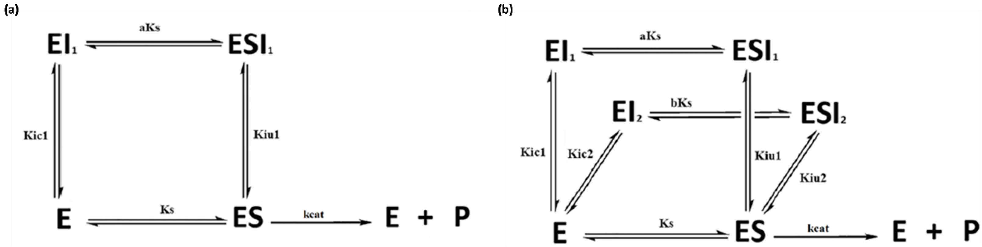
Figure 1. (a) Mixed linear inhibition model (MI), where: E—enzyme; ES—complex enzyme inhibitor; ESI—complex enzyme inhibitor substrate; EI—complex enzyme inhibitor; P—product; Km—Michaelis–Menten constant; Kic, Kiu—dissociation constants; kcat—catalytic constant. (b) Kinetic mechanism for two exclusive mixed linear inhibitors (I1 and I2) with Kiu1/Kic1 = a and Kiu2/Kic2 = b.
Applsci 12 00102 g001
Figure 2. Theoretical simulation of product versus time curves with integrated equations assuming Vmax = 18 μM min−1; S0 = 100 μM; and the following Km/Kic ratios: (a) Km/Kic = 1000; (b) Km/Kic = 5 (non-saturating conditions); (c) Km/Kic = 5 (saturating conditions); (d) Km/Kic = 0.4. The integrated equations utilized were without inhibition (solid line, Equation (1)) and in the presence of competitive inhibition by the reaction product (dashed line, Equation (2)).
Applsci 12 00102 g002
Figure 3. Scheme of theoretical framework developed in order to show that with the same data range, different kinetic models were obtained as a function of the chosen methodology (initial velocities or progress curve analysis).
Applsci 12 00102 g003
Table 1. Integrated Michaelis–Menten equations obtained from the model explained in Figure 1, assuming product inhibition [10].
Kinetic Model *Equation
WI t = 1 V m a x { K m l n [ S t ] [ S 0 ] + ( [ S t ] [ S 0 ] ) } (1)
CI t = 1 V m a x { K m ( [ S 0 ] K i c + [ I 1 ] K i c + 1 ) l n [ S t ] [ S 0 ] + ( 1 K m K i c ) ( [ S t ] [ S 0 ] ) } (2)
NCI t = 1 V m a x { K m ( [ S 0 ] K i + [ I 1 ] K i + 1 ) l n [ S t ] [ S 0 ] + ( 1 K m K i + [ I 1 ] K i + [ S 0 ] K i ) ( [ S t ] [ S 0 ] ) 1 2 K i ( [ S t ] 2 [ S 0 ] 2 ) } (3)
UCI t = 1 V m a x { K m l n [ S t ] [ S 0 ] + ( 1 + [ S 0 ] K i u + [ I 1 ] K i u ) ( [ S t ] [ S 0 ] ) 1 2 K i u ( [ S t ] 2 [ S 0 ] 2 ) } (4)
MI t = 1 V m a x { K m ( [ S 0 ] K i c + [ I 1 ] K i c + 1 ) l n [ S t ] [ S 0 ] + ( 1 K m K i c + [ S 0 ] K i u + [ I 1 ] K i u ) ( [ S t ] [ S 0 ] ) 1 2 K i u ( [ S t ] 2 [ S 0 ] 2 ) } (5)
* WI—without inhibition; CI—competitive inhibition; NCI—noncompetitive inhibition; UCI—uncompetitive inhibition; MI—mixed inhibition.
Table 2. Integrated Michaelis–Menten equations obtained from the model explained in Figure 1, considering the simultaneous presence of two mutually exclusive inhibitors when one of which is a reaction product [8].
Kinetic Model *Equation
CI t = 1 V m a x { K m ( [ S 0 ] K i c 1 + [ I 1 ] K i c 1 + [ I 2 ] K i c 2 + 1 ) l n [ S t ] [ S 0 ] + ( 1 K m K i c 1 ) ( [ S t ] [ S 0 ] ) } (6)
NCI t = 1 V m a x { K m ( [ S 0 ] K i 1 + [ I 1 ] K i 1 + [ I 2 ] K i 2 + 1 ) l n [ S t ] [ S 0 ] + ( 1 K m K i 1 + [ I 2 ] K i 2 + [ I 1 ] K i 1 + [ S 0 ] K i 1 ) ( [ S t ] [ S 0 ] ) 1 2 K i 1 ( [ S t ] 2 [ S 0 ] 2 ) } (7)
UCI t = 1 V m a x { K m l n [ S t ] [ S 0 ] + ( 1 + [ S 0 ] K i u 1 + [ I 2 ] K i u 2 + [ I 1 ] K i u 1 ) ( [ S t ] [ S 0 ] ) 1 2 K i u 1 ( [ S t ] 2 [ S 0 ] 2 ) } (8)
MI t = 1 V m a x { K m ( [ S 0 ] K i c 1 + [ I 1 ] K i c 1 + [ I 2 ] K i c 2 + 1 ) l n [ S t ] [ S 0 ] + ( 1 K m K i c 1 + [ S 0 ] K i u 1 + [ I 2 ] K i u 2 + [ I 1 ] K i u 1 ) ( [ S t ] [ S 0 ] ) 1 2 K i u 1 ( [ S t ] 2 [ S 0 ] 2 ) } (9)
* CI—competitive inhibition; NCI—noncompetitive inhibition; UCI—uncompetitive inhibition; MI—mixed inhibition.
Table 3. Sum of square error (SSE) values for different models obtained by the MME and IMME methodologies.
WICINCIUCIMI
MME
SSE0.0015990.0003400.0000330.0000100.000007
p23334
n1414141414
IMME
SSE946.511339.96219.8143.0640.0000006
p24446
n432432432432432
Table 4. Discrimination of the UCI model using AIC methodology with initial velocities data (MME).
Models A/BSSEASSEBnPA + 1PB + 1AICAAICBAICcAAICcBΔProbability
B Correct
WI/UCI0.0015990.0000101434−121.1−190.2−118.7−185.7−67.01.00
UCI/MI0.0000100.0000071445−190.2−192.4−185.7−184.90.80.397
Table 5. Summary of obtained constants with discriminated best fit models.
Method (Model)Km (μM)Kic1 (μM)Kiu1 (μM)Kic2 (μM)Kiu2 (μM)Vmax (μmol min−1 mg−1)
MME (UCI)344.4 (±17.3) -7.3 (±0.3)0.077 (±0.001)
IMME (MI)499.99 (±0.001)99.98 (±0.001)50.0 (±0.000)50.0 (±0.000)5.0 (±0.000)0.121 (±0.000)
Publisher’s Note: MDPI stays neutral with regard to jurisdictional claims in published maps and institutional affiliations.

