Abstract
Neuromorphic models are proving capable of performing complex machine learning tasks, overcoming the structural limitations imposed by software algorithms and electronic architectures. Recently, both supervised and unsupervised learnings were obtained in photonic neurons by means of spatial-soliton-waveguide X-junctions. This paper investigates the behavior of networks based on these solitonic neurons, which are capable of performing complex tasks such as bit-to-bit information memorization and recognition. By exploiting photorefractive nonlinearity as if it were a biological neuroplasticity, the network modifies and adapts to the incoming signals, memorizing and recognizing them (photorefractive plasticity). The information processing and storage result in a plastic modification of the network interconnections. Theoretical description and numerical simulation of solitonic networks are reported and applied to the processing of 4-bit information.
1. Introduction
During the twentieth century, experiments on biological neural systems led to an ever deeper understanding of some typical mechanisms of neural tissue such as learning and memory [1,2]. Physical and mathematical models have been developed to simulate the communication among basic neural units [2,3]. These models provided the basis for the development of Artificial Intelligence which, in the middle of the same century, found rapid development as software algorithms through Machine Learning (ML) and Deep Learning (DL) techniques [4]. The results were surprising: the use of AI models has revolutionized the world of data analysis and big data [5]. Neural networks are able to understand; learn; and, later on, recognize, predict, and classify. However, the AI software differences from biological analogues led the research to turn towards the realization of neural hardware systems. In a short time, the neuromorphic approach became predominant [6]. Basically, it consists in the attempt to replicate the fundamental blocks of the biological nervous system and their way of communicating. The main advantage of the neuromorphic approach lies in the possibility of having a structure capable of processing data and simultaneously retaining its memory, overcoming the dichotomy between processing and memory units imposed by the Von Neumann architecture. The electronic neuromorphic hardware has encountered physical limits mainly due to a strong energy dissipation and a poor adaptability of the structure. Moreover, neuromorphic electronics has shown memory structures based on absorption processes, which consequently increase the energy consumption necessary for network management. In this context, neuromorphic optics has been developed, bringing with it numerous advantages such as high computation speed and low losses. Photonic systems have shown fundamental properties for the management of data processing and their storage [7]. A possible approach consists in reproducing the typical functional behavior of the biological neuron. Indeed, a biological neural network is a complex structure, based on simpler units (neurons), which receives inputs, processes them, and finally produces a weighted output. The advancement of information in the network and its release is a threshold process: the incoming signals are summed and processed with respect to a reference threshold, above which the information is transmitted; otherwise, it is “forgotten” since it is classified as not “sufficiently important”. The neuronal activation threshold follows a nonlinear trend described by a sigmoid-type function. In literature, neuronal activation has been reported in plasmonic structures [8] and in hybrid plasmonic–soliton structures [9]. Deep Learning software [10] as well as electronic and optical neuromorphic hardware [11] are able to replicate this spiking operation, but usually do not retain memory. Consequently, the processing unit results separated from the memory one, unlike what happens in biological neurons, where information produces a strengthening or weakening of the synapses, i.e., the interconnections between neurons. Therefore, during learning, the network modifies by adapting to the information received through variations in the number and intensity of synaptic interconnections. The ability of solitons to create reconfigurable light channels was indeed already demonstrated [12,13,14,15,16].
More important information is recognized as stronger signals, while less important information as weaker signals. The intensity of the input signal is associated with the synaptic intensity, which characterizes the strength of the connection between two or more neurons, acting as a bridge. The synaptic activity, as a function of the intensity of the received inputs, is regulated by the variation in the density of neurotransmitters [17]. Their concentration influences the signal transmission and the synaptic formation too. When new information arrives, it is possible that new neuronal bridges are built. This phenomenon is a direct consequence of the specific migration of neurotransmitters. Biological synaptic connections are also strengthened by another factor: repetition. The reiteration of signal propagation along “neural bridges” strengthens their weight, making them privileged over others. This is a strategy widely used in the biological world called stigmergy [18,19]. The stigmergic strategy is, in general, a method of communication that uses de-centralized and spatially distributed systems, in which individuals can communicate with each other by changing their surroundings; it allows the neuronal units to increase communication by changing the structure of the synaptic connections and, therefore, of the neurons themselves.
The physical nature of the optical neural network model we present here works in a very similar way [19,20]. Such neurophotonic hardware is able to readjust its own structure according to the inputs it receives, keeping the processing information in the new conformation assumed through a plastic memory. Already, a single neuron is able both to perform both supervised and unsupervised signal recognition tasks and to memorize the signal processing by changing its structure.
In this paper, we extend the study from a single solitonic neuron to a complex network implemented by interfacing several solitonic neurons together. The extension from a single neuron to a network allows you to process larger signals in terms of number of bits. For example, a network of 5 neurons (i.e., 5 × soliton junctions), organized on 3 successive levels, is able to store 4-bit numbers and subsequently reuse this information to recognize further unknown numbers sent.
This work demonstrates that a nonlinear optical system is capable of highly effective simulation of synaptic plasticity, reinforcing interconnections and pathways in the network as a memory of stored information.
2. Biological vs. Solitonic Neural Networks
As mentioned above, here, we implement a Soliton Neural Network (SNN) interconnecting several solitonic units together. The transmission of incoming signals to the network depends on the “strength” with which the channels that make up the synaptic connections have been written. The simplest neural unit [18] is built with an X-Junction structure in which two channels, created by the propagation of photorefractive solitons, intersect at the center of the neural geometry. Among all spatial solitons and their associated waveguides, the photorefractive ones are particularly interesting for application, being generated by low-power light beams, as intense as microwatts or even nanowatts [20,21,22]. For neural purposes, we use optical signals that, propagating within soliton waveguides, can modify them by means of a local variation of the refractive index—where the refractive contrast is greater, the light will remain more confined, reinforcing that specific synaptic trajectory within the neural graph. In fact, the information will deviate towards one of the two channels of each junction as a function of the induced refractive index variation, which depends on the photogenerated electric charges. In photorefractive SNN, the photogenerated electric charges assume the functional role that the neurotransmitters play in the Biological Neural Networks (BNN): regulator of synaptic intensity. The synapse also plays another fundamental role: memory. As a connection strengthens, the neural system begins to learn an input sequence. The repetition of information results in a synaptic strengthening, which is synonymous with information memorization. Therefore, structural change (synaptic strengthening or weakening) means a memorization or an obliviation. The SNN indeed strengthens or weakens its channels according to the information (input signals) it is learning.
In summary, BNNs and SNNs learn by changing their structure according to the incoming information; a neural path is strengthened mainly based on two factors:
- Intensity of input signals;
- Persistence of signals along a specific path.
Then, the information processing is stored in the self-modification process of the structure. Figure 1 shows a summary diagram of the functionality of the two neural models, biological and solitonic, highlighting the analogous logical–structural flow that leads from input to learning and its memorization.
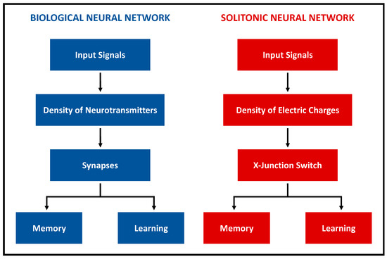
Figure 1.
Diagram of the functional parallelism between BNNs and SNNs. Both systems are able to modify their structure, to process the incoming information and to store them. The structural variations are due, in the biological case, to variations in the density of neurotransmitters, while in the solitonic case in the density of electrical charges.
3. Architecture of a Learning SNN
An SNN is formed by a set of elementary units consisting of X-junctions of soliton channels (Figure 2A). The channels are written by soliton beams of equal light power in order to create balanced 50−50 junctions. In order to limit the luminous powers used, photorefractive crystals are used as substrates, which allow the soliton formation already at powers of tens of nanowatts.
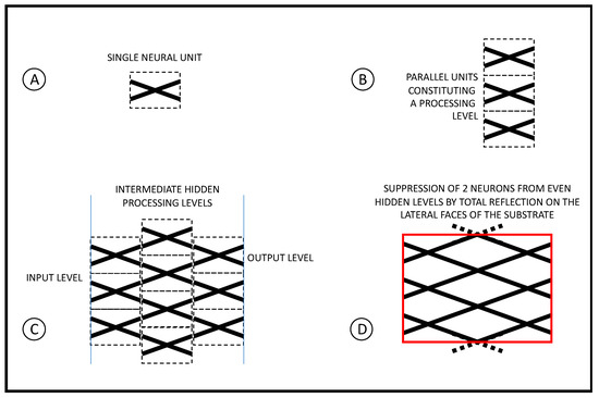
Figure 2.
Schematic architecture of an SNN used for bit-to-bit storage of information. (A) A single neural unit structure is constituted by a single X-junction; (B) one processing level in the network consists of several units in parallel; (C) successive levels of the network are connected in series with each other; (D) even-order levels have two fewer units. The suppression of these units is replaced with the insertion of the total reflections at the lateral edges of the substrate.
As in normal neural networks, even the solitonic ones are divided into successive levels, each formed by elementary units connected in parallel (Figure 2B,C).
The first input level is identified with the input face: it is formed by a number of elementary units identified by the number of bits of the information to be processed. Since each elementary unit has N inputs, the number of units used in the input layer is N/2. Similarly, the output level consists of the output face: for episodic memory applications, the number of output channels must coincide with the number of bits to be processed.
Between the input and the output, hidden computational levels are inserted, which switch their junctions according to the information sent and must be memorized. Odd hidden levels contain N/2 elementary units while even hidden levels contain N/2-2 elementary units: the suppression of these 2 units is substituted by a total reflection from the substrate boundary. The number of hidden levels is chosen in order to ensure the complete overlap of all the information with the others: in this way, the network is able to keep a unique memory of the information sent.
4. Mathematical Model of the SNN
The elementary unit of an SNN has already demonstrated its ability to perform both supervised [18] and unsupervised [19] learning. In both cases, the X-junction contained in the elementary unit changes, switching its state from the initial neutral condition 50−50 to the final unbalanced one 80−20. This dynamic corresponds to the learning process of the single unit, and it is mathematically described by the matrix expression:
where X and Y are the input and output vectors, respectively, and W is the gate transfer matrix, which depends on the photorefractive bias EBias on the input values xi. W is not constant and can change according to the learning of the unit. As can be observed, the matrix is nonlinear, which means it depends on X values as well. Therefore, the resolution of Equation (1) occurs recursively, as the learning process is “slow”—that is, it requires reinforcing over time the information channel to be stored.
The general expression of W is given by
where
describes the normalized balance of the i-th channel at the previous iteration time, and
the normalized signal injected in the i-th channel at the time t. In both Equations (3) and (4), describes the power of the dark radiation circulating within the network.
The parameter χ in Equation (2) refers to the energy that has previously flowed through the junction with respect to the maximum possible saturation level, thanks to the SAT parameter. This defines the saturation dynamics and the structure imbalance values
The SAT parameter is the one responsible for the unbalance dynamics of each single unit. Different SAT values lead to different unbalance values (called here, SJR: Single Junction Ratio) of the elementary units of the SNN, as shown in Table 1.

Table 1.
Unbalance obtained between the two channels of the soliton neuron after 20 iterations of the mathematical model as a function of the SAT parameter.
Starting from the transfer matrix of a single elementary unit in Equation (1), the model is extended to the whole network, analyzing the input–output interconnections between units. The input level, as described above, defines the input signals; therefore, it is not a processing but a definition level (Figure 2C). Then, the model analyses the interconnections between elementary units in the hidden levels: the outputs of the previous level constitute the inputs of the next one and so on.
5. A 4-Bit SNN Working as an Episodic Memory
An Episodic Memory is a system that is able to store the received information bit-to-bit (training phase), recall, and use them to recognize further unknown information (testing phase). Such a kind of memory stores them as they are: in fact, it is very similar (at least for the training phase) to traditional electronic memories, which store strings of bytes that can be recalled later. We have applied the SNN theory to realize a 4-bit episodic memory network, built using two elementary units in parallel organized into 3 hidden levels, as shown in Figure 3.
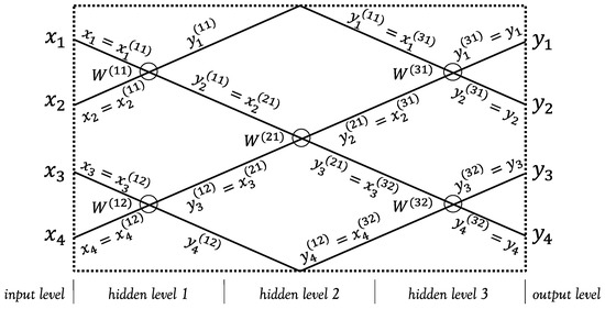
Figure 3.
Structural scheme of the SNN used as an episodic memory. W represents the computational weight of the node. W(1) is the computational weight relative to the node of the first neuron in Layer 1; W(2) is the computational weight relative to the node of the second neuron in Layer 2; W(3) is the computational weight relative to the node of the neuron in Layer 2; W(4) is the computational weight relative to the node of the first neuron in Layer 3; W(5) is the computational weight relative to the node of the first neuron in Layer 3. The inputs at the entrance to the network are xi while the signals at the end of the whole processing are yi.
The adopted notation numbers the signals from 1 to 4 going from top to bottom at every level, as shown in the diagram of Figure 3. The number of hidden levels was chosen to let all signals recombine with each other: this condition is essential to ensure the storage of the entire 4-bit signal. Being a 4-bit network, in the input level and in the first hidden level there are 2 elementary units in parallel (computing neurons) that carry out a first processing of the information; the results of the first hidden level are carried over to the second. Being an even level, it contains only one elementary unit, which analyzes signals 2−3, while signals 1−4 are transferred to the third level as they are. The third level processes the latest information: its outputs constitute the outputs of the entire network.
Then, the whole network learns through a subsequent reprocessing of the signals, which are transferred from the input to the output through successive iterations. Therefore, the single calculation units switch on the basis of the received signals, consequently varying the weights of each node. We can now consider a matrix transfer relationship for the whole network similar to Equation (1) written for the single elementary unit, where the inputs and outputs are now vectors of dimension 4, which contain the 4 bits to be analyzed.
Each layer will have its own weight transfer matrix, composed of the matrices of the single units used by the number of signal processing nodes. The odd layers of the network, layers 1 and 3, both have very similar transfer matrices as they both contain 2 elementary units in parallel. The form of such matrices is Wj=1,3 is
where j-odd = 1,3 indicates the layer number, and
The matrix transfer function for the even Wj=2 is instead
At each iteration, the network nodes are affected by the passage of the writing signals, which determine the switch towards one output or the other.
As shown in Table 1, the SAT parameter determines the single unit unbalancement. Thus, we have analyzed the learning of the 4-bit network for the three possible umbalancing cases of the single unit (i.e., 0.7−0.3, 0.8−0.2, 0.9−0.1) by varying the input information number.
Table 2 shows output signals in the case of single launched signal at a time.
Table 2.
Results of the simulation outputs of the mathematical model for 1-digit, 4-bit numbers and for different SJR values: (a) SJR = 0.7−0.3, (b) SJR = 0.8−0.2, and (c) SJR = 0.9−0.1.
As it can be seen from the table, for all input numbers there is an output channel showing a higher intensity than the others, as expected. However, the contrast of the output channels increases with the switching efficiency of each single junction: for SJR = 0.7−0.3, the contrast of the output channel is limited in the range 1.3–9.0, arriving up to 8–103 for SJR = 0.9−0.1.
Figure 4 shows the SNN learning map evolution along the three layers for the three cases reported in Table 1. It is interesting to note that, in all cases, the signals flow towards the outputs opposite to their corresponding input channels, as expected from a solitonic behavior [18,19]. We shall see this phenomenon in the following paragraph. For higher SAT values (i.e., higher SJR), this redistribution is faster (Figure 4c). From a graphic point of view, the strength of learning, corresponding to the ability to more unbalance each node of the network towards one output rather than the other, is represented through a sharper contrast between the colors. This dynamic is visible in Figure 4, Figure 5 and Figure 6 (for numbers consisting of more than 1 digit) through the signal flow directions, which consequently represent the learning dynamics of the entire neuronal network.
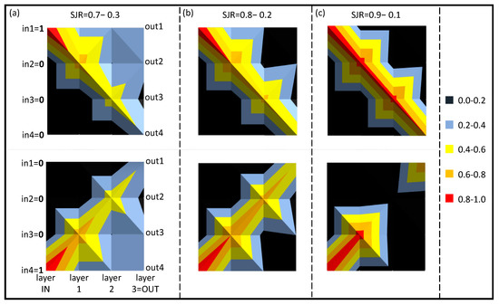
Figure 4.
Represents the evolution of the intensities in the three layers with respect to the two input configurations, 1−0−0−0 and 0−0−0−1 (1-digit, 4-bit numbers), for the three cases of SJR: (a) SJR = 0.7−0.3; (b) SJR = 0.8−0.2; (c) SJR = 0.9−0.1.
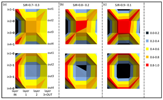
Figure 5.
Represents the energy flow in a three-layer network learning two input numbers, 1−0−0−1 and 0−1−1−0, for the three SJRs: (a) SJR = 0.7−0.3; (b) SJR = 0.8−0.2; (c) SJR = 0.9−0.1.
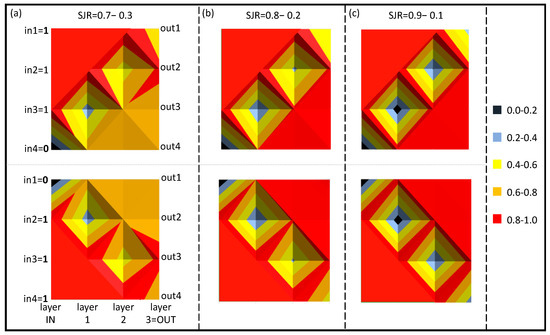
Figure 6.
Represents the evolution of the intensities in the three layers with respect to the three input configurations, 1−1−1−0 and 0−1−1−1, for the three cases of imbalance: (a) SJR = 0.7−0.3; (b) SJR = 0.8−0.2; (c) SJR = 0.9−0.1.
The SNN learning map evolution has been investigated also in the case of 4-bit numbers constituted by two ones and two zeros (2-digit, 4-bit numbers). Table 3 reports the output patterns for each input permutation, while Figure 5 represents the signals’ flow in all channels.
Table 3.
Results of the simulation outputs of the mathematical model for 2-digit, 4-bit numbers and for different SJR values: (a) SJR = 0.7−0.3, (b) SJR = 0.8−0.2, and (c) SJR = 0.9−0.1.
Each evolution, connected to a precise input pattern, is characterized by a specific signal pattern that becomes more and contrasted as the SJR values increase. This is indeed expected and will be also more evident with the solitonic simulations.
Finally, the 4-bit SNN is capable of efficiently recognizing and storing patterns triggered by three input signals as well (3-digit, 4-bit numbers). Table 4 reports the learning configurations for this case and increasing SJR values. As can be seen, all outputs show 3 channels with high values and one with a low one. The contrast follows the SJR value.
Table 4.
Results of the simulation outputs of the mathematical model for 3-digit, 4-bit numbers and for different SJR values: (a) SJR = 0.7−0.3, (b) SJR = 0.8−0.2, and (c) SJR = 0.9−0.1.
The evolution of signals in the network follows specific patterns (Figure 6), whose contrast increases as the SJR parameter increases too.
6. Comparison with the SNN Dynamics
The generation of the photorefractive soliton network was schematized following the experimental configuration used for a single X-junction [18]. We considered a lithium niobate crystal as large as 150 μm along the x and y axes and 10 mm along the propagation axis (z axis). The experimental numerical parameters used in the simulations are reported in Table 5. Four equal intensity write beams were injected into the input to create the initial balanced network.
Table 5.
Numerical parameters used in the soliton simulations.
These beams cross in pairs and then totally reflect at the substrate boundaries [23,24,25] to recreate the geometry of the network previously described in Figure 3. The result is a perfectly balanced network, which means that if any further signal propagating inside a waveguide reaches the crossing, it will be split 50-50 to the output channels. Thus, it represents a virgin network from the point of view of learning.
Each elementary unit (neuron) is formed by a X-junction [14], whose small angle of about 1° allows for coupling between the crossing channels. The learning dynamics of the network derive from the imbalance of each single junction (SJR), following a logic of distributed intelligence.
The complex 4-bit SNN network used here follows the functional scheme described above, using a cascade protocol for which the inputs of a deeper level of the network correspond to the outputs processed by the previous one.
The behavior of the 4-bit soliton network was simulated using a well-tested FDTD numerical code [26], which solves the nonlinear wave equations in Slowly Varying Envelope Approximation. Figure 7 shows the flow chart of the solver.
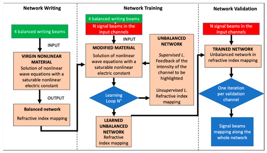
Figure 7.
The solver code is divided into three sections: the first one writes a balanced network based on X-junction units by solving the nonlinear wave equations of four light beams within a nonlinear medium. The output of this section corresponds to the refractive index mapping of the junction, which is now used as the initial structure for the propagation of N signal beams, which are injected into 4 input arms (i.e., an N-digit, 4-bit number). The signal beams would slightly modify specific channels of the network arms. By recursive feedbacks, the network slowly learns the inserted information. The last phase is then the testing one: using a single iteration, further “unknown” signals enter the trained refractive index mapping and generate specific output patterns, depending on whether they are recognized or not.
The numerical code is divided into three consecutive sessions. The first one is used to write the network structure, the second one for the training process, and the third one for the testing process. In the first phase, Network Writing, four visible light beams, with transverse hyperbolic secant profiles, are injected inside a virgin medium with saturating electro-optical nonlinearity:
where is the linear extraordinary refractive index, with Ee representing the electric field present along the extraordinary direction of the crystal, which is the sum of the bias and the locally induced screening.
These beams experience self-confinement, propagating without diffraction similar to spatial solitons. The particular geometry ensures that the beams intersect with each other according to the scheme described in Figure 3. In this way, the neural network is created in the initial configuration—that is, with all the intersections (i.e., the elementary neurons) perfectly balanced.
In the second phase, Network Training, the network is modified according to the information signals injected into the input channels. Signal beams are at a wavelength longer than the writing ones but still absorbed: as a consequence, signal beams are able to excite charges and to induce nonlinearity too, with lower efficiency due to the longer wavelength. Their propagation inside the soliton channels is indeed nonlinear in nature, reinforcing the nonlinear refractive index constrast of the used channel by means of an increasing of the local screening electric field. Through successive iterations, the nonlinearity excited by the signals writes deeper soliton channels (higher contrast of the refractive index), consequently also unbalancing all the junctions of the network. In this way, the whole integrated system learns the information sent, writing specific trajectories in the network of solitonic waveguides (data storage as propagation patterns). The training phase coincides with the learning operation. To test the learning efficiency, in the Network Validation phase, all 4-bit numbers are sent to the input; among all the possibilities, only the one corresponding to the number stored through the specific propagation pattern in the network will be recognized. Different numbers with respect to writing will lead the signals to propagate along trajectories that have not been highlighted and, consequently, their output will be low (number not recognized).
6.1. Learning and Memorization Processes
In the Network Writing phase, the numerical code creates the perfectly balanced network shown in Figure 8. In this case, the network is made up of perfectly balanced junctions and is ready to receive the information to be memorized.
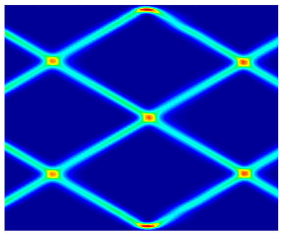
Figure 8.
Perfectly balanced SNN network. At this stage, the network is ready to accept input information and change according to them.
To test the plastic learning capabilities of the network, three data configurations were created and used:
- ▪
- Single input beam, which corresponds to a single illuminated pixel in a 4 × 4 pixel matrix (1-digit, 4-bit numbers);
- ▪
- Two input beams, which correspond to two illuminated pixels (2-digit, 4-bit numbers);
- ▪
- Three input beams, which correspond to three illuminated pixels (3-digit, 4-bit numbers).
6.1.1. 1-Digit, 4-Bit Numbers
Four different training runs were carried out, one for each number to be memorized, as shown in the first raw of Figure 9. In the validation phase, for each memorization, all four numbers were sent and the network response was analyzed. A stronger response is expected when the validation number and the stored one coincide. In this case, the system response is expected to exceed a threshold, which is set as a percentage of the input signal value:
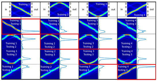
Figure 9.
Training and testing phases are reported for 1-digit, 4-bit numbers. In the first raw, the training phases are reported. In the following raws, the testing experiments are reported. Those for which training and testing numbers coincide are framed in red.
From simulations, θ is about ~0.7 (measured value).
When validation and stored numbers do not coincide, a low output response is expected, which means nonrecognition. Figure 9 summarizes all the possibilities for 1-digit, 4-bit numbers, both in terms of training/memorization and validation.
The first line shows the network training with the four 1-digit value 1 and 4-digit value 0. The images below show the use of the stored information to recognize any new numbers sent. If digit 1 of the new number corresponds to digit 1 of the training number, the output is high, otherwise the signal remains low, below threshold. The figure shows all 16 possible test cases for the 4 trainings carried out. The red frames in the figure highlight the tests carried out for the same training and test numbers. In all these cases, the output signal is much greater than when the test is performed with non-coincident numbers.
Figure 10 shows how the amplitudes of the output signals vary as a function of the training channel. The dashed line represents the threshold value for passing validation.
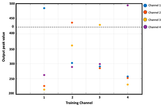
Figure 10.
Amplitudes of the output signals for the different training numbers. As shown, for each training number, there is only one channel whose amplitude exceeds a threshold value identified by the dashed horizontal line.
From the figure, channels 1 and 4 show higher outputs than channels 2 and 3; therefore, they are less subject to attenuation: this is probably related to the geometry of the device, which leads them to have no reflections on the edges, unlike what happens for channels 2 and 3.
6.1.2. 2-Digit, 4-Bit Numbers
We trained and then tested the soliton neural network with all six 2-digit, 4-bit numbers as well (Figure 11). Again, we expect high outputs in validation when training and test numbers coincide. However, high test output signals are also found when not both trained channels are used but only one, which corresponds to a partial recognition of the information.
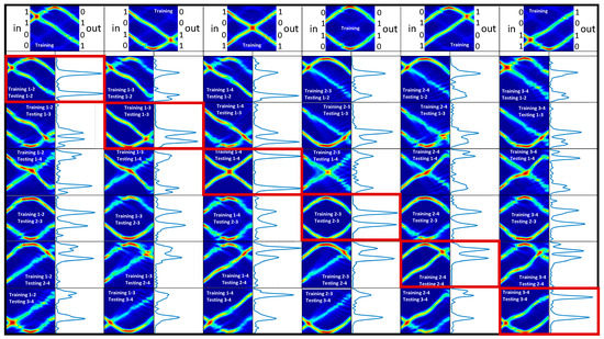
Figure 11.
Training and testing phases are reported for 2−digit, 4−bit numbers. In the first raw, the training phases are reported. In the following raws, the testing experiments are reported. Those for which training and testing numbers coincide are framed in red.
Figure 12 shows the channel output values for all test cases performed. As shown, for each training number, there is only one number where both outputs exceed the threshold (dashed line). In the other cases, if one of the inputs coincides with a trained channel, the output will be high; otherwise, it will be low.
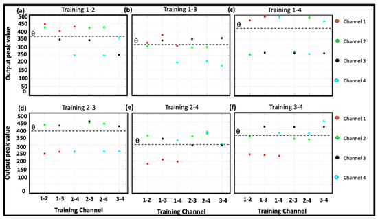
Figure 12.
Amplitudes of the output signals for the different training 2-digit, 4-bit numbers. As shown, for each training number, there is only one case in which both outputs exceed the threshold (dashed horizontal line): (a–f) report the cases of validation after having trained the possible combinations of channels respectively. However, the network is also able to recognize single-trained digits.
Therefore, the network is able both to recognize the complete number and only some of the digits used. Clearly, the outputs of complete numbers have higher values than those in which a single digit is recognized.
6.1.3. 3-Digit, 4-Bit Numbers
The SNN network learning behavior has been studied also for the recognition of three illuminated pixels. The training procedure follows the scheme of the two cases previously described.
Figure 13 shows the training and testing phases for each possible combination of numbers with three activated pixels. The results of the amplitudes of the test signals are shown in Figure 14. In this case, as in the previous case of 2-digit numbers, for each training there is only one recognized number with 3 suprathreshold outputs. As in the previous case, the network is also able to recognize individual trained channels.
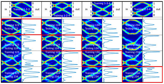
Figure 13.
Training and testing phases are reported for 3-digit, 4-bit numbers. In the first raw, the training phases are reported. In the following raws, the testing experiments are reported. Those for which training and testing numbers coincide are framed in red.
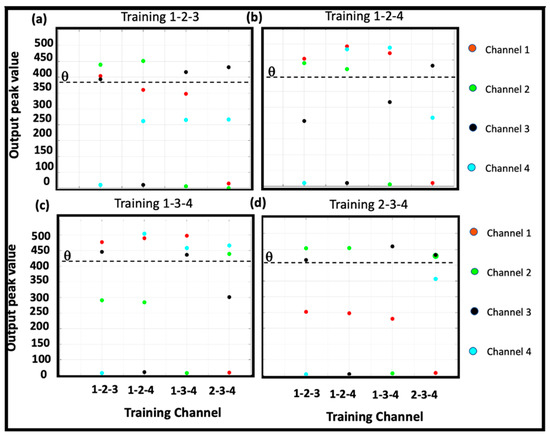
Figure 14.
Amplitudes of the output signals for the different training 2-digit, 4-bit numbers. As shown, for each training number, there is only one case in which both outputs exceed the threshold (dashed horizontal line): (a–d) report the cases of validation after having trained the possible combinations of channels respectively. However, the network is able to recognize also single trained digits.
6.2. Materials and Memorization
Photorefractive materials have very different characteristics: there are materials with very fast responses (InP, BSO etc…), medium responses (SBN), and very slow responses (LiNbO3). Often, these materials show an intrinsic memory, in the sense that the photoexcited charges can be localized in states that can hardly relax. For example, bulk crystals of lithium niobate showed extremely slow dielectric relaxations, considered almost permanent: soliton waveguides in these crystals might be still active months after their writing [22].
Materials with different dielectric relaxation rates can be used for different purposes: very fast response systems can create RAM memory networks while slow response materials can constitute semipermanent or fully permanent ROM storage structures.
However, recently, it has been experimentally observed that reducing the size of the nonlinear crystals down to a few microns in thickness determines an acceleration of the nonlinear response of many orders of magnitude [27,28]. By using thin films, it is possible to obtain photorefractive responses even at the nanosecond. Furthermore, it has been observed that the reduced total size of the crystal favors the charge movement, allowing rapid photorefractive relaxations up to the complete optical erasing of the excited structures [29].
7. Conclusions
The study carried out effectively demonstrates that an SNN is able to reproduce the functionality of an episodic memory, learning numbers as sequences of bits through modifications of the network itself. The neuroplasticity of the photorefractive refractive index allows the network to modify itself, learning specific propagation trajectories that act as a memory of the information that wrote it. By doing so, the network is also able to recognize unknown information that is sent to it, as only that which is sent in channels they have learned will come out vigorous in the end. The network thus stores and processes in the same physical position, eliminating the dichotomy typical of traditional processing systems based on Von Neumann’s circuit geometries, and following the neuromorphic paradigm (i.e., the coincidence of memory and calculation areas). The functional characteristics of an SNN reproduce the dynamics of biological neural networks: learning and memorization occur through a physical modification of the structure. This plasticity is due to several mechanisms whose dynamics are similar. In the biological nervous system, the density shift of neurotransmitters is responsible for the creation and modification of synapses, while in soliton neural networks, the construction of X-junctions depends on the density of the photoexcited electrical charges.
Author Contributions
Conceptualization, A.B. and E.F.; methodology, A.B., H.T. and E.F.; investigation, A.B.; writing—review and editing, A.B. and E.F.; supervision, E.F.; project administration, E.F. All authors have read and agreed to the published version of the manuscript.
Funding
Open access funding provided by Sapienza Università di Roma within the CRUI-CARE Agreement. Sapienza Università di Roma—Avvio alla Ricerca (AR12117A814F8BCA). Sapienza Università di Roma—bando SEED-PNR contract 000300_21_RS_FAZIO_SEED_PNR_2021. AMDG.
Institutional Review Board Statement
Not applicable.
Informed Consent Statement
Not applicable.
Data Availability Statement
Not applicable.
Conflicts of Interest
The authors declare no conflict of interest.
References
- Kandel, E.R. Search of Memory; Editions Code; 2017; ISBN 978-88-7578-675-5. [Google Scholar]
- Gerstner, W.; Kistler, W.M.; Naud, R.; Paninski, L. Neuronal Dynamics: From Single Neurons to Networks and Models of Cognition; Cambridge University Press: Cambridge, UK, 2014. [Google Scholar]
- Denz, C. Optical Neural Networks; Tschudi, T., Ed.; Springer International Publisher: Wiesbaden, Germany, 1998. [Google Scholar] [CrossRef]
- Goodfellow, I.J.; Bengio, Y.; Courville, A. Deep learning. Genet. Program. Evolvable Mach. 2018, 19, 305–307. [Google Scholar] [CrossRef]
- Bile, A.; Tari, H.; Grinde, A.; Frasca, F.; Siani, A.M.; Fazio, E. Novel Model Based on Artificial Neural Networks to Predict Short-Term Temperature Evolution in Museum Environment. Sensors 2022, 22, 615. [Google Scholar] [CrossRef]
- Schuman, C.D.; Potok, T.E.; Patton, R.M.; Birdwell, J.D.; Dean, M.E.; Rose, G.S.; Plank, J.S. A Survey of Neuromorphic Computing and Neural Networks in Hardware. arXiv 2017, arXiv:1705.06963. [Google Scholar]
- Bile, A.; Pepino, R.; Fazio, E. Study of magnetic switch for surface plasmon-polariton circuits. AIP Adv. 2021, 11, 045222. [Google Scholar] [CrossRef]
- Tari, H.; Bile, A.; Moratti, F.; Fazio, E. Sigmoid Type Neuromorphic Activation Function Based on Saturable Absorption Behavior of Graphene/PMMA Composite for Intensity Modulation of Surface Plasmon Polariton Signals. Plasmonics 2022, 1–8. [Google Scholar] [CrossRef]
- Hesamian, M.H.; Jia, W.; He, X.; Kennedy, P. Deep Learning Techniques for Medical Image Segmentation: Achievements and Challenges. J. Digit. Imaging 2019, 32, 582–596. [Google Scholar] [CrossRef]
- Lugnan, A.; Katumba, A.; Laporte, F.; Freiberger, M.; Sackesyn, S.; Ma, C.; Gooskens, E.; Dambre, J.; Bienstman, P. Photonic neuromorphic information processing and reservoir computing. APL Photon. 2020, 5, 020901. [Google Scholar] [CrossRef]
- Scimemi, A.; Beato, M. Determining the Neurotransmitter Concentration Profile at Active Synapses. Mol. Neurobiol. 2009, 40, 289–306. [Google Scholar] [CrossRef]
- Yoshimura, T.; Roman, J.; Takahashi, Y.; Wang, W.C.V.; Inao, M.; Ishitsuka, T.; Tsukamoto, K.; Aoki, S.; Motoyoshi, K.; Sotoyam, W. Self-Organizing Lightwave Network (SOLNET) and Its Application to Film Optical Circuit Substrates. IEEE Trans. Com. Pack. Tech. 2001, 24, 500–510. [Google Scholar] [CrossRef]
- Yoshimura, T.; Inoguchi, T.; Yamamoto, T.; Moriya, S.; Teramoto, Y.; Arai, Y.; Namiki, T.; Asama, K. Self-Organized Lightwave Network Based on Waveguide Films for Three-Dimensional Optical Wiring Within Boxes. J. Lightwave Tech. 2004, 22, 2091–2101. [Google Scholar] [CrossRef]
- Xu, Z.; Kartashov, Y.V.; Torner, L. Reconfigurable soliton networks optically-induced by arrays of nondiffracting Bessel beams. Opt. Express 2005, 13, 1774–1779. [Google Scholar] [CrossRef] [PubMed]
- Xu, Z.; Kartashov, Y.V.; Torner, L.; Vysloukh, V.A. Reconfigurable directional couplers and junctions optically induced by nondiffracting Bessel beams. Opt. Lett. 2005, 30, 1180–1182. [Google Scholar] [CrossRef] [PubMed][Green Version]
- Yoshimura, T.; Nawata, H. Micro/nanoscale self-aligned optical couplings of the self-organized lightwave network (SOLNET) formed by excitation lights from outside. Opt. Comm. 2017, 383, 119–131. [Google Scholar] [CrossRef]
- Biagio, I.; Bile, A.; Alonzo, M.; Fazio, E. Stigmergic Electronic Gates and Networks. J. Comput. Electron. 2021, 20, 2614–2621. [Google Scholar]
- Alonzo, M.; Moscatelli, D.; Bastiani, L.; Belardini, A.; Soci, C.; Fazio, E. All-Optical Reinforcement Learning In Solitonic X-Junctions. Scie. Rep. 2018, 8, 5716. [Google Scholar] [CrossRef] [PubMed]
- Bile, A.; Moratti, F.; Tari, H.; Fazio, E. Supervised and Unsupervised learning using a fully-plastic all-optical unit of artificial intelligence based on solitonic waveguides. Neural Comput. Appl. 2021, 33, 17071–17079. [Google Scholar] [CrossRef]
- Wise, F.W. Solitons divide and conquer. Nature 2018, 554, 179–180. [Google Scholar] [CrossRef]
- Hendrickson, S.M.; Foster, A.C.; Camacho, R.M.; Clader, B.D. Integrated nonlinear photonics: Emerging applications and ongoing challenges—A mini review. J. Opt. Soc. Am. B Opt. Phys. 2021, 31, 3193–3203. [Google Scholar] [CrossRef]
- Fazio, E.; Renzi, F.; Rinaldi, R.; Bertolotti, M.; Chauvet, M.; Ramadan, W.; Petris, A.; Vlad, V.I. Screening-photovoltaic bright solitons in lithium niobate and associated single-mode waveguides. Appl. Phys. Lett. 2004, 85, 2193–2195. [Google Scholar] [CrossRef]
- Jäger, R.; Gorza, S.P.; Cambournac, C.; Haelterman, M.; Chauvet, M. Sharp waveguide bends induced by spatial solitons. Appl. Phys. Lett. 2006, 88, 061117. [Google Scholar] [CrossRef]
- Fazio, E.; Alonzo, M.; Belardini, A. Addressable Refraction and Curved Soliton Waveguides Using Electric Interfaces. Appl. Sci. 2019, 9, 347. [Google Scholar] [CrossRef]
- Alonzo, M.; Soci, C.; Chauvet, M.; Fazio, E. Solitonic waveguide reflection at an electric interface. Opt. Expr. 2019, 27, 20273–20281. [Google Scholar] [CrossRef] [PubMed]
- Pettazzi, F.; Coda, V.; Fanjoux, G.; Chauvet, M.; Fazio, E. Dynamic of second harmonic generation in photovoltaic photorefractive quadratic medium. J. Opt. Soc. Am. B 2010, 27, 1–9. [Google Scholar] [CrossRef]
- Chauvet, M.; Bassignot, F.; Henrot, F.; Devaux, F.; Gauthier-Manuel, L.; Maillotte, H.; Ulliac, G.; Sylvain, B. Fast-beam self-trapping in LiNbO3 films by pyroelectric effect. Opt. Lett. 2015, 40, 1258–1261. [Google Scholar] [CrossRef] [PubMed]
- Bile, A.; Chauvet, M.; Tari, H.; Fazio, E. Addressable photonic neuron using solitonic X-junctions in Lithium Niobate thin films. Opt. Lett. submitted.
- Bile, A.; Chauvet, M.; Tari, H.; Fazio, E. All-optical erasing of photorefractive solitonic channels in Lithium Niobate thin films. Opt. Lett. submitted.


Publisher’s Note: MDPI stays neutral with regard to jurisdictional claims in published maps and institutional affiliations. |
© 2022 by the authors. Licensee MDPI, Basel, Switzerland. This article is an open access article distributed under the terms and conditions of the Creative Commons Attribution (CC BY) license (https://creativecommons.org/licenses/by/4.0/).