Hydrogeochemical Survey along the Northern Coastal Region of Ramanathapuram District, Tamilnadu, India

Abstract

Ramanathapuram is a drought-prone southern Indian district that was selected for conducting a hydrogeochemical study. Groundwater samples from 40 locations were collected during January 2020 (pandemic interdiction according to COVID) and January 2021. The hydrogeochemical properties of the groundwater samples were evaluated and compared with drinking water regulations to assess their water quality. The order of cation dominance was as follows: Na⁺ > Ca²⁺ > K⁺ > Mg²⁺ in January 2020 and Na⁺ > Ca²⁺ > Mg²⁺ > K⁺ in January 2021 with respect to the mean value. The order of anion dominance was as follows: Cl⁻ > HCO₃⁻ > SO₄²⁻ > NO₃⁻ > F⁻ in January 2020 and Cl⁻ > SO₄²⁻ > HCO₃⁻ > NO₃⁻ > F⁻ in January 2021 with respect to the mean value. In the study area, the southern coastal region was identified as a groundwater-polluted zone through spatial analysis based on all analysis results. The irrigation water quality was analyzed using various calculated indices, such as Na% (percent sodium), SAR (sodium absorption ratio), PI (permeability index), MgC (magnesium risk), RSC (residual sodium concentration), and KI (Kelly ratio), demonstrating the suitability of the groundwater for irrigation in most parts of the study area. This was also confirmed by the Na% vs. EC Plot, USSL, and Doneen’s Plot for PI. In addition, the WQI results for drinking water and irrigation confirmed the suitability of the groundwater in most parts of the study area, except for the coastal regions. The dominant hydrogeologic facies of Na⁺-Cl⁻, Ca²⁺-Mg²⁺-SO₄²⁻, and Ca²⁺-Mg²⁺-Cl⁻ types illustrated by the Piper diagram indicate the mixing process of freshwater with saline water in the coastal aquifers. Rock–water interaction and evaporation were the main controllers of groundwater geochemistry in the study area, as determined using the Gibbs plot. Ion exchange, seawater intrusion, weathering of carbonates, and the dissolution of calcium and gypsum minerals from the aquifer were identified as the major geogenic processes controlling groundwater chemistry using the Chadha plot, scatter plot, and Cl⁻/HCO₃⁻ ratio. Further, multivariate statistical approaches also confirmed the strong mutual relationship among the parameters, several factors controlling hydrogeochemistry, and grouping of water samples based on the parameters. Appropriate artificial recharge techniques must be used in the affected regions to stop seawater intrusion and increase freshwater recharge.

1. Introduction

All over the world, many researchers have studied the hydrogeochemistry of various coastal aquifers for quality analysis and seawater intrusion [1,2,3,4,5,6,7]. In several coastal cities, groundwater serves as one of the freshwater sources for drinking, domestic, irrigation, and industrial needs. Seawater intrusion is considered a common problem in most coastal aquifers worldwide [8,9]. Conditions such as tidal activities, backwater in estuaries and lagoons, low hydraulic gradient in coastal regions, sea level rise, lower infiltration rates, local hydrogeological conditions, and overexploitation are the reasons for saltwater intrusion into nearshore aquifers [10,11,12,13,14]. As a result, the use of many drinking water wells and numerous farms near the coast has come to a halt due to saline groundwater. Rapid industrialization and urbanization along coastal regions make it necessary to study the effects of increased anthropogenic pressure on the dynamics of hydrogeochemistry in these areas. Hydrogeochemistry needs to be studied to identify the controlling factors and gain a comprehensive understanding of the source, origin, distribution, and driving force of organic and inorganic compounds in various coastal aquifers [15,16,17].

Environmental conditions, such as the geological and hydrogeological settings in which groundwater occurs, can be studied through hydrogeochemical investigations [18,19,20,21]. The assessment of saline water intrusion into nearshore aquifers based on groundwater geochemistry has been successfully conducted by several authors [22,23,24,25,26]. The number of groundwater resources is estimated to be 30 million. They are the sole drinking water supply for most rural households in India, but they are rapidly becoming a serious problem due to overexploitation and degradation [9,27,28]. In addition to natural processes, anthropogenic contaminants of municipal wastewater, leachates from landfills, agricultural fertilizers as return flow from irrigation, and industrial effluents are other important factors in water quality degradation [29,30]. Comprehensive studies of water quality in shallow aquifers in coastal areas have shown that the existing groundwater is of poor quality and exceeds the drinking water limits set by the WHO [18,31,32].

Hydrogeochemical analysis is a valuable tool for identifying the processes responsible for groundwater chemistry [33,34]. The hydrogeochemical processes of the groundwater system help to understand the contributions of rock–soil–water interactions [22,35,36]. Geochemical processes such as oxidation and reduction reactions, carbonate equilibrium, adsorption, and desorption occur as groundwater moves through the soil medium, which plays an important role in hydrogeochemical evolution and seasonal spatial variations in groundwater geochemistry [37,38]. The ability to monitor the suitability of water for a particular use requires determining the quality of groundwater. Anthropogenic activities have the potential to alter the relative contributions of natural sources to variability, and cause introduce pollution effects [18,21,39].

Periodic groundwater analysis is a typical approach to determine seawater intrusion into aquifers in coastal areas [40,41]. There has been no scientific publication regarding groundwater quality in the present study area. In this work, a comprehensive study was conducted to evaluate the geochemical processes that regulate groundwater quality [9]. This study suggests that the analysis of groundwater quality based on various attributes can reveal the hydrogeochemical characteristics and the need for the regulation of water quality factors in this coastal region.

The objective of the present research work is to understand the geochemistry of groundwater in a part of the Ramanathapuram district in Tamil Nadu, India. The main objectives are (i) to study the physico-chemical parameters and spatial variations of cations and anions, (ii) to determine the drinking and irrigation quality of groundwater, (iii) to identify the geogenic processes that degrade groundwater, and (iv) to study the intrusion of seawater into the coastal aquifer.

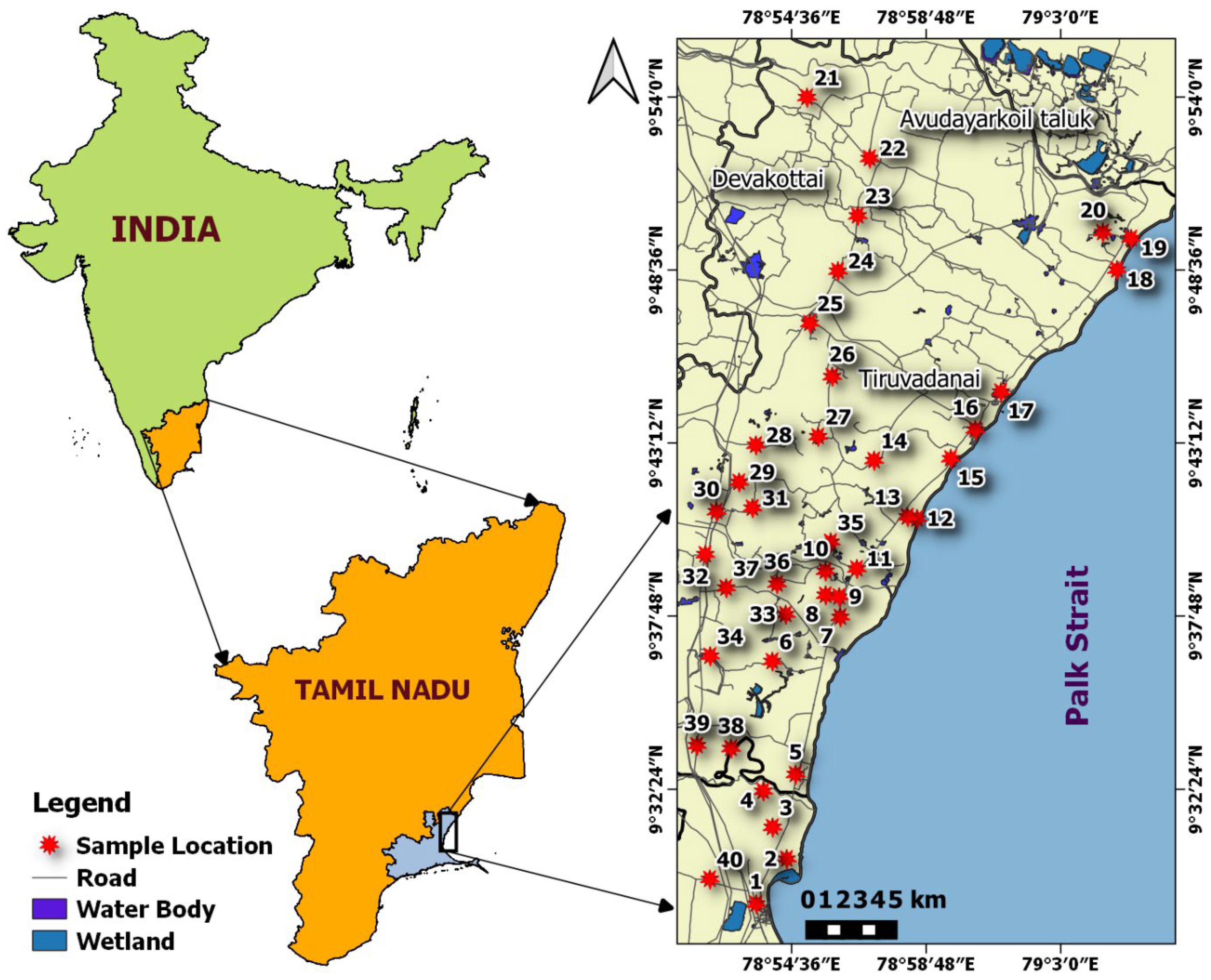
2. Study Site Description

The selected study site is part of the northern coastal zone of Ramanathapuram district, as shown in Figure 1, and covers an area of 739 km² with a 52 km-long coastline. The Ramanathapuram district is surrounded by the districts of Pudukkottai to the north, Sivagangai to the northwest, Virudhunagar and Tuticorin to the west, the Gulf of Manner to the south, and the Bay of Bengal and the Palk Strait to the east. A coastal strip projects as Rameswaram Island, which is separated from the mainland by the Palk Strait. The district’s headquarters are located in Ramanathapuram. It lies between 9°05′ N and 10°0′ N latitude and 78°10′ E and 79°30′ E longitude, with the study area lying between 9°30′–9°58′ latitude and 78°50′–78°10′ longitude. The topography of the district is generally flat terrain. The main rivers in the district are the Vaigai and the Gundar. During the summer season, these rivers are usually dry. The district covers a geographical area of 4207.38 km². The prevailing tropical climate is typical for this region. The district is characterized by a high level of aridity. A cool sea wind blows along the coastal belt.

The hottest months are April to June, with temperatures reaching 41 °C and considerable humidity. The average temperature is between 25.9° and 30.6 °C, with a humidity level of 79%. Due to its location, the cold season is barely noticeable from December to January. Each year, the study region receives an average of 827 mm of rain. The district receives the most rain during the northeast monsoon, with an average of 525.17 mm (63.5%), followed by the southwest monsoon, with an average of 127.29 mm (15.39%). Summer rainfall during the hot season is 98.36 mm (11.89%). The lowest amount of rainfall occurs in the cool season, with 76.18 mm (9.2%). It is clear that a considerable amount of precipitation falls during the two monsoon seasons. The relative humidity ranges from 73 to 85% throughout the year, especially in the coastal belt of the districts. In the summer season, the humidity is slightly lower in the inner parts of the district. It is noted that the relative humidity is highest in November (85%), which coincides with the highest rainfall. The lowest relative humidity is measured in August (73%). In general, the relative humidity is high in October, November, and December. The monitoring of temperature, precipitation, and relative humidity in the study area suggests that the district has a high temperature and good relative humidity. The agricultural activities and prosperity of the people depend on the monsoon rainfall. The Ramanathapuram district is divided into four separate sections. They are (i) the western and northwestern parts of the district, which are coincident with Archean crystalline rocks, (ii) the central part of the western area, which forms the flat highlands with an elevation of 9.30 m to 20 m, (iii) the western black soil plains of the Paramakudi, Mudukulathur, Ramanathapuram, and Thiruvadanai taluks, and (iv) the Chettinad plain, which is red soil and drained by the Virsuli and Pambar rivers, while the Manimuthar river flows in parts of Thiruvadanai taluk [42,43,44,45,46].

3. Hydrogeological Setup

The District’s major aquifer systems consist of porous and fractured rocks with unconsolidated and semi-consolidated formations, and crystalline rocks that are weathered and fractured. Cretaceous sediments, Tertiary sediments, and Quaternary sediments are the three aquifer groups that constitute the porous formations. The Cretaceous aquifer is divided into two zones that are naturally semi-confined to confined. The uppermost unit consists of fossiliferous, red, and compact sandstone, while the lowermost unit consists of pinkish or grayish sandstone inter-bedded with shale. The aquifer is composed of compact sandstone and has low potential. The groundwater can be found in two states: unconfined, with a thickness of 15–20 m, and confined, with a thickness of more than 20 m.

Prospecting and drilled wells may be used to develop the unconfined aquifer. Quaternary deposits consist of fluvial and coastal sands and laterites. The unconfined aquifer in this area consists of alluvium with alternating sand and clay layers. The level of development of secondary intergranular porosity determines the water-bearing characteristics of the crystalline formations that lack primary porosity. Groundwater occurrence and flow in these rocks are mainly confined to these spaces. Because of differences in lithology, texture, and structural features, these aquifers vary widely, even over short distances. Groundwater is found in phreatic environments in the eroded crust and under semi-confined conditions in the fractures and broken zones at greater depths. The well yields vary considerably depending on the topographic setting, lithology, and type of weathering. The transmissivity of the weathered formations was calculated using empirical methods from pumping test data and is in the range of <1 m²/day [47].

The hydrogeological profile and the groundwater flow direction are shown in Figure 2 for the selected study site. The uppermost layer consists of Quaternary alluvium sediments followed by Cuddalore sandstone and Tertiary clay formations. The third layer consists of an Upper Cretaceous limestone layer followed by the Archean crystalline basement. The uppermost alluvial layer, followed by the sandstone bed, forms the unconfined aquifer in the region. The limestone formation between the clay on top and the crystalline rock on bottom forms the confined aquifer of the study area. The static water table is generally in the top-most layer a few meters below ground level. Near the coast, both the water table and mean sea level are at the same depth. Because the topography of the region is generally flat terrain and the regional slope direction is east and southeast, the direction of groundwater flow is the same direction as the slope.

4. Methodology

The technical approach used to fulfill the objectives of the study can be split into six main phases. These are the preparation of the base map, field measurements, sampling, analysis, interpretation of results, and identification of the main hydrogeochemical processes in the subsurface. Polyethylene plastic containers with a capacity of 500 mL were used to collect groundwater samples from 40 wells (from dug and bore) in January 2020 (before the Covid19 pandemic lockdown) and January 2021. For each sampling, plastic containers were pre-rinsed with well water from the same well used for analysis. A plastic bucket was used to collect water samples from dug wells at a depth of 25 feet below the static water level. For bore wells, the water was pumped for a few minutes before groundwater samples were collected to avoid temporarily contaminating the water at the top to be sampled. The sampling sites were selected to cover the northern coastal strip of Ramanathapuram district and the landward side of about 15 km from the coast. However, due to the availability of wells in the region, the sampling sites were scattered throughout the study area. In situ measurements of the physico-chemical parameters, such as pH (hydrogen ion activity), TDS (Total Dissolved Solids), and EC (Electrical conductivity), were conducted in the field using a PCSTestr-35 portable meter [21]. The portable meter was calibrated with Merck standard buffer solution before being taken to the field. The samples were filtered with a 0.5 μm (Whatman) filter before each analysis. A titrimetric procedure with EDTA standard was used to determine the calcium (Ca²⁺) and magnesium (Mg²⁺). The same procedure was used with AgNO₃ standard for the determination of chloride (Cl⁻). Bicarbonate (HCO₃⁻) was measured titrimetrically using HCL solution. For quality assurance and quality control (QA/QC), the samples were analyzed in duplicate. Flame spectrometric and spectrophotometric turbidimeters were used to determine Na⁺ (sodium), K⁺ (potassium) and SO₄²⁻ (sulfate), and NO₃⁻ (nitrate), respectively. A selective ion electrode was used to measure the fluoride (F⁻) concentration in the samples [48]. The working standards were measured in between every five groundwater samples. The recovery rate of spiking was 93.2 ± 5%, while the analytical precision of the tests was 2–4% RSD. The analytical values of the major and minor ions were used to calculate the ionic balance error, which was less than 10% and made the analytical results valid for further interpretation. The unit for all major and minor ion concentrations was milligrams per liter (mg/L), except for pH and EC. The unit for EC was micro-Siemens per centimeter (µS/cm). The inverse distance weighted interpolation (IDW) technique was applied to generate the spatial distribution maps for each physicochemical parameter using QGIS (Quantum GIS v3.10). IDW was chosen for interpolation, because the study area was a homogeneous formation and the samples were almost uniformly distributed. Considering this aspect, the bull’s eye effect should not be a problem for deriving the spatial distribution pattern of each parameter. A Microsoft Excel spreadsheet was used to calculate the irrigation water quality indices and to generate the various hydrogeochemical diagrams. The modified equation (1 & 2) of the weighted arithmetic WQI (Water Quality Index) was used to estimate the overall groundwater quality for drinking and irrigation [49]. Various statistical analyses, such as the Pearson correlation matrix, principal component analysis (PCA), and hierarchical cluster analysis (HCA), were used to interpret the hydrogeochemical data [34,50,51,52].

The use of HCA and PCA in hydrogeochemistry studies has increased because the results are easy to read and discuss. These are the most commonly used statistical approaches to investigate similarities and hidden patterns between samples where the data and grouping relationships are unclear. These approaches are typically used to analyze larger chemical data sets and functional properties.

$${\mathrm{RW}}_{\mathrm{i}}={\displaystyle \sum }\left[\frac{\mathrm{Wi}}{{\sum }_{\mathrm{i}=1}^{\mathrm{n}}\mathrm{Wi}}\right]$$

(1)

$$\mathrm{WQI}={\displaystyle \sum }{\mathrm{RW}}_{\mathrm{i}}{\mathrm{P}}_{\mathrm{i}}$$

(2)

where “W_i” represents the weightage of the selected parameters, “n” denotes the number of parameters selected for WQI assessment, RW_i is the relative weightage of the selected parameters, and P_i is the ranking assigned to the selected parameters based on drinking water and irrigation standards. The drinking water quality index (DWQI) was calculated based on WHO and BIS standard parameters, such as pH, TDS, Ca²⁺, Mg²⁺, Cl⁻, SO₄²⁻, NO₃⁻, F⁻, and TH (as CaCO₃) (Table S1). On the other hand, the irrigation water quality index (IRWQI) was derived from the irrigation water quality parameters, such as EC, TDS, TH, Na%, SAR, MgC, PI, RSC, and KR (Table S2). Further, the spatial maps were reclassified and summed with their respective relative weights to produce the DWQI map and IRWQI map in GIS for both seasons.

5. Results and Discussions

The results of the measured physicochemical values with the cation and anion concentrations were given as descriptive statistics in

Table 1. Analytical results descriptive statistics.

S. No	Analytical Parameters	Jan-20			Jan-21			WHO & BIS Guidelines	Detection Limit	Quantification Limit
		Min-Max	Med	St.dev	Min-Max	Med	St.dev
1	pH	7.14–8.15	7.4	0.3	7.5–8.6	8.1	0.2	6.5–8.5	0.01	14
2	EC (µS/Cm)	266–10,400	1156.0	2167.6	834–6857	2526.4	1111.4	Nil	199	20,000
3	TDS (mg/L)	186–7280	809.2	1517.3	503.6–6011	1627.0	1490.4	500–2000	99	10,000
4	Ca2+ (mg/L)	16–452.8	46.4	97.8	48.7–700	122.0	152.8	75–200	Nil	Nil
5	Mg2+ (mg/L)	1.9–256.3	19.7	56.6	15–450	64.5	98.6	30–100	Nil	Nil
6	Na+ (mg/L)	31–1200	139.0	261.9	20–600	150.0	181.1	Nil	1	1000
7	K+ (mg/L)	3–300	18.0	74.1	2–98	20.0	23.8	Nil	1	1000
8	Cl− (mg/L)	12–2880	158.0	599.7	50–1674.8	315.5	371.0	250–1000	Nil	Nil
9	HCO3− (mg/L)	48–696	190.0	146.6	10–661.4	87.9	133.3	Nil	Nil	NIl
10	SO42− (mg/L)	12–750	73.0	175.5	29.8–493	143.3	114.6	200–400	3	500
11	NO3− (mg/L)	3–74	13.5	15.3	1–140	47.0	30.7	45.0	1	100
12	F− (mg/L)	BDL-1.4	0.2	0.3	0.3–1.3	0.5	0.3	1–1.5	0.01	10

. Additionally, based on the obtained results, spatial distribution diagrams were prepared to study the contamination movement in the study region in relation to each result.

5.1. Physico-Chemical Parameters

The pH of water reflects its quality and provides data for geochemical equilibrium and solubility calculations [53]. The pH is a measure of the hydrogen ion concentration, which is indicative of the acidic nature of the water. In January 2020, the hydrogen ion concentration (pH) of the water samples ranged from 7.14 to 8.15, with a median value of 7.41, and in January 2021, it ranged from 7.5 to 8.6, with a median value of 8.12. The map of the spatial distribution of pH shows that elevated pH values affected the northern and central regions of the study area in January 2020, and the southern region to the central and eastern coastal regions in January 2021 (Supplementary Figure S1a,b). The dissolved constituents of water are measured indirectly through the EC of the water. The EC values in this study ranged from 266 µS/cm to 10400 µS/cm in January 2020, with a median of 1156 µS/cm, and from 504 µS/cm to 6011 µS/cm in January 2021, with a median of 1111 µS/cm. In January 2020, the EC values were high in the southern, central, and northern coastal regions (Figure S2a), while in January 2021, they were high in the southern and central coastal regions (Figure S2b). Total dissolved solids (TDS) refers to the total amount of all inorganic and organic matter distributed in a volume of water, including minerals, salts, metals, cations, and anions. Cations such as Ca²⁺, Mg²⁺, Na⁺, and K⁺, and CO₃²⁻, HCO₃⁻, Cl⁻, and SO₄²⁻ are the most common constituents of groundwater. In January 2020, the TDS values varied between 186 mg/L and 7280 mg/L, with a median value of 809 mg/L, and in January 2021 they ranged between 834 mg/L and 6857 mg/L, with a median value of 1627 mg/L. The distribution pattern of TDS values was similar to that of EC values, as both parameters were related (Figure S3a,b).

5.2. Cations and Anions

The Ca²⁺ concentrations ranged from 16 mg/L to 452.8 mg/L (median 46.6 mg/L) in January 2020 and from 48.7 mg/L to 700 mg/L (median 122 mg/L) in January 2021. The Ca²⁺ concentrations were high in the northern, central, and southern coastal regions in January 2020 (Figure S4a) and high in the northern and southern coastal regions of the study area in January 2021, as shown in Figure S4b. The Mg²⁺ concentrations ranged from 1.9 mg/L to 256.3 mg/L, with a median value of 19.7 mg/L, and ranged from 15 mg/L to 450 mg/L, with a median value of 64.5 mg/L, in January 2020 and January 2021, respectively. The Mg²⁺ concentrations were high in the northern, southern, and central shoreline regions in January 2020 and in the southern and central parts of the study region in January 2021 (Figure S5a,b). The concentrations of Na⁺ ions in groundwater in the study area ranged from 31 mg/L to 1200 mg/L, with a median concentration of 139 mg/L, in January 2020, and varied from 20 mg/L to 600 mg/L, with a median concentration of 150 mg/L, in January 2021. Higher levels of Na⁺ were found in the southern and northern shore regions, similar to other cations (Figure S6a,b). The most abundant K⁺ bearing silicate minerals are orthoclase, followed by microcline, nephelene, leucite, and biotite. In January 2020, the groundwater K⁺ concentration varied from 3 mg/L to 300 mg/L, with a median of 18 mg/L. In contrast, in January 2021, it varied between 2 mg/L and 98 mg/L, with a median value of 20 mg/L in the groundwater of the study area. The spatial maps (Figure S7a,b) show that the K⁺ concentration was very high in the southern and northern coastal regions in January 2020, while it was high in the eastern coastal regions in January 2021.

Sodalite and chlorapatite are the most common Cl⁻-bearing minerals found as minute constituents of igneous and metamorphic rocks. Dissolved Cl⁻ remains stable in solution forms and does not chemically react with host rock minerals. The base ion exchange process increases the Cl⁻ value so that it exceeds the Na⁺ level in groundwater. However, Cl⁻ occurs in groundwater as halite (rock salt or common salt), which is NaCl salt. The Cl⁻ values in groundwater ranged from 12 mg/L to 2880 mg/L, with a median concentration of 158 mg/L, in January 2020. The same value varied from 50 mg/L to 1674.8 mg/L, with a median concentration of 315.5 mg/L, in January 2021. High Cl⁻ concentrations were measured on the coast of the study area during both seasons (Figure S8a,b), which could be due to seawater intrusion. The HCO₃⁻ levels in the groundwater samples ranged from 48 to 696 mg/L in January 2020, with a median of 190 mg/L, and from 10 mg/L to 661.4 mg/L in January 2021, with a median of 87.9 mg/L. Figure S9a,b depicts the regional distribution of HCO₃⁻ ions in the study area for January 2020 and January 2021. The central to eastern coastal regions were affected by high HCO₃⁻ levels in January 2020, while high HCO₃⁻ levels affected the southern part of the study area in January 2021. With the exception of a few groundwater samples near the coast, HCO₃⁻ was the dominant anion in the bulk of the samples. The atmospheric contact with the unconfined aquifer system, mixing of seawater with freshwater, and dissolution of carbonate minerals could be the reason for the increase in HCO₃⁻ concentration in the groundwater of the study area. SO₄²⁻ occurs in many rocks in a dilute form as metal sulfide, but it is not a major component of the Earth’s outer crust. The SO₄²⁻ concentrations in groundwater in this area ranged from 12 mg/L to 750 mg/L, with a median concentration of 73 mg/L in January 2020, and from 29.8 mg/L to 493 mg/L in January 2021, with a median concentration of 143.3 mg/L. The northern and southern areas in January 2020 (Figure S10a) and the central and southern areas in 2021 had high SO₄²⁻ concentrations (Figure S10b).

Nitrogen is abundant in the atmosphere and is absorbed by nitrifying bacteria in the soil column. They convert the absorbed nitrogen into four main forms, namely NH₃⁺, NH₄⁺, NO₂⁻, and NO₃⁻. NO₃⁻ is more easily dissolved in water, and reaches groundwater by percolating through the soil column. In January 2020, the NO₃⁻ levels in the groundwater ranged from 3 to 74 mg/L (median value was 13.5 mg/L). In January 2021, the NO₃⁻ concentration ranged from 1 to 140 mg/L, with a median value of 47 mg/L. The spatial distribution of NO₃⁻ is shown in Figure S11a for January 2020 and Figure S11b for January 2021. The figure shows that some portions of the northern area had elevated NO₃⁻ values in the groundwater. F⁻ is the 13th-most-dominant crustal element on Earth, and the average F⁻ concentration in seawater is 1.1 mg/L. The F⁻ levels in the groundwater of the study area ranged from below the detection limit (BDL) to 1.4 mg/L, with a median value of 0.2 mg/L, in January 2020 and from 0.3 mg/L to 1.3 mg/L, with a median concentration of 0.5 mg/L, in January 2021, respectively. The F⁻ ions’ spatial distribution is shown in Figure S12a,b for the respective periods in groundwater. It shows elevated values in the northern and central coastal regions of the study area in January 2020 and in the northwestern and southern coastal regions of the study area in January 2021 which may be due to the dissolved minerals in the groundwater from the residual rock formation.

6. Potability of Groundwater

The chemical, radiological, and biological constituents of water determine its drinking quality. In the present study, the quality of water was evaluated by analyzing the physicochemical and main chemical constituents. The analytical results were compared with the Bureau of Indian Standard [54] and World Health Organization [31] standard guidance values for drinking water quality (

Table 2. WHO [31] and BIS [54]-based potable water quality.

Parameters	Category	Range	Jan-20		Jan-21
			In. No	In.%	In. No	In.%
pH	Not potable	<6.5	Nil	-	Nil	-
	Permissible	6.5–8.5	40	100	39	97.5
	Not potable	>8.5	Nil	-	1	2.5
TDS (mg/L)	Acceptable	0–500	14	35.0	Nil	-
	Permissible	500–2000	15	37.5	27	67.5
	Not potable	>2000	11	27.5	13	32.5
Ca2+ (mg/L)	Acceptable	<75	28	70.0	6	15.0
	Permissible	75–200	8	20.0	27	67.5
	Not potable	>200	4	10.0	7	17.5
Mg2+ (mg/L)	Acceptable	<30	25	62.5	9	22.5
	Permissible	30–100	11	27.5	21	52.5
	Not potable	>100	4	10.0	10	25.0
Cl− (mg/L)	Acceptable	<250	24	60.0	16	40.0
	Permissible	250–1000	12	30.0	19	47.5
	Not potable	>1000	4	10.0	5	12.5
SO42− (mg/L)	Acceptable	<200	33	82.5	31	77.5
	Permissible	200–400	2	5.0	7	17.5
	Not potable	>400	5	12.5	2	5.0
NO3− (mg/L)	Acceptable	<45	38	95.0	19	47.5
	Not potable	>45	2	5.0	21	52.5
F− (mg/L)	Acceptable	<1	38	95.0	37	92.5
	Permissible	1–1.5	2	5.0	3	7.5
	Not potable	>1.5	Nil	-	Nil	-
TH as CaCO3 (mg/L)	Acceptable	<200	21	52.5	Nil	-
	Permissible	200–600	11	27.5	17	42.5
	Not potable	>600	8	20.0	23	57.5

) to assess the potability of the groundwater in the study area for human consumption. In terms of pH, all samples (100%) were within the recommended limits of 6.5 to 8.5 for human consumption in January 2020, and 97.5% of samples were suitable for human consumption in January 2021. For the TDS values, 35%, 37.5%, and 27.5% of the samples were within the acceptable (<500), permissible (500–2000), and non-potable range (>2000), respectively, in January 2020. Regarding the TDS levels in January 2021, 67.5% were within the acceptable range and 32.5% were within the non-drinkable range. The groundwater samples exceeded the proposed limit of Ca²⁺ > 75 for drinking water by 30% in January 2021 and 85% in January 2021. The Mg²⁺ concentration of less than 30 mg/L for drinking water was detected in 62.5% of the samples in January 2020 and in 22.5% of the samples in January 2021. As for the recommended limit of Cl⁻ < 250 for drinking water, 60% of the samples in January 2020 were classified as drinking water and 40% of the samples in January 2021 were classified as drinking water. The permissible limit for Cl⁻ is 250 to 1000 mg/L; 30% of the samples in January 2020 and 47.5% in January 2021 were within this range.

The SO₄²⁻ concentration was categorized as acceptable (<200), permissible (200–400), and non-potable (>400) based on the proposed drinking water limits. In January 2020, 82.5% of the samples fell into the acceptable category, 5% into the permissible category, and 12.5% into the non-potable category. In January 2021, 77.5% of the samples fell into the acceptable, 17.5% into the permissible, and 5% into the non-potable categories. The NO₃⁻ values showed that more than 95% of the samples (38 samples) were drinkable in January 2020, with a concentration below 45 mg/l, and only 42.5% of the samples were drinkable in January 2021 with respect to this ion. The acceptable range of F⁻ in drinking water is <1 mg/L, and 95% of the samples in January 2020 and 92.5% of the samples in January 2021 were within this acceptable limit. Sawyer and McCarty [55] proposed the calculation of total hardness (TH as CaCO₃ in mg/L = 2.497 Ca²⁺ + 4.115 Mg²⁺) in water to assess the strength of water to form scale. The calculated TH values in the samples were correlated with the proposed standards of BIS 2012 for drinking water and showed that 52.5% of the samples in January 2020 were in the acceptable range (<200), 27.5% of the samples were in the permissible range (200–600), and 20% of the samples were in the non-potable range (>600). In contrast, in January 2021, 42.5% of the samples were in the acceptable range and 57.5% of samples were in the non-potable category.

Drinking Water Quality Index (DWQI)

The WQI method was used to evaluate the general groundwater quality for use as drinking water. Using the quantile classification approach in GIS, the study region was divided into potable, moderately potable, and non-potable zones based on the DWQI. The DWQI results show that, in January 2020, 48% of the groundwater in the study area was potable and 47% of the area contained groundwater in the non-potable class. In January 2021, 75% of the study area was potable groundwater, and 22% was non-potable groundwater according to the DWQI (Table S3). The maps of the spatial distribution of the DWQI (Figure 3a,b) show that the northern and southern coastal regions and the southern and central coastal regions, followed by the northwestern portions, each contained non-potable groundwater during both time periods. The groundwater quality improved in January 2021 compared to January 2020. This is due to the fact that the near-surface aquifers of the study area were recharged with fresh rainwater. Raising awareness of rainwater harvesting systems among the population of the study area and making their use mandatory in all buildings will improve groundwater recharge and ultimately increase the availability of freshwater for drinking [56].

7. Irrigation Suitability of Groundwater

Several indices have been used to evaluate the quality of groundwater for irrigation, as shown in

Table 3. Water quality classification for irrigation based on the determined indices.

Indices with Sources	Range (Class)	No. of Samples (%)
		Jan-20	Jan-21
EC [57]	<250 (Excellent)	0 (0%)	0 (0%)
	250–750 (Good)	14 (35%)	0 (0%)
	750–2000 (Permissible)	15 (37.5%)	17 (42.5%)
	2000–3000 (Doubtful)	1 (2.5%)	9 (22.5%)
	>3000 (Unsuitable)	10 (25%)	14 (35%)
TDS [58]	<1000 (Excellent)	24 (60%)	10 (25%)
	1000–3000 (Suitable)	11 (27.5%)	26 (65%)
	>3000 (Unsuitable)	5 (12.5%)	4 (10%)
$\mathrm{TH}=\left({\mathrm{Ca}}^{2+}+{ \mathrm{Mg}}^{2+}\right)\mathrm{meq}/\mathrm{l}\times 50$ [55]	<75 (Soft)	3 (7.5%)	0 (0%)
	75–150 (Moderate)	12 (30%)	0 (0%)
	150–300 (Hard)	10 (25%)	3 (7.5%)
	>300 (Very hard)	15 (37.5%)	37 (92.5%)
$\mathrm{Na}\%=\frac{\left({\mathrm{Na}}^{+}+{\mathrm{K}}^{+}\right)\times 100}{\left({\mathrm{Ca}}^{2+}+{\mathrm{Mg}}^{2+}+{\mathrm{Na}}^{+}+{\mathrm{K}}^{+}\right)}$ [59]	<20 (Excellent)	0 (0%)	13 (32.5)
	20–40 (Good)	3 (7.5%)	10 (25%)
	40–60 (Permissible)	24 (60%)	13 (32.5%)
	60–80 (Doubtful)	13 (32.5%)	4 (10%)
	>80 (Unsuitable)	0 (0%)	0 (0%)
$\mathrm{SAR}=\frac{{\mathrm{Na}}^{+}}{\sqrt{({\mathrm{Ca}}^{2+}+{\mathrm{Mg}}^{2+}})/2}$ [60]	<10 (Excellent)	37 (92.5%)	39 (97.5%)
	10–18 (Good)	3 (7.5%)	1 (2.5%)
	18–26 (Doubtful)	0 (0%)	0 (0%)
	>26 (Unsuitable)	0 (0%)	0 (0%)
$\mathrm{PI}=\frac{({\mathrm{Na}}^{+}+\sqrt{{\mathrm{HCO}}_3^{-}})\times 100}{\left({\mathrm{Ca}}^{2+}+{\mathrm{Mg}}^{2+}+{\mathrm{Na}}^{+}\right)}$ [61]	100–75% (Good)	23 (57.5%)	1 (2.5%)
	75–25% (Moderate)	17 (42.5%)	28 (70%)
	<25% (Poor)	0 (0%)	11 (27.5%)
$\mathrm{MgC}=\frac{\left({\mathrm{Mg}}^{2+}\right)\times 100}{\left({\mathrm{Ca}}^{2+}+{\mathrm{Mg}}^{2+}\right)}$ [62]	<50 (Suitable)	40 (100%)	27 (67.5%)
	>50 (Unsuitable)	0 (0%)	13 (32.5%)
$\mathrm{RSC}=\frac{\left({\mathrm{CO}}_3^{2-}+{\mathrm{HCO}}_3^{-}\right)}{\left({\mathrm{Ca}}^{2+}+{\mathrm{Mg}}^{2+}\right)}$ [63]	<1.25 (Safe)	40 (100%)	40 (100%)
	1.25–2.5 (Moderate)	0 (0%)	0 (0%)
	>2.5 (Unsuitable)	0 (0%)	0 (0%)
$\mathrm{KR}=\frac{{\mathrm{Na}}^{+}}{\left({\mathrm{Ca}}^{2+}+{\mathrm{Mg}}^{2+}\right)}$ [64]	<1 (Suitable)	12 (30%)	25 (62.5%)
	>1 (Unsuitable)	28 (70%)	15 (37.5%)

. Ayers and Westcott [57] evaluated the water quality for irrigation based on values from EC. In this study, the assessment with respect to EC showed that 35% of groundwater was suitable for irrigation, 37.5% was acceptable, 2.5% fell in the doubtful category, and 25% was unsuitable for cultivation in January 2020. In January 2021, 42.5% of the groundwater samples were considered acceptable, 22.5% doubtful, and 35% unsuitable for irrigation. The University of California and the Advisory Committee have proposed a guideline for interpreting water quality for irrigation based on the TDS concentration [58]. According to the UCCC guidelines, a TDS value below 1000 is considered excellent water quality, a TDS value from 1000 to 3000 is considered suitable, and a TDS value above 3000 is considered unsuitable water quality for irrigation. In this study, in January 2020, 60% of the samples had a TDS value below 1000 of excellent quality, 27.5% of the samples had a TDS value between 1000 and 3000 of suitable quality, and 12.5% of the samples had a TDS value above 3000 of unsuitable category. In contrast, in January 2021, 25% of the samples were classified as excellent, 65% as suitable, and 10% as unsuitable for irrigation. The total hardness of groundwater was classified by Sawyer and McCarty [55] for agricultural purposes as soft < 75, moderate 75–150, hard 150–300, and very hard >300. In the present study, 7.5% was soft, 30% moderate, 25% hard, and 37.5% very hard water were suitable for irrigation in January 2020, while 7.5% and 92.5% were hard to very hard in January 2021. In the saline groundwater regions, crops can be grown that can withstand the high salinity of the water.

A higher Na⁺ concentration of irrigation water can increase the exchangeable Na⁺ content in irrigated soils, which changes the permeability of the soil and is not good for plants; hence, the Na⁺ content is used to study the irrigation suitability of groundwater. The samples fell into the categories of “good” to “acceptable” based on the relative proportions of total cations with the Na⁺ content, and can be used for the irrigation of all soil types. Based on the Na content, the irrigation water quality of the study area was classified as (7.5%) good 20–40, (60%) permissible 40–60, and (32.5%) doubtful 60–80 in January 2020, and 32.5% excellent, 25% good, 32.5% permissible, and 10% doubtful in January 2021. The SAR (Sodium Absorption Ratio) values showed 92.5% excellent (<10) and 7.5% good (10–18) water quality for irrigation in January 2020. The same was true for 97.5% excellent and 2.5% good in January 2021. The soil PI (Permeability Index) was first used by Doneen in 1964. Prolonged usage of water with a high content of Ca²⁺, Mg²⁺, Na⁺, and HCO₃⁻ affects the permeability of soil. It is classified as (100–75%) good, (75–25%) moderate, and (<25%) poor. The groundwater PI was 57.5% good and 42.5% moderate in January 2020, while it was 2.5% good, 70% moderate, and 27.5% poor in January 2021. Magnesium risk (MgC) was calculated to determine water quality for irrigation based on the Mg content. A MgC value below 50 is suitable for irrigation, and a value above 50 is unsuitable, as considered by Paliwal [62]. In this study, 100% of the samples were appropriate for irrigation in January 2020, 67.5% were suitable, and 32.5% were unsuitable in January 2021. The carbonate ion ratio with the sum of calcium–magnesium ions indicates the residual sodium carbonate for irrigation water quality [63]. The RSC values are reported as safe < 1.25, moderate 1.25–2.5, and unsuitable >2.5. The groundwater was considered safe for irrigation practices based on the RSC values in both time periods. Kelly proposed a method for evaluating the quality of irrigation water in 1963 [64]. According to his method, the ratio of Na⁺ to all other major cations (Ca²⁺ + Mg²⁺) below 1 is recommended, and above 1 is not recommended for irrigation. In this study, the Kelly ratio in January 2021 was calculated as 30% suitable and 70% unsuitable, with 62.5% suitable for irrigation and 37.5% unsuitable. It is suggested that, in the regions where groundwater is affected by salinity, suitable crops that can withstand the high salinity of water should be grown.

7.1. Percent Sodium vs. EC Plot (Na%)

Wilcox [59] plotted the percent Na value against the EC value to determine the suitability of groundwater for irrigation. According to his plot, he categorized groundwater as (1) excellent to good, (2) good to permissible, (3) permissible to doubtful, (4) doubtful to unsuitable, and (5) unsuitable (Figure 4). The results of the Na percentage and EC were used to create the plot, and the groundwater quality in January 2020 was determined to be 42.5% in the excellent to good class, 12.5% in the good to permissible class, 17.5% in the permissible to doubtful class, 2.5% in the doubtful to unsuitable class, and 12.5% in the unsuitable class. In January 2021, 2.5% of the groundwater for irrigation was determined to be excellent to good, 35% was good to permissible, 5% was permissible to doubtful, 22.5% was doubtful to unsuitable, and 12.5% was unsuitable.

7.2. US Salinity Diagram

Richards [60] modified the Wilcox diagram by including the SAR value as a sodium hazard and the EC value as a salt hazard, and proposed the diagram as a USSL diagram for evaluating the quality of irrigation water. He also classified the water quality as low, medium, high, and very high for sodium and salinity hazards with respect to the SAR and EC values (Figure 5). The January 2020 groundwater quality according to the USSL diagram was distributed as follows: 19 samples in S1C2 (low sodium–medium salinity), 10 samples in S1C3 (low sodium–high salinity), 4 samples in S2C3 (medium sodium–high salinity), 3 samples in S2C4 (medium sodium–very high salinity) and S3C4 (high sodium–very high salinity), and 1 sample in S1C4 (low sodium–very high salinity). The January 2021 groundwater samples fell into the S1C3 category (19 samples), followed by S2C4 (8 samples), S1C4 (6 samples), S3C4 (4 samples), S2C3 (2 samples), and S4C4 (1 sample) for irrigation.

7.3. Doneen’s Permeability Index Plot (PI)

PI vs. total salt concentration was plotted by Doneen [61] to classify the suitability of water for irrigation. Based on soil permeability, Doneen classified water quality into three categories: class I, II, and III (Figure 6). The graph shows that 52.1% fell into Class I, meaning that they were suitable for irrigation, 32.5% fell into Class II, with moderate quality, and 15% of the samples fell into Class III, which were unsuitable for irrigation in January 2020. In contrast, 97.5% of the study area’s groundwater samples fell into Class I in January 2021.

7.4. Irrigation Water Quality Index (IRWQI)

The results of the proposed indices differed from each other when it came to the irrigation suitability of groundwater. To overcome this complexity, all indices were combined in the IRWQI to clearly determine the irrigation suitability of groundwater. The IRWQI was rated as suitable, good, permissible, doubtful, and unsuitable for irrigation using the quantile classification approach in GIS. The integrated IRWQI estimates show that, in January 2020, about 484 km² of the groundwater area was suitable for irrigation, followed by 189 km² unsuitable, 28 km² good, 21 km² doubtful, and 17 km² permissible for irrigation. In January 2021, 492 km² of groundwater in the study area was suitable for irrigation, followed by 169 km² unsuitable, 39 km² doubtful, 27 km² permissive, and 20 km² good categories (Table S4).

The spatial pattern of the calculated IRWQI is illustrated in Figure 7a,b for January 2020 and January 2021, respectively. The coastal regions of most of the study area were unsuitable to permissive for irrigation during both time periods due to the salinization of groundwater from mixing with seawater and the dissolution of formation salt. The construction of artificial recharge structures, such as recharge pits in existing surface waters, construction of percolation ponds, and farm ponds, will support freshwater recharge in the shallow aquifers of the study area and increase the groundwater levels that can be used for irrigation [65]. In addition, the implementation of flood extraction methods, such as the construction of retention dams and the application of surface water in the ephemeral rivers of the study area, can increase the infiltration of freshwater for groundwater recharge [66,67].

8. Hydrogeochemical Facies

The Piper plot (Figure 8) can be used to determine the path of groundwater composition during mixing/migration with seawater/final solutions [26,68]. Water chemistry and quality were studied using trilinear plotting systems [69]. Three cations (Ca²⁺, Mg²⁺, and alkali metals—N⁺ and K⁺) and three anions (Cl⁻, HCO₃⁻ and CO₃²⁻) were plotted relative to each other in traditional trilinear plots. These ions were the most abundant elements in uncontaminated groundwater. The location of the sample and its ionic values were used to make basic interpretations about the chemical nature of the water samples. Hydrogeochemical facies are the chemical properties of water that have been defined. Understanding the type and distribution of hydrogeochemical facies can help researchers understand how groundwater quality varies within and between aquifers [9].

In both time periods, the hydrochemical evolution of groundwater in the study area progressed from the Ca²⁺-Mg²⁺-SO₄²⁻ type to the mixed Ca²⁺-Mg²⁺-Cl⁻ type and to the Na⁺-Cl⁻ type. This is a common pattern indicating cation exchange during seawater intrusion [9,70,71]. The Na⁺-Cl⁻, Ca²⁺ -Mg²⁺-SO₄²⁻, and mixed Ca²⁺-Mg²⁺-Cl⁻ groundwater types were found in most of the study area. The elevated saline groundwater in the studied area could be the result of the mixing of freshwater with relict saline water from a historically high sea level [72,73,74]. The lack of good natural flushing in the study area promotes the accumulation of salts and saline water due to the semi-arid climate [21]. The chemical constitution of most groundwater samples was dominated by Na⁺ and Cl⁻ ions, indicating a substantial marine influence [26,75,76].

9. Gibbs Plot

In contrast to the Piper plot, Gibbs diagrams were used to acquire a better understanding of the effects of hydrogeochemical processes on groundwater chemistry in the study area, such as precipitation, rock–water interactions, and evaporation (Figure 9). TDS plotted against Na⁺/(Na⁺ + Ca²⁺) and Cl⁻/Cl⁻ + HCO₃⁻ provides information on the mechanism affecting water chemistry, according to Gibbs [77]. The Gibbs diagrams revealed that the majority of the samples fell within the rock-dominated range, indicating that the subsurface rock formation of the study area had a significant influence on the concentrations of major cations and anions in groundwater. During both periods, few of the groundwater samples were in the evaporation zone, as shown in Figure 9. Since the increase in Cl⁻ and HCO₃⁻ may be due to mixing with seawater and evaporation, the cation points were scattered, while the anions showed a linear trend. Evaporation is thought to significantly increase the concentration of ions produced by the chemical weathering of subsurface lithology, resulting in increased salinity [78,79]. From the Piper and Gibbs diagrams, it appears that evaporation and the mixing of highly saline water affected groundwater chemistry.

10. Chadha’s Plots

Chadha developed a hydrogeochemical diagram to analyze the hydrogeochemical activities in the study area and to determine the evolution of two separate cation and anion processes [80]. The results were converted to percent reaction values (milliequivalent percent) and expressed as the variation between alkaline earths (Ca²⁺ + Mg²⁺) and alkali metals (Na⁺ + K⁺) for cations, and as the variation between weakly acidic anions (HCO₃⁻ + CO₃⁻) and strongly acidic anions (Cl⁻ + SO₄²⁻) for anions. The hydrochemical processes described by Chadha are depicted in each of the four quadrants of the diagram, and can be summarized as follows: Ca²⁺-HCO₃⁻-type recharge water, Ca²⁺-Mg²⁺-Cl⁻-type reverse ion exchange water, Na⁺-Cl⁻ (seawater)-type final water, and Na⁺-HCO₃⁻-type base ion exchange water. Most of the samples were of the Ca²⁺-Mg²⁺ type, followed by the Na⁺-Cl⁻ type, indicating that the waters exhibited typical reverse ion exchange and mixing with seawater, as shown in Figure 10. The samples were of the Ca²⁺-Mg²⁺ type, implying that the groundwater had excess Ca²⁺-Mg²⁺ over Na⁺-K⁺. This was either the result of the preferential release of Ca²⁺ and Mg²⁺ from the mineral weathering of exposed bedrock or possibly the result of reverse cation exchange reactions of Ca²⁺–Mg²⁺ in solution and the subsequent adsorption of Na⁺ onto mineral surfaces. Coastal regions are the only places where seawater mixes.

11. Scatter Plot

Scatter plots were prepared following Nazzal et al. [81] to specify the hydrogeochemical processes that commonly occur in aquifers. In this diagram, the Ca^{2 +} + Mg²⁺ values in meq/L were plotted against HCO₃⁻ + SO₄²⁻ to identify the nature of the weathering process and the type of ion exchange reactions occurring in groundwater. Most samples were around and below the 1:1 line in January 2020 and above the 1:1 line in January 2021 (Figure 11), indicating predominant carbonate weathering followed by silicate weathering. This relationship between these ions indicates that carbonate weathering was higher in the samples due to the contribution of Ca²⁺, Mg²⁺, SO₄²⁻, and HCO₃⁻ in the reverse ion exchange process [82]. The dissolution of calcium and gypsum from the aquifer rock layers leads to an increase in these ions in groundwater.

Both Chadha’s plot and the scatter plot show that Na⁺ from the mixing seawater was replaced by Ca²⁺ and Mg²⁺ from the carbonate minerals by weathering and reverse ion exchange. In the presence of clays with exchangeable Ca²⁺, reverse ion exchange often occurs. The reverse ion exchange reaction is represented as follows [83,84,85];

2Na⁺ + Ca²⁺ − Clays→Na⁺ − Clay + Ca²⁺

12. Cl⁻/HCO₃⁻ Ratio

The Cl⁻/HCO₃⁻ ratio proposed by Revelle [86] can be used to classify the degree of salinization of groundwater. Figure 12 shows the Cl⁻/HCO₃⁻ ratio for groundwater samples from the study area. This shows that 10% of the samples in January 2020 and 22.5% of the samples in January 2021 had a Cl⁻/HCO₃⁻ ratio of less than 0.5, indicating that they were not affected by salinization. In both periods, 75% of the groundwater samples in the study area were in the slightly to moderately saline range of 0.5 to 6, while 15% of the groundwater samples in January 2020 and only 2.5% in January 2021 had a Cl⁻/HCO₃⁻ ratio of >6, indicating high seawater intrusion and anthropogenic activities, such as wastewater or possibly uncontrolled agricultural activities.

13. Multivariate Statistical Analysis

The relationship between independent and dependent variables is examined using multivariate statistical approaches. When hydrogeochemical data are interpreted using statistical techniques, the complexity of the data is reduced and presented in simple terms. Among the many statistical approaches, correlation, factor analysis, and cluster analysis are the most commonly used techniques in hydrogeochemical interpretations [13,26].

13.1. Correlation Matrix

The physicochemical properties of groundwater in the study area showed significant deviations in water quality from the drinking water standards during both time periods. Moreover, the changes in the concentrations of individual parameters were greater. The correlation coefficient represents the relationship between two variables by showing how one variable predicts the other. “r”, the proportion of the variance of the dependent variable explained by the independent variable, is the variable associated with the correlation coefficient [87]. Correlation was characterized by Liu et al. [88] as “poor,” “moderate,” and “strong,” with values of 0.3–0.5, 0.5–0.75, and >0.75, respectively. Negative values represent the inverse correlation between parameters. The correlations between 12 hydrogeochemical parameters were statistically examined.

Table 4. Groundwater chemistry in a Pearson correlation matrix.

Parameters	pH	EC	TDS	Ca2+	Mg2+	Na+	K+	Cl−	HCO3−	SO42−	NO3−	F−
	January-21
pH	1.00	0.15	0.09	0.09	0.19	0.01	0.05	−0.01	0.23	−0.11	−0.30	0.07
EC	−0.16	1.00	0.91	0.73	0.85	0.52	0.49	0.54	0.82	0.49	−0.09	0.45
TDS	−0.16	1.00	1.00	0.61	0.74	0.66	0.61	0.83	0.53	0.42	0.05	0.47
Ca2+	0.01	0.91	0.91	1.00	0.72	−0.09	−0.11	0.36	0.68	0.18	−0.07	0.40
Mg2+	0.02	0.91	0.91	1.00	1.00	0.14	0.12	0.46	0.77	0.24	−0.17	0.38
Na+	−0.26	0.96	0.96	0.77	0.77	1.00	0.96	0.54	0.16	0.53	0.10	0.24
K+	−0.28	0.91	0.91	0.71	0.70	0.95	1.00	0.51	0.15	0.45	0.08	0.21
Cl−	−0.23	0.99	0.99	0.86	0.85	0.98	0.92	1.00	0.00	0.14	0.20	0.39
HCO3−	0.04	0.60	0.60	0.62	0.62	0.54	0.39	0.55	1.00	0.33	−0.24	0.26
SO42−	0.02	0.84	0.84	0.90	0.91	0.71	0.75	0.77	0.48	1.00	−0.28	0.37
NO3−	−0.12	0.82	0.82	0.75	0.75	0.79	0.70	0.79	0.81	0.67	1.00	−0.18
F−	−0.17	0.26	0.26	0.19	0.19	0.30	0.27	0.27	0.13	0.28	0.36	1.00
	January-20

shows the correlation matrix of the groundwater samples collected in January 2020 and January 2021. In Table 4, the correlation matrix for the January 2020 results is shown at the bottom with a grayed-out value of 1 and at the top with the correlation matrix for the January 2021 results. Strong positive correlations were observed between the parameters EC, TDS, Ca²⁺, Mg²⁺, Na⁺, K⁺, Cl⁻, SO₄²⁻, and NO₃⁻, while moderate positive correlations were observed between HCO₃⁻ and EC, TDS, Ca²⁺, Mg²⁺, Na⁺, Cl⁻, and NO₃⁻ in January 2021. Strong positive correlations were observed between EC, TDS, Mg²⁺, and HCO₃⁻, while moderate correlations were observed between the Ca²⁺, Na⁺, and Cl⁻ parameters in January 2021. Weak and negative correlations were observed between F⁻ and pH and all other parameters, indicating that they were independent variables not controlled by the other parameters.

13.2. Principal Component Analysis (PCA)

Factor analysis using the principal component extraction method with varimax rotation was performed to find the factors regulating the groundwater chemistry of the study area. Factor analysis was applied separately to the hydrogeochemical data set for both time periods.

Table 5. Principal component analysis for the analytical results.

Parameters	January 2020		January 2021
	F_1	F_2	F_1	F_2	F_3	F_4
pH	0.10	−0.86	0.11	0.04	−0.15	0.93
EC	0.94	0.31	0.87	0.44	−0.08	0.05
TDS	0.94	0.31	0.75	0.63	0.16	0.01
Ca2+	0.96	0.03	0.93	−0.15	0.06	−0.03
Mg2+	0.96	0.02	0.91	0.09	−0.01	0.14
Na+	0.84	0.46	0.07	0.98	−0.03	−0.02
K+	0.78	0.50	0.03	0.96	−0.02	0.05
Cl−	0.89	0.39	0.44	0.60	0.48	−0.02
HCO3−	0.73	−0.12	0.80	0.03	−0.33	0.16
SO42−	0.89	0.08	0.26	0.51	−0.62	−0.36
NO3−	0.84	0.21	−0.12	0.09	0.79	−0.27
F−	0.18	0.49	0.49	0.27	−0.21	−0.17
Total	7.80	1.86	4.19	3.22	1.45	1.15
% of Variance	64.99	15.50	34.93	26.85	12.11	9.55
Cumulative %	64.99	80.48	34.93	61.78	73.88	83.43

shows the variable loadings, eigen values, and variance explained by each component based on the results from FA. In the study area in January 2020, factor 1 was represented by strong loadings on EC, TDS, Ca²⁺, Mg²⁺, Na⁺, K⁺, Cl⁻, HCO₃⁻, SO₄²⁻, and NO₃⁻ with 64.99% of the total variance. Almost all parameters were positively loaded in the first factor, except for the poorly charged parameters pH and F, indicating the associated geogenic processes of carbonate weathering, dissolution, and reverse ion exchange. Factor 2 explains 15.5% of the variance with moderate loading of K⁺, F⁻, Na⁺, and Cl⁻ and strong negative loading of pH, indicating silicate weathering and the mixing effects of infiltrated seawater. The concentrations of the Na⁺, Cl⁻, K⁺, and F⁻ ions in seawater were comparatively higher than those of continental freshwater. In January 2021, factor 1 was represented by the strong loading of EC, TDS, Ca²⁺, Mg²⁺, and HCO₃⁻ and the moderate loading of Cl⁻ and F⁻, with variance of 34.93%, which shows the dominance of the carbonate weathering process and the dominance of freshwater. With the strong loading of Na²⁺, K⁺, and Cl⁻ and moderate loading of EC and SO₄²⁺, factor 2 explained 26.85% of the variance, indicating the influence of saltwater intrusion into the study area. Factor 3, with a variance of 12.11% and a strong positive loading of NO₃⁻, indicates the use of nitrogen fertilizer in agriculture, which enters groundwater through soil media. The decomposition of organic wastes can also increase dissolved NO₃⁻ in groundwater [89,90,91]. Factor 4 accounts for about 9.55% of the total variance and has a strongly loaded pH, indicating mixing with domestic wastewater.

13.3. Cluster Analysis

Cluster analysis is a collection of multivariate approaches to identify true data clusters or stations [92]. Hierarchical cluster analysis (HCA) is a useful tool for evaluating geochemical data and has been used to classify groundwater samples to develop geochemical models [93,94]. The basic goal of HCA is to classify things into statistically distinct groups or clusters so that objects within one cluster are similar, but different, from those in another [95]. After normalizing the data set to the Z scale, the hydrogeochemical characteristics of 40 groundwater samples were used in hierarchical cluster analysis (HCA) using Ward’s linkage approach [96]. Standardization increases the influence of factors with low variance and reduces the influence of variables with high variance. This also makes the data dimensionless by removing the influence of multiple measures. Figure 13a shows the dendrogram of the site pattern resulting from the cluster analysis plot (CA) for January 2020, and Figure 13b shows the dendrogram for January 2021.

The dendrogram was divided into several groups, each of which had several subgroups and singletons. In January 2020, the groundwater stations were divided into two main clusters (Figure 13a). Cluster 1, with sampling sites 4 through 9, 11, 13, 14, 17, 18, 20 through 25, 27 through 35, and 38 through 40, was characterized by the weathering and regeneration ion exchange processes. The mean EC of the samples present in cluster 1 was 862.5 μS/cm and HCO₃⁻ (147.4 mg/L) was the dominant ion, followed by Cl⁻ (111.4 mg/L) and Na⁺ (110.9 mg/L), in terms of mean concentrations. Cluster 1 included the uncontaminated groundwater. Cluster 2, with samples 1, 2, 3, 10, 12, 15, 16, 19, 26, 36, and 37, could be classified as a mixture of seawater intrusion and salinization based on the salts formed in relation to their hydrogeochemistry. The mean EC of this second cluster group was 4850 μS/cm and the predominant ion in these samples was Cl⁻ (1205.5 mg/L), followed by Na⁺ (581.8 mg/L), and HCO₃⁻ (404.7 mg/L), which shows strong pollution of groundwater based on the mean values. In contrast, the stations in January 2021 were divided into three cluster groups (Figure 13b). Cluster 1, which included samples 1, 3, 4, 11 through 17, 22, 23, 29, 32, 34, 35, 37, 39, and 40, was moderately polluted due to the mixing of anthropogenic runoff and seawater. The dominant ions of the samples from cluster 1 were Cl⁻ (596.1 mg/L), Na⁺ (350 mg/L), SO₄²⁻ (192.1 mg/L), Ca²⁺ (161.5 mg/L), and HCO₃⁻ (119.1 mg/L), with a mean EC of 3432.3 μS/cm. Cluster 2 included samples 5, 9, and 36, which could be classified as highly polluted due to the dominant ionic loading of Cl⁻, Ca²⁺, HCO₃⁻, and, Mg²⁺ with mean values of 861.6 mg/L, 640 mg/L, 465.1 mg/L, and 386 mg/L, respectively, as a result of the dissolution of formation salt and mixing with seawater. These samples had an elevated mean value of EC (5936 μS/cm). Cluster 3 included sample stations 2, 6, 7, 8, 10, 18 to 21, 24 to 28, 30, 31, 33, and 38, which may have been dominated by weathering and a renewed ion exchange process, with a mean EC value of 1498.3 μS/cm. The predominant ions in this sample cluster were Cl⁻ (198.6 mg/L), SO₄²⁻ (118.8 mg/L), Ca²⁺ (112.3 mg/L), and Na⁺ (90.5 mg/L) with the corresponding mean values.

14. Conclusions

Hydrogeochemical analysis of the study area showed that, in January 2020, Na⁺ was the dominant cation, followed by Ca²⁺, K⁺, and Mg²⁺. In January 2021, the order of cation abundance was Na > Ca²⁺ > Mg²⁺ > K⁺ in terms of the mean values. The order of dominance of anions in January 2020 was Cl⁻ > HCO₃⁻ > SO₄²⁻ > NO₃⁻ > F⁻, and that in January 2021 was Cl⁻ > SO₄²⁻ > HCO₃⁻ > NO₃⁻ > F⁻ with respect to the mean value. The spatial distribution pattern of the analytical results revealed that the southern coastal zone was highly affected by seawater intrusion and salinization due to the presence of saline rock formations. In some parts of the northern region, an increase in contaminants in the groundwater due to anthropogenic activities was also observed. Comparison of the groundwater analysis results with the drinking water quality guidelines showed that potable groundwater was present in more than 60% of the study area. Most of the calculated indices for irrigation water quality showed that 80% of the study area had water quality suitable for irrigation. The calculated irrigation water quality indices shown in the graphs Na% vs. EC, USSL, and Doneen’s Permeability Index showed the quality of the irrigation water in the study area during both periods. The integrated DWQI and IRWQI results showed that nearly 50% and nearly 60% of the groundwater was suitable for both drinking and irrigation purposes. The combined diamond plot of the cationic and anionic triangular fields of the Piper diagram shows that 80% of the groundwater samples fell into the Na⁺-Cl⁻, Ca²⁺-Mg²⁺-SO₄²⁻, and mixed Ca²⁺-Mg²⁺-Cl⁻ types. This indicates that salinization due to the mixing of freshwater with seawater and enrichment of saline water from the aquifer increased the ion concentration of groundwater. The Gibb diagram showed that most of the groundwater samples fell within the range of rock–water interaction and evaporation, which mainly regulated the mixing of highly saline water. In the Chadha diagram, 80% of the samples were of the Ca²⁺-Mg²⁺ type, followed by the Na⁺-Cl⁻ type, which was due to the reverse ion exchange process and the intrusion of saline water. The scattering of Ca²⁺, Mg²⁺, HCO₃⁻, and SO₄²⁻ ions showed that the weathering of carbonate rocks and dissolution of minerals, such as calcium and gypsum, by the reverse ion exchange process increased these ions in groundwater. The Cl⁻/HCO₃⁻ ratio showed that more than 70% of the groundwater in the study area was in a slightly to moderately saline range, indicating salinization processes and seawater intrusion. The results of multivariate statistics showed the strong mutual association of all parameters, except for pH and F⁻, several factors controlling the groundwater quality of the study area, and clustering of samples based on factors such as weathering, reverse ion exchange, and seawater intrusion. The HCA indicated that 67.5% of the samples in January 2020 and 60% of the samples in January 2021 were affected by salinization from seawater intrusion into the study area. The hydrogeochemistry of this region showed that groundwater was salinized by seawater, especially in coastal regions, and was unsuitable for both drinking water and irrigation. Some of the inland regions were affected by anthropogenic activities, such as salt pans and agriculture. The installation of rainwater harvesting systems in buildings and construction of artificial recharge structures in the contaminated areas can help to improve groundwater quality and make the water usable for various purposes. It is recommended that further studies be conducted to determine the appropriate sites for the construction of artificial recharge structures in this region.

References

1. Chidambaram, S.; Karmegam, U.; Prasanna, M.V.; Sasidhar, P.; Vasan-thavigar, M. A study on hydrochemical elucidation of coastal groundwater in and around Kalpakkam region, Southern India. Environ. Earth Sci. 2011, 64, 1419–1431. [Google Scholar] [CrossRef]
2. Belkhiri, L.; Mouni, L. Geochemical modeling of groundwater in the El Eulma area, Algeria. Desalin Water Treat. 2012, 51, 1468–1476. [Google Scholar] [CrossRef]
3. Lim, J.W.; Lee, E.; Moon, S.H.-N.; Lee, K.K. Integrated investigation of seawater intrusion around oil storage caverns in a coastal fractured aquifer using hydrogeochemical and isotopic data. J. Hydrol. 2013, 486, 202–210. [Google Scholar] [CrossRef]
4. Tomaszkiewicz, M.; AbouNajm, M.E.; Fadel, M. Development of a groundwater quality index for seawater intrusion in coastal aquifers. Environ. Model. Softw. 2014, 57, 13–26. [Google Scholar] [CrossRef]
5. Han, D.M.; Song, X.F.; Currell, M.J.; Yang, J.L.; Xiao, G.Q. Chemical and isotopic constraints on evolution of groundwater salinization in the coastal plain aquifer of Laizhou Bay, China. J. Hydrol. 2014, 508, 12–27. [Google Scholar] [CrossRef]
6. Askri, B.; Ahmed, A.T.; Al-Shanfari, R.A.; Bouhlila, R.; Ben, K.; Al-Farisi, K. Isotopic and geochemical identifications of groundwater salinization processes in Salalah coastal plain, Sultanate of Oman. Chem. Erde. 2016, 76, 243–255. [Google Scholar] [CrossRef]
7. Sridhar, S.G.D.; Sakthivel, A.M.; Sangunathan, U.; Balasubramanian, M.; Jenefer, S.; Mohamed Rafik, M.; Kanagaraj, G. Heavy metal concentration in groundwater from Besant Nagar to Sathankuppam, South Chennai, Tamil Nadu, India. Appl. Water Sci. 2017, 7, 4651–4662. [Google Scholar] [CrossRef] [Green Version]
8. Dar, I.A.; Sankar, K.; Dar, M.A. Spatial assessment of groundwater quality in Mamundiyar basin, Tamil Nadu, India. Environ. Monit. Assess. 2011, 178, 437–447. [Google Scholar] [CrossRef]
9. Sivasubramanian, P.; Balasubramanian, N.; Soundranayagam, J.P.; Chandrasekar, N. Hydrochemical characteristics of coastal aquifers of Kadaladi, Ramanathapuram District, Tamilnadu, India. Appl. Water Sci. 2013, 3, 603–612. [Google Scholar] [CrossRef] [Green Version]
10. Werner, A.D.; Bakker, M.; Post, V.E.A.; Vandenbohede, A.; Lu, C.; Ataie-Ashtiani, B.; Simmons, C.T.; Barry, D.A. Seawater intrusion processes, investigation and management: Recent advances and future challenges. Adv. Water Resour. 2013, 51, 3–26. [Google Scholar] [CrossRef]
11. Sun, H.; Alexander, J.; Gove, B.; Koch, M. Mobilization of arsenic, lead, and mercury under conditions of sea water intrusion and road deicing salt application. J. Contam. Hydrol. 2015, 180, 12–24. [Google Scholar] [CrossRef] [PubMed]
12. Ebrahimi, M.; Kazemi, H.; Ehtashemi, M.; Rockaway, T. Assessment of groundwater quantity and quality and saltwater intrusion in the Damghan basin, Iran. Chem. Der. Erde. 2016, 76, 227–241. [Google Scholar] [CrossRef]
13. Kanagaraj, G.; Elango, L.; Sridhar, S.G.D.; Gowrisankar, G. Hydrogeochemical pro- cesses and influence of seawater intrusion in coastal aquifers south of Chennai, Tamil Nadu, India. Environ. Sci. Pollut. Res. 2018, 25, 8989–9011. [Google Scholar] [CrossRef]
14. Muthusamy, S.; Sivakumar, K.; Shanmugasundharam, A.; Jayaprakash, M. Appraisal on water chemistry of Manakudy estuary, south west coast, India. Shengtai Xuebao/Acta Ecol. Sin. 2021, 41, 463–478. [Google Scholar] [CrossRef]
15. Huang, G.; Sun, J.; Zhang, Y.; Chen, Z.; Liu, F. Impact of anthropogenic and natural processes on the evolution of groundwater chemistry in a rapidly urbanized coastal area, South China. Sci. Total Environ. 2013, 463, 209–221. [Google Scholar] [CrossRef]
16. Huang, G.; Liu, C.; Sun, J.; Zhang, M.; Jing, J.; Li, L. A regional scale investigation on factors controlling the groundwater chemistry of various aquifers in a rapidly urbanized area: A case study of the Pearl River Delta. Sci. Total Environ. 2018, 625, 510–518. [Google Scholar] [CrossRef]
17. Huang, G.; Zhang, M.; Liu, C.; Li, L.; Chen, Z. Heavy metal(loid)s and organic contaminants in groundwater in the Pearl River Delta that has undergone three decades of urbanization and industrialization: Distributions, sources, and driving forces. Sci. Total Environ. 2018, 635, 913–925. [Google Scholar] [CrossRef]
18. Mondal, N.C.; Singh, V.P. Hydrochemical analysis of salinization for a tannery belt in Southern India. J. Hydrol. 2011, 405, 235–247. [Google Scholar] [CrossRef]
19. Srinivas, Y.; Hudson Oliver, D.; Stanley Raj, A.; Chandrasekar, N. Evaluation of groundwater quality in and around Nagercoil town, Tamil Nadu, India: An integrated geochemical and GIS approach. Appl. Water Sci. 2013, 3, 631–651. [Google Scholar] [CrossRef] [Green Version]
20. Boluda-Botella, N.; Valdes-Abellan, J.; Pedraza, R. Applying reactive models to column experiments to assess the hydrogeochemistry of seawater intrusion: Optimizing Acuaintrusion and selecting cation exchange coefficients with PHREEQC. J. Hydrol. 2014, 510, 59–69. [Google Scholar] [CrossRef]
21. Sivakumar, K.; Priya, J.; Muthusamy, S.; Saravanan, P.; Jayaprakash, M. Spatial Diversity of Major Ionic Absorptions in Groundwater Recent study from the Industrial region of Tuticorin, Tamil Nadu, India. EnviroGeoChimica Acta 2016, 3, 138–147. [Google Scholar]
22. Ataie-Ashtiani, B.; Volker, R.E.; Lockington, D.A. Tidal effects on sea water intrusion in unconfined aquifers. J. Hydrol. 1999, 216, 17–31. [Google Scholar] [CrossRef]
23. Cardona, A.; Carrillo-Rivera, J.J.; Huizar-Alvarez, R.; Graniel-Castro, E. Salinization in coastal aquifers of arid zones: An example from Santo Domingo, Baja California Sur, Mexico. Environ. Geol. 2004, 45, 350–366. [Google Scholar] [CrossRef]
24. Raju, N.J.; Shukla, U.K.; Ram, P. Hydrogeochemistry for the assessment of groundwater quality in Varanasi: A fast-urbanizing center in Uttar Pradesh, India. Environ. Monit. Assess. 2011, 173, 279–300. [Google Scholar] [CrossRef]
25. Anil Kumar, K.S.; Prijub, C.P.; Narasimha Prasad, N.B. Study on saline water in- trusion into the shallow coastal aquifers of Periyar River Basin, Kerala using hydro- chemical and electrical resistivity methods. Aquat Procedia 2015, 4, 32–40. [Google Scholar] [CrossRef]
26. Chidambaram, S.; Sarathidasan, J.; Srinivasamoorthy, K.; Thivya, C.; Thilagavathi, R.; Prasanna, M.V.; Singaraja, C.; Nepolian, M. Assessment of hydrogeochemical status of groundwater in a coastal region of Southeast coast of India. Appl. Water Sci. 2018, 8, 27. [Google Scholar] [CrossRef] [Green Version]
27. World Bank Report. Deep Wells and Prudence: Towards Pragmatic Action for Addressing Groundwater Overexploitation in India; Report No. 51676; The World Bank: Washington, DC, USA, 2010. [Google Scholar]
28. Srinivasamoorthy, K.; Nanthakumar, C.; Vasanthavigar, M.; Vijayaraghavan, K.; Rajivgandhi, R.; Chidambaram, S.; Anandhan, P.; Manivannan, R.; Vasudevan, S. Groundwater quality assessment from a hard rock terrain, Salem district of Tamil Nadu, India. Arab. J. Geosci. 2011, 4, 91–102. [Google Scholar] [CrossRef]
29. Venkatramanan, S.; Chung, S.Y.; Selvam, S.; Lee, S.Y.; Elzain, H.E. Factors controlling groundwater quality in the Yeonjegu District of Busan City, Korea, using the hydrogeochemical processes and fuzzy GIS. Environ. Sci. Pollut. Res. 2017, 24, 23679–23693. [Google Scholar] [CrossRef]
30. Sivakumar, K.; Shanmugasundaram, A.; Jayaprakash, M.; Prabakaran, K.; Muthusamy, S.; Ramachandran, A.; Venkatramanan, S.; Selvam, S. Causes of heavy metal contamination in groundwater of Tuticorin industrial block, Tamil Nadu, India. Environ. Sci. Pollut. Res. 2021, 28, 18651–18666. [Google Scholar] [CrossRef]
31. WHO. Guidelines for Drinking-Water Quality, World Health Organization, 4th ed.; Recommendations: Geneva, Switzerland, 2016; Volume 1, p. 631.
32. Gopinath, S.; Srinivasamoorthy, K.; Saravanan, K.; Suma, C.S.; Prakash, R.; Senthilnathan, D.; Chandrasekaran, N.; Srinivas, Y.; Sarma, V.S. Modeling saline water intrusion in Nagapattinam coastal aquifers, Tamilnadu. India. Model. Earth Syst. Environ. 2016, 2, 2. [Google Scholar] [CrossRef] [Green Version]
33. Senthilkumar, M.; Elango, L. Geochemical processes controlling the groundwater quality in lower Palar river basin, Southern India. J. Earth Syst. Sci. 2013, 122, 419–432. [Google Scholar] [CrossRef] [Green Version]
34. Ramachandran, A.; Sivakumar, K.; Shanmugasundharam, A.; Sangunathan, U.; Krishnamurthy, R.R. Evaluation of potable groundwater zones identification based on WQI and GIS techniques in Adyar River basin, Chennai, Tamilnadu, India. Shengtai Xuebao/Acta Ecol. Sin. 2021, 41, 285–295. [Google Scholar] [CrossRef]
35. Zhang, W.; Chen, X.; Tan, H.; Zhang, Y.; Cao, J. Geochemical and isotopic data for restricting seawater intrusion and groundwater circulation in a series of typical volcanic islands in the South China Sea. Mar. Pollut. Bul. 2015, 93, 53–162. [Google Scholar] [CrossRef] [PubMed]
36. Zenhom, E.; Salem, A.M.A.; Temamy, M.; Salah, K.; Kassa, M. Origin and characteristics of brackish groundwater in Abu Madi coastal area, Northern Nile Delta. Egypt. Estu. Coast. Shelf Sci. 2016, 178, 21–35. [Google Scholar] [CrossRef]
37. Sarath Prasanth, S.V.; Magesh, N.S.; Jitheshlal, K.V.; Chandrasekar, N.; Gangadhar, K. Evaluation of groundwater quality and its suitability for drinking and agricultural use in the coastal stretch of Alappuzha District, Kerala, India. Appl. Water Sci. 2012, 2, 165–175. [Google Scholar] [CrossRef] [Green Version]
38. Muruganantham, A.; Sivakumar, K.; Kongeswaran, T.; Prabakaran, K.; Bangaru Priyanga, S.; Karikalan, R.; Agastheeswaran, V.; Perumal, V. Hydrogeochemical Analysis for Groundwater Suitability Appraisal in Sivagangai, an Economically Backward District of Tamil Nadu. J. Geol. Soc. India 2021, 97, 789–798. [Google Scholar] [CrossRef]
39. Krishna Kumar, S.; Bharani, R.; Magesh, N.S.; Godson, P.S.; Chandrasekar, N. Hydrogeochemistry and groundwater quality appraisal of part of south Chennai coastal aquifers, Tamil Nadu, India using WQI and fuzzy logic method. Appl. Water Sci. 2014, 4, 341–350. [Google Scholar] [CrossRef] [Green Version]
40. KrishnaKumar, S.; Chandrasekar, N.; Seralathan, P.; Prince, S.; Godson, M.N.S. Hydrogeochemical study of shallow carbonate aquifers, Rameswaram Island, India. Environ. Monit. Assess. 2012, 184, 4127–4138. [Google Scholar] [CrossRef]
41. Selvam, S.; Jesuraja, K.; Venkatramanan, S.; Chidambaram, S.; Prasanna, M.V.; Sivakumar, K. Delineating saline and fresh water aquifers in Tuticorin of southern India by using geophysical techniques. Environ. Dev. Sustain. 2021, 23, 17723–17744. [Google Scholar] [CrossRef]
42. Central Ground Water Board (CGWB). District Ground Water Brochure Ramanathapuram District, Tamil Nadu; Central Ground Water Board South Eastern Coastal Region: Chennai, India, 2009. Available online: http://cgwb.gov.in/district_profile/tamilnadu/ramanathapuram.pdf (accessed on 5 February 2020).
43. IMD. Rainfall of Ramanathapuram District; Regional Meterological Centre: Chennai, India, 2013.
44. ENVIS. Ramanathapuram District. ENVIS Centre Tamilnadu, 2015. Available online: tnenvis.nic.in/files/RAMANATHAPURAM.pdf (accessed on 15 March 2020).
45. CCC&AR and TNSCCC. Climate Change Projection (Rainfall) for Ramanathapuram. District-Wise Climate Change Information for the State of Tamil Nadu. Centre for Climate Change and Adaptation Research (CCC&AR), Anna University and Tamil Nadu State Climate Change Cell (TNSCCC), Department of Environment (DoE); Government of Tamil Nadu: Chennai, India, 2015. Available online: www.tnsccc.in (accessed on 10 February 2020).
46. Central Water Commission. Problems of Salination of Land in Coastal Areas of India and Suitable ProtectionMeasures. In Ministry of Water Resources, River Development & Ganga Rejuvenation; Government of India: New Delhi, India, 2017. [Google Scholar]
47. Central Ground Water Board (CGWB). Report on Status of Ground Water Quality in Coastal Aquifers of India. In Ministry of Water Resources; Government of India: Faridabad, India, 2014. [Google Scholar]
48. APHA. Standard Methods for the Examination of Water and Wastewater, 23rd ed.; American Public Health Association Inc., American Water Works Association, Water Environment Federation: New York, NY, USA, 2017; ISBN 978-0-87553-287-5. [Google Scholar]
49. Prabakaran, K.; Sivakumar, K.; Aruna, C. Use of GIS-AHP tools for potable groundwater potential zone investigations—a case study in Vairavanpatti rural area, Tamil Nadu, India. Arab. J. Geosci. 2020, 13, 866. [Google Scholar] [CrossRef]
50. Kumar, S.K.; Rammohan, V.; Sahayam, J.D.; Jeevanandam, M. Assessment of groundwater quality and hydrogeochemistry of Manimuktha River basin, Tamil Nadu, India. Environ. Monit. Assess. 2009, 159, 341–351. [Google Scholar] [CrossRef] [PubMed]
51. Magesh, N.S.; Chandrasekar, N.; Soundranayagam, J.P. Delineation of groundwater potential zones in Theni district, Tamil Nadu, using remote sensing, GIS and MIF techniques. Geosci. Front. 2012, 3, 189–196. [Google Scholar] [CrossRef] [Green Version]
52. Krishnakumar, P.; Lakshumanan, C.; Kishore, V.P. Assessment of groundwater quality in and around Vedaraniyam, South India. Environ. Earth Sci. 2014, 71, 2211–2225. [Google Scholar] [CrossRef]
53. Hem, J.D. Study and Interpretation of the Chemical Characteristics of Natural Water, 3rd ed.; Scientific Publishers: Jodhpur, India, 1985; p. 2254. [Google Scholar] [CrossRef] [Green Version]
54. BIS (IS 10500: 2012); Drinking Water Specifications 2nd Revision. Bureau of Indian Standards: New Delhi, India, 2012. Available online: https://law.resource.org/pub/in/bis/S06/is.10500.2012.pdf (accessed on 29 September 2020).
55. Sawyer, C.N.; McCarty, P.L. Chemistry for Environmental Engineering, 3rd ed.; McGraw-Hill Book Co.: New York, NY, USA, 1978. [Google Scholar]
56. Sivakumar, K.; Prabakaran, K.; Saravanan, P.K.; Muthusamy, S.; Kongeswaran, T.; Muruganantham, A.; Gnanachandrasamy, G. Agriculture Drought Management in Ramanathapuram District of Tamil Nadu, India. J. Clim. Chang. 2022, 8, 59–65. [Google Scholar] [CrossRef]
57. Ayers, R.S.; Westcott, D.W. Water Quality for Agriculture (No. 29); Food and Agriculture Organization of the United Nations: Rome, Italy, 1985. [Google Scholar]
58. University of California Committee of Consultants (UCCC). Guidelines for Interpretations of Water Quality for Irrigation; University of California Committee of Consultants: Berkeley, CA, USA, 1974. [Google Scholar]
59. Wilcox. Classification and Use of Irrigation Waters; US Department of Agriculture: Washington, DC, USA, 1955; p. 969.
60. Richard, L.A. Diagnosis and improvement of saline and alkali soils. USDA Handb. 1954, 60, 160. [Google Scholar] [CrossRef]
61. Doneen, L.D. Notes on Water Quality in Agriculture; Water Science and Engineering Paper 4001; Department of Water Science and Engineering, University of California: Davis, CA, USA, 1964. [Google Scholar] [CrossRef] [Green Version]
62. Paliwal, K.V. Irrigation with Saline Water, Monogram No. 2 (New Series); IARI: New Delhi, India, 1972; p. 198. [Google Scholar]
63. Eaton, F.M. Significance of carbonates in irrigation waters. Soil Sci. 1950, 69, 123–134. [Google Scholar] [CrossRef]
64. Kelley, W.P. Use of saline irrigation water. Soil Sci. 1963, 95, 385–391. [Google Scholar] [CrossRef]
65. Agastheeswaran, V.; Udayaganesan, P.; Sivakumar, K.; Venkatramanan, S.; Prasanna, M.V.; Selvam, S. Identification of groundwater potential zones using geospatial approach in Sivagangai district, South India. Arab. J. Geosci. 2021, 14, 8. [Google Scholar] [CrossRef]
66. Bagyaraj, M.; Tenaw, M.A.; Gnanachandrasamy, G.; Chung, S.Y.; Venkatramanan, S.; Selvam, S.; Hussam, E.E.; Sivakumar, K. Site selection of check dams using geospatial techniques in Debre Berhan region, Ethiopia—water management perspective. Environ. Sci. Pollut. Res. 2021, 29, 1–20. [Google Scholar] [CrossRef]
67. Kongeswaran, T.; Sivakumar, K. Application of Remote Sensing and GIS in Floodwater Harvesting for Groundwater Development in the Upper Delta of Cauvery River Basin, Southern India. In Water Resources Management and Sustainability, Advances in Geographical and Environmental Sciences; Pankaj, K., Gaurav, K.N., Manish Kumar, S., Anju, S., Eds.; Springer Nature: Berlin, Germany, 2022; pp. 257–280. [Google Scholar] [CrossRef]
68. Varma, V.K.; Malhotra, S.; Yoo, E.S.; Jiloha, R.C.; Finnerty, M.T.; Susser, E. Course and outcome of acute non-organic psychotic states in India. Psychiatr. Q. 1996, 67, 195–207. [Google Scholar] [CrossRef]
69. Piper, A.M. A graphic procedure in the geochemical interpretation of water analysis. Trans. Am. Geophys. Union 1944, 25, 914–923. [Google Scholar] [CrossRef]
70. Richter, B.C.; Kreitler, C.W. Geochemical Techniques for Identifying Sources of Ground-Water Salinization; CRC: Boca Raton, FL, USA, 1993. [Google Scholar]
71. Jeen, S.W.; Kim, J.M.; Ko, K.S. Hydrogeochemical characteristics of groundwater in a mid-western coastal aquifer system, Korea. Geosci. J. 2001, 5, 339–348. [Google Scholar] [CrossRef]
72. Michael, H.A.; Russoniello, C.J.; Byron, L.A. Global assessment of vulnerability to sea-level rise in topography-limited and recharge- limited coastal groundwater systems. Water Resour. Res. 2013, 49, 2228–2240. [Google Scholar] [CrossRef]
73. Shanmugam, D.; Krishnamu, R.R.; Sivakumar, K.; Nethaji, S. An Integrated Study on the Impact of Anthropogenic Influenced Coastal Erosion in Puducherry and Villupuram Coasts, Bay of Bengal, South India. EnviroGeoChemica Acta 2014, 1, 437–445. [Google Scholar]
74. Kongeswaran, T.; Sivakumar, K. Assessment of shoreline positional uncertainty using remote sensing and GIS techniques: A case study from the east coast of India. J. Geogr. Inst. Jovan Cvijic SASA 2021, 71, 249–263. [Google Scholar] [CrossRef]
75. Pulido-Leboeuf, P. Seawater intrusion and associated processes in a small coastal complex aquifer (Castell de Ferro, Spain). Appl. Geochem. 2004, 19, 1517–1527. [Google Scholar] [CrossRef]
76. Vasanthavigar, M.; Srinivasamoorthy, K.; Vijayaragavan, K.; Rajiv Ganthi, R.; Chidambaram, S.; Anandhan, P.; Manivannan, R.; Vasudevan, S. Application of water quality index for groundwater quality assessment: Thirumanimuttar sub-basin, Tamilnadu, India. Environ. Monit. Assess. 2010, 171, 595–609. [Google Scholar] [CrossRef]
77. Gibbs, R.J. Mechanisms controlling world’s water chemistry. Science 1970, 170, 1088–1090. [Google Scholar] [CrossRef]
78. Volker, A. Source of brackish ground water in pleistocene formations beneath the dutch polderland. Economic. Geol. 1961, 56, 1045–1057. [Google Scholar] [CrossRef]
79. Stuyfzand, P.J. Hydrochemistry and Hydrology of the Coastal Dune Area of the Western Netherlands; Vrije Universiteit: Amsterdam, The Netherlands, 1993. [Google Scholar]
80. Chadha, D.K. A proposed new diagram for geochemical classification of natural waters and interpretation of chemical data. Hydrogeol. J. 1999, 7, 431–439. [Google Scholar] [CrossRef]
81. Nazzal, Y.; Ahmed, I.; Al-Arifi, N.S.; Ghrefat, H.; Zaidi, F.K.; El-Waheidi, M.M.; Batayneh, A.; Zumlot, T. A pragmatic approach to study the groundwater quality suitability for domestic and agricultural usage, Saq aquifer, northwest of Saudi Arabia. Environ. Monit. Assess. 2014, 186, 4655–4667. [Google Scholar] [CrossRef] [PubMed]
82. Datta, P.S.; Bhattacharya, S.K.; Tyagi, S.K. 18O studies on recharge of phreatic aquifers and groundwater flow-paths of mixing in the Delhi area. J. Hydrol. 1996, 176, 25–36. [Google Scholar] [CrossRef]
83. Papazotos, P.; Koumantakis, I.; Vasileiou, E. Hydrogeochemical assessment and suitability of groundwater in a typical Mediterranean coastal area: A case study of the Marathon basin, NE Attica, Greece. Hydrol. Res. 2019, 2, 49–59. [Google Scholar] [CrossRef]
84. Papazotos, P.; Vasileiou, E.; Perraki, M. The synergistic role of agricultural activities in groundwater quality in ultramafic environments: The case of the Psachna basin, central Euboea, Greece. Environ. Monit. Assess. 2019, 191, 1–32. [Google Scholar] [CrossRef] [PubMed]
85. Papazotos, P.; Vasileiou, E.; Perraki, M. Elevated groundwater concentrations of arsenic and chromium in ultramafic environments controlled by seawater intrusion, the nitrogen cycle, and anthropogenic activities: The case of the Gerania Mountains, NE Peloponnese, Greece. Appl. Geochem. 2020, 121, 104697. [Google Scholar] [CrossRef]
86. Revelle, R. Criteria for recognition of the sea water in ground-waters. Eos Trans. Am. Geophys. Union 1941, 22, 593–597. [Google Scholar] [CrossRef]
87. Aris, A.Z.; Abdullah, M.H.; Kim, K.W. Hydrogeochemistry of groundwater in Manukan island, Sabah. Malays. J. Anal. Sci. 2007, 11, 407–413. [Google Scholar]
88. Liu, W.X.; Li, X.D.; Shen, Z.G.; Wang, D.C.; Wai, O.W.; Li, Y.S. Multivariate statistical study of heavy metal enrichment in sediments of the Pearl River Estuary. Environ. Pollut. 2003, 121, 377–388. [Google Scholar] [CrossRef]
89. Zhang, F.; Huang, G.; Hou, Q.; Liu, C.; Zhang, Y.; Zhang, Q. Groundwater quality in the Pearl River Delta after the rapid expansion of industrialization and urbanization: Distributions, main impact indicators, and driving forces. J. Hydrol. 2019, 577, 124004. [Google Scholar] [CrossRef]
90. Huang, G.; Liu, C.; Li, L.; Zhang, F.; Chen, Z. Spatial distribution and origin of shallow groundwater iodide in a rapidly urbanized delta: A case study of the Pearl River Delta. J. Hydrol. 2020, 585, 124860. [Google Scholar] [CrossRef]
91. Hou, Q.; Zhang, Q.; Huang, G.; Liu, C.; Zhang, Y. Elevated manganese concentrations in shallow groundwater of various aquifers in a rapidly urbanized delta, south China. Sci. Total Environ. 2020, 701, 134777. [Google Scholar] [CrossRef] [PubMed]
92. Alberto, W.D.; del Pilar, D.M.; Valeria, A.M.; Fabiana, P.S.; Cecilia, H.A.; de Los Ángeles, B.M. Pattern recognition techniques for the evaluation of spatial and temporal variations in water quality. A case study: Suquía River Basin (Córdoba–Argentina). Water Res. 2001, 35, 2881–2894. [Google Scholar] [CrossRef]
93. Meng, S.X.; Maynard, J.B. Use of statistical analysis to formulate conceptual models of geochemical behavior: Water chemical data from the Botucatu aquifer in Sao Paulo state, Brazil. J. Hydrol. 2001, 250, 78–97. [Google Scholar] [CrossRef]
94. Huang, G.; Liu, C.; Zhang, Y.; Chen, Z. Groundwater is important for the geochemical cycling of phosphorus in rapidly urbanized areas: A case study in the Pearl River Delta. Environ. Pollut. 2020, 260, 114079. [Google Scholar] [CrossRef]
95. Singh, K.P.; Malik, A.; Singh, V.K.; Mohan, D.; Sinha, S. Chemometric analysis of groundwater quality data of alluvial aquifer of Gangetic plain, North India. Anal. Chim. Acta 2005, 550, 82–91. [Google Scholar] [CrossRef]
96. Ward, J.H., Jr. Hierarchical grouping to optimize an objective function. J. Am. Stat. Assoc. 1963, 58, 236–244. [Google Scholar] [CrossRef]
Figure 1. The sample locations in the study area map.
Applsci 12 05595 g001
Figure 2. The hydrogeological profile and the information of groundwater flow.
Applsci 12 05595 g002
Figure 3. Spatial distribution maps of the calculated DWQI for (a) January 2020 and (b) January 2021.
Applsci 12 05595 g003
Figure 4. Na% vs. EC diagram to determine the irrigation water quality.
Applsci 12 05595 g004
Figure 5. USSL plot for irrigation water quality.
Applsci 12 05595 g005
Figure 6. Doneen‘s plot of soil permeability for irrigation water quality.
Applsci 12 05595 g006
Figure 7. Spatial distribution maps of the calculated IRWQI for (a) January 2020 and (b) January 2021.
Applsci 12 05595 g007
Figure 8. Piper’s plot for the hydrogeochemical facies determination.
Applsci 12 05595 g008
Figure 9. Mechanisms that control groundwater chemistry, as depicted by Gibb’s plots.
Applsci 12 05595 g009
Figure 10. Chadha’s plot for the hydrogeochemical process classification.
Applsci 12 05595 g010
Figure 11. Scatter plot for Ca2+ + Mg2+ versus HCO3 + SO4.
Applsci 12 05595 g011
Figure 12. Cl/HCO3 ratio plot for classification based on the salinization amount.
Applsci 12 05595 g012
Figure 13. Dendrogram showing the spatial clustering of samples for (a) January 2020 and (b) January 2021.
Applsci 12 05595 g013