Influence of Foundation Deformation and Vehicle Parameters on the Vertical Safety of High-Speed Trains

Abstract

This paper analyzes the influence of foundation deformation and the variation coefficient of vehicle parameters on the reliability of a vehicle vertical safety. Based on the theory of stochastic analysis of nonlinear vehicle–track coupled systems, combining the generalized probability density evolution theory, this paper takes the reduction rate of wheel load as the measurement index, considering the combined effects of stochasticity of track irregularity, stochasticity of vehicle parameters and foundation deformation, and studies the reliability of vehicle vertical safety under different working conditions. The results showed that (1) compared with the up-arch deformation, the settlement deformation has a greater impact on the operation safety; (2) with the increase of the variation coefficient of the vehicle parameters, the reliability of the vehicle vertical safety gradually decreases, so it should be combined with vehicle maintenance when setting the settlement limits; (3) when the vehicle operation speed is lower than 375 km/h, the stochasticity of the vehicle parameters has a more significant impact on the vehicle vertical safety, while when the speed is higher than 375 km/h, the foundation deformation amplitude has a more significant influence; (4) when the running speed is higher than 350 km/h, there may be a better set of vehicle parameters to ensure driving safety. It can be seen that in the determination of the high-speed railway foundation deformation limit value, the influence of deformation direction, vehicle parameters stochasticity, and operation speed should be considered.

1. Introduction

Bridge structural deformation is one of the main excitation sources in a system involving train–track–bridge dynamic interactions (TTBDI) [1,2]. The deformation of a bridge caused by pier settlement and deck variation directly affects the track irregularity and then impact the comfort and safety of train operation [3,4,5,6,7,8]. Accurate evaluation and analysis of the effect of the foundation deformation on the safety of vehicle operation are of great significance in railway maintenance.

In recent years, many scholars have conducted a series of studies on the characteristics and dynamic response of the vehicle rail system. Some of them have verified the accuracy of the vehicle rail coupling model by comparing the field test with numerical simulation models [9,10]. Someone else has conducted in-depth research on the dynamic response of a track structure in the presence of a long-span suspension bridge [11], abutment transition area [12], simply supported beam bridge [13,14], irregularities in front of the turnout [15], through numerical methods. Others optimized the vehicle rail coupling dynamic model and calculation method [16,17,18,19,20,21].

Track irregularity, as an important excitation source of the vehicle–rail coupling system, affects the operation safety. Therefore, the measurement and analysis of track irregularities are very important. Laura Chiacchiari et al. proposed a method to analyze rail profilometric data, detected different states of degradation of the rails and identified a level of deterioration associated with the need for maintenance through rail grinding [22,23]. Sheng et al. discussed the ground vibration level caused by the vertical irregularity of the track under different speeds and track structures [24]. Furthermore, more information about the causes, measurements, and analysis methods of rail irregularities can be found in the review by S L Grassie [25,26].

In published studies, track irregularities caused by infrastructure disruptions were mostly described by harmonic irregularities [27,28]; meanwhile, the vehicle–track coupled dynamics model was used to conduct simulations, wherein the vehicle acceleration, reduction rate of wheel load, derailment coefficient, etc., were taken as evaluation indexes to study the effect of infrastructure disruptions on vehicles’ vertical safety. Cai et al. [27] Chen et al. [29], Li et al. [30], and Tian et al. [31,32] explored the amplitude and wavelength limits of track irregularities at different operation speeds by the train–track interaction system. Gao et al. [33] studied the sensitive wavelengths of track irregularities corresponding to different operating speeds. Despite their great significance for the construction, operation, and maintenance of higher-speed railways, these studies only considered the coupling of trains and tracks and ignored the influence of bridges. In order to explore the impact of pier settlements on driving safety, Chen et al. [3,4,5,34] established a detailed FE model of a bridge to analyze the track deformation caused by pier settlement and then used TTBDI to study its influence on the reduction rate of wheel load, vertical acceleration, and wheel/rail force wheel.

The above research studied the running safety of high-speed railways based on deterministic analysis. Some scholars introduced stochastic analysis into TTBIM, making their conclusions more statistically significant. Zeng et al. [35,36,37], on the basis of the energy principle, derived equations for the train–track–bridge coupled system and investigated the random vibrations of a high-speed train traversing a slab track on a continuous girder bridge subjected to track irregularities and traveling seismic waves by the pseudo excitation method. Wan et al. [38] provided an investigation as to how uncertainty in the parameters influences the dynamic responses of time-varying TTBS, which refers to dynamic sensitivity analysis in the context of a stochastic dynamic system.

Benefiting from the research of probability density evolution method (PDEM) in recent years [39,40,41], TTBIM system reliability studies open a new way. Yu et al. [42,43] and Mao [44] et al. studied the phenomenon of wear on the rail surface and its distribution characteristics as well as the influence of vehicle parameters’ randomness on the dynamic response of a vehicle–bridge coupling system by PDEM. Xu et al. [45] developed a probabilistic model to select representative and realistic track irregularity sets from numerous data with higher efficiency and accuracy. Liu et al. [46,47] used the spectral representation of a stochastic function to simulate random track irregularities in the time domain and developed a nonlinear vehicle–track coupled dynamic system stochastic analysis model under random irregularity excitations based on PDEM.

In the actual operation line, bridge deformation is a common factor in high-speed railways, and the track stochastic irregularity directly affects the running quality of high-speed trains. Due to the variation of passenger capacity and service time, the parameters of running vehicles are also different. These problems are related to the safety and comfort of train operations. Therefore, it is necessary to comprehensively consider the influence of bridge deformation amplitude, track stochastic irregularity, the variation coefficient of vehicle parameters (VCVP), and the operation speed on driving safety.

The aim of this paper was to explore the limit value of bridge structure deformation in order to ensure driving safety and comfort at 350 km/h and high operation speed. Considering the effects of track stochastic irregularity, the VCVP, bridge deformation amplitude, and operation speeds, this study constructed a vehicle–track–bridge coupling dynamic model, described in Section 2.1 and Section 2.2 Because the model only considered the vertical behavior of the train, we considered the reduction rate of wheel load and the acceleration of the vehicle as evaluation indexes. Section 2.3 introduces the PDEM to calculate operation safety reliability, and then model validations are performed in Section 3. Section 4 illustrates the influence of these factors on operation safety. Finally, some representative conclusions are given in Section 5.

The results of this paper can provide a reference for the operation and maintenance as well as the maintenance limits of a high-speed railway at 350 km/h and also provide a basis for the construction of faster higher-speed rails in the future.

2. Model and Method

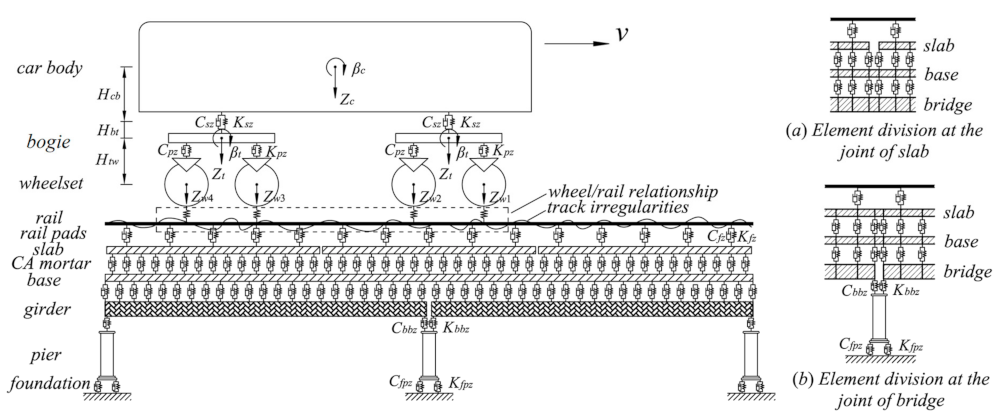
2.1. Model of Vertical Vehicle–Track–Bridge

Bridge deformation has a significant impact especially on the vertical dynamic behavior of vehicles [3]; therefore, in this paper, the vehicle–rail–bridge coupling vertical model was chosen for analysis. The vertical vehicle–track–bridge coupling system comprises three parts: vehicle, track structure, and bridge, which were modeled separately. The vehicle, traveling at speed V, was regarded as a multi-rigid system consisting of a vehicle body, two bogies, four-wheel pairs, and two suspension systems [48,49]; the rail was regarded as a finite-length Euler beam, and the Ritz method was used to solve the differential equations of rail vibration [50]; the track structure–bridge was regarded as a beam unit; based on the principle of the invariant value of total potential energy of an elastic system, the coupled dynamics model of track structure was established [35,51]; vehicle and rail were coupled on the basis of the nonlinear Hertz elastic contact theory [5,8]; the rail and track structure were connected by fasteners, and the fastener system was simulated by spring dampers. The established nonlinear vehicle–track–bridge vertically coupled dynamics model is shown in Figure 1. The explicit–implicit mixed numerical integration mode was used for numerical calculations; the vehicle–track model was analyzed by a novel explicit two-step integration method, which is fast and nonlinearly adaptable; the track–bridge model was solved by the Newmark-β method to ensure the computational stability of the finite element model of the track structure [52].

2.2. Track Irregularity Simulation Method

Track irregularities are stochastic in nature, and the track irregularity power spectrum density (PSD) is generally used to reflect their statistical properties. The PSD can only be directly used in calculation when linear stochastic vibration frequency domain analysis is performed, but in nonlinear stochastic vibration problems, a track stochastic irregularity time-domain sample is also necessary. The commonly used methods for the numerical simulation of a track stochastic irregularity time-domain sample are the triangular series method and the Fourier inversion method [53,54].

Although the number theoretic point selection method can be used to select low-deviation sequences in the stochastic variable selection to reduce the computational convergence time, the low-deviation sequences of stochastic variables selected by the number theoretic point selection method will inevitably be clustered when the stochastic variable dimension is high. In order to reduce the number of stochastic variables required for generating track stochastic irregularities, this paper used the spectral representation random-function method (SRRM) [55] to generate track irregularities time samples, by simulating the generation of track irregularities time samples with a large number of frequency components using two stochastic variables. The track irregularities samples can be expressed as

$$z\left(x\right)={\displaystyle \sum }_{i=1}^N\sqrt{2S_Z\left({\omega }_i\right)\mathsf{\Delta }\omega }·cos\left(2\pi {\omega }_{i}x\right)X_i+sin\left(2\pi {\omega }_{i}x\right)Y_i$$

(1)

where x is the distance in m; $z$ is the track irregularity sample amplitude in mm; ${\omega }_i$ is the spatial frequency component in 1/m; $S_z$ is the track irregularity power spectrum density function, which, in this paper, adopts the Chinese high-speed railway ballastless track spectrum, measured as mm²/(1/m); $X_i$ and $Y_i$ are a set of orthogonal stochastic variables, satisfying, respectively:

$$\left\{\begin{array}{l}E\left[X_i\left]=E\right[Y_i\right]=0\\ E\left[X_i{Y}_j\right]=0\\ E\left[X_i{X}_j\left]=E\right[Y_i{Y}_j\right]={\delta }_{ij}\end{array}\right.$$

(2)

${\delta }_{ij}$ is the Kronecker Delta function.

The Hartley orthogonal basis function was used to construct the orthogonal stochastic variables:

$$\overline{X_i}=cas\left(i{\Theta }_1\right),\overline{Y_i}=cas\left(i{\Theta }_2\right),i=1,2,3,\cdots N$$

(3)

where $cas\left(x\right)=\cos (x)+\sin (x)$; the stochastic variables ${\Theta }_1$ and ${\Theta }_2$ obey a uniform distribution on $\left[0, 2\pi \right]$. The calculation of track irregularity also requires the mapping of the stochastic variable $\left\{X_i,Y_i\right\}$ to $\left\{\overline{X_i},\overline{Y_i}\right\}$. Referring to the high-speed railway ballastless track irregularity power spectrum calculation method in [56], the frequency sampling points were taken as 4096.

2.3. Probability Density Evolution Method for Nonlinear Stochastic Analysis

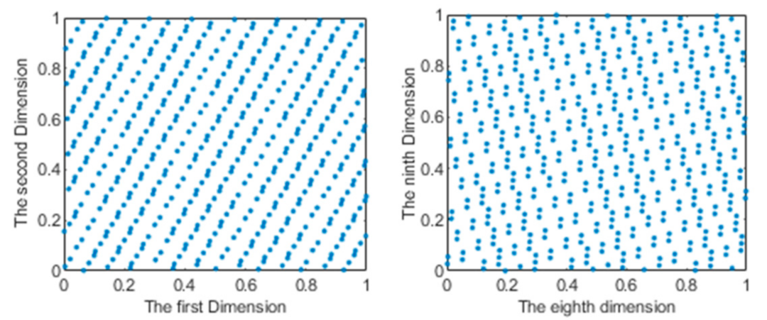
2.3.1. Multi-Distribution Stochastic Sample Selection Method

The stochasticity of the vehicle parameters also needs to be considered in a stochastic analysis because there are differences between vehicles, and the loading condition and service status of the same vehicle can vary [44]. In this paper, the stochasticity of the vehicle parameters acted together with the stochastic track irregularities, and we assumed that the vehicle parameters were normally distributed.

The stochastic parameters in the above-mentioned track irregularity simulation methods has a uniform distribution, but the probability distribution of many stochastic parameters in actual engineering is not unique; distributions like normal distribution are also commonly used. When multiple stochastic factors have to be considered, the selection of stochastic samples and their probabilities given under multiple distributions become the key to the stochastic analysis based on the generalized probability density evolution method [41]. During calculation, the stochastic variable dimension S and the probability distribution of each stochastic variable should be determined, and the set of stochastic variables $\Theta =\left({\Theta }_1, {\Theta }_2, \dots , {\Theta }_s\right)$ should be defined. In this paper, the number of stochastic variables required for the stochastic irregularity simulation was 2, and each variable obeyed a uniform distribution on $\left[0,2\pi \right]$; considering the stochasticity of the vehicle body mass, bogie mass, wheel pair mass, stiffness, and damping of both single-stage suspension and secondary suspension, each parameter obeyed a normal distribution, with a mean E_i and a variation coefficient ${\mu }_i \left(i=1, 2, \dots 7\right)$. After determining the stochastic variables, the number theoretic point selection method was used to select stochastic sample points. The number theoretic point selection, compared with the traditional Monte Carlo method, can generate highly uniformly distributed low-deviation sequences. In this paper, the GP split-circle domain method suggested by Hua Luogeng et al. was used [57], and the uniformity distribution profile of the low-deviation sequences generated by the nine-dimensional GP split-circle domain method is shown in Figure 2. It can be seen that the selected stochastic points in the nine-dimensional GP split-circle domain are distributed uniformly without any cluster phenomenon occurring, so that the calculation accuracy is be influenced by such GP split-circle domain method.

The Voronoi region divide method is used to divide the resulting sample points into representative regions, and the initial probability of each point is equal to the area of its representative region.

2.3.2. Probability Density Evolution Method

The stochasticity of the nonlinear vehicle–track–bridge vertically coupled dynamical system mainly derives from the stochastic irregularity of the track and the stochasticity of the system parameters; then, the system stochastic dynamical equation can be expressed as

$$\left[\mathit{M}\left({\Theta }_m\right)\right]\ddot{\mathit{Z}}\left(t\right)+\left[\mathit{C}\left({\Theta }_c\right)\right]\dot{\mathit{Z}}\left(t\right)+\left[\mathit{K}\left({\Theta }_k\right)\right]\mathit{Z}\left(t\right)=\mathit{F}\left({\Theta }_I,t\right)$$

(4)

where, M, C, K are system mass, damping, and stiffness matrices; ${\Theta }_m,{\Theta }_c,{\Theta }_k$ are the stochastic parameters in the mass, damping, and stiffness matrices; Θ_I is the stochastic parameter of stochastic track irregularity; t is time; $\mathit{Z}\left(t\right)$, $\dot{\mathit{Z}}\left(t\right)$, $\ddot{\mathit{Z}}\left(t\right)$ are the displacement, velocity, and acceleration vectors, respectively; F is the wheel–track excitation caused by stochastic track irregularities.

A system stochastic vector is defined as $\Theta ={\Theta }_m,{\Theta }_c,{\Theta }_k,{\Theta }_I$ under the condition that without the addition of other system stochastic factors during the vehicle operation, the stochasticity of any dynamic response ξ(t) in the coupled vehicle–track–bridge system originates from the stochastic vector $\Theta$, in which all stochastic factors have been included, and the whole system is a probabilistic conservative stochastic system. According to the principle of probability conservation, the probability of the augmented system composed of $\left[\xi \left(t\right), \Theta \right]$ is conserved. Examine the stochastic event $\left(\xi \left(t\right),\Theta \right)\in \left({\Omega }_t\times {\Omega }_{\theta }\right)$, wherein $\Theta$ is the sample realization of the stochastic vector $\Theta$, ${\Omega }_t$ is the distribution space region of $\xi \left(t\right)$ at moment $t$, and ${\Omega }_{\Theta }$ is the distribution space region of $\xi \left(t\right)$ in the sample $\Theta$. At the moment $t+\mathsf{\Delta }t$ after a small time increment $\mathsf{\Delta }t$, the stochastic event evolves as $\left(\xi \left(t+\mathsf{\Delta }t\right),\Theta \right)\in \left({\Omega }_{t+\mathsf{\Delta }t}\times {\Omega }_{\theta }\right)$; obviously, we have

$$P\left\{\left(\xi \left(t\right),\Theta \right)\in \left({\Omega }_t\times {\Omega }_{\theta }\right)\right\}=P\left\{\left(\xi \left(t_{t+\Delta t}\right),\Theta \right)\in \left({\Omega }_t{}_{t+\Delta t}\times {\Omega }_{\theta }\right)\right\}$$

(5)

where P{·} denotes the probability of a stochastic event. Referring to the literature [40,41], the probability density evolution equation can be

$$\frac{\partial p_{{\xi }_{\Theta }}\left(\xi ,\theta ,t\right)}{\partial t}+\dot{\xi }\left(\theta ,t\right)\frac{\partial p_{{\xi }_{\Theta }}\left(\xi ,\theta ,t\right)}{\partial \xi }=0$$

(6)

$\dot{\xi }\left(\theta ,t\right)$ is the velocity of $\dot{\xi }\left(t\right)$ conditional on $\left\{\Theta =\theta \right\}$, namely, $\dot{\xi }\left(t\right)=\partial H\left(\Theta ,t\right)/\partial t$. Its initial condition is:

$${\left.P_{{\xi }_{\Theta }}\left(\xi ,\theta ,t\right)\right|}_{t=0}=\delta \left(\xi -{\xi }_0\right)P_{\Theta }\left(\theta \right)$$

(7)

Solving the above equations to obtain the joint probability density function $P_{\xi \Theta }\left(\xi ,\theta ,t\right)$ and further integrating it over ${\dot{\xi }}_{\Theta }$ to obtain the probability density function of $\dot{\xi }\left(t\right)$, we have:

$$p_{\xi }\left(\xi ,t\right)={\int }_{{\Omega }_{\Theta }}{p}_{{\xi }_{\Theta }}\left(\xi ,\theta ,t\right)d\theta$$

(8)

Since the generalized probability density evolution equation decouples the probability space from the physical space, it is not difficult to obtain the solution to the stochastic nonlinear response of a complex structural system by combining the physical equation with the generalized probability density evolution equation and solving it by numerical methods in sequence.

3. Model Validation

In order to verify the feasibility of the models and methods described in Section 2, the vehicle–track–bridge model and stochastic track irregularity simulation model presented in this paper are compared with the Zhai model [51] in Section 3.1. In Section 3.2, the accuracy of the PDEM method is verified by comparison with the MCM method.

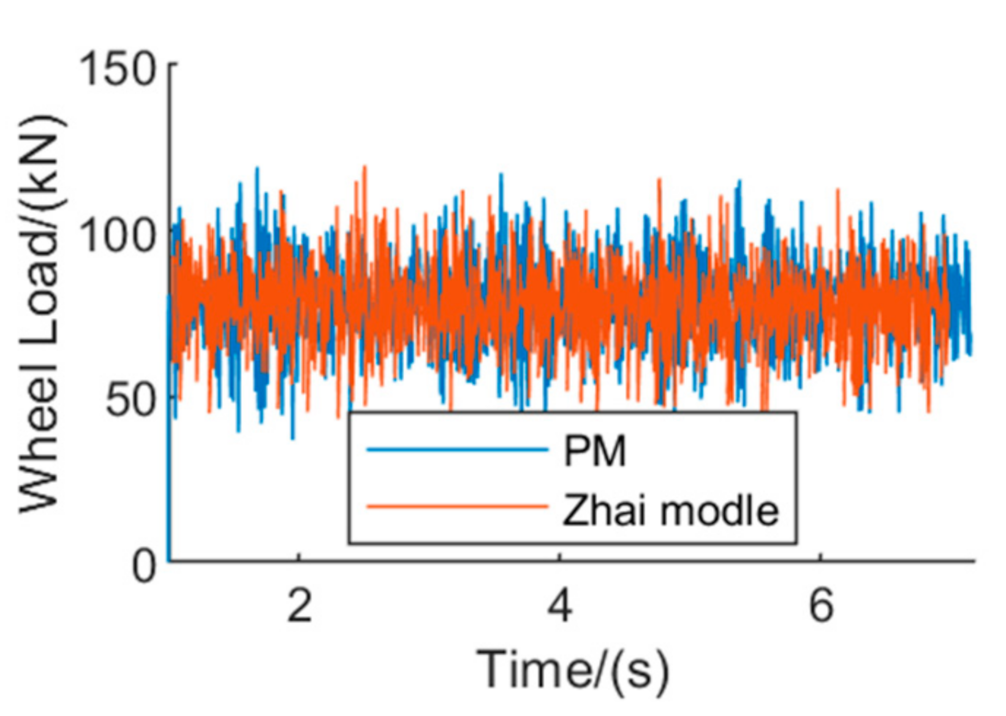
3.1. Coupling Model of Vertical Vehicle–Track–Bridge

The analysis was performed on the Chinese high-speed ballastless railway irregularity spectrum [56], with an irregularity wavelength range of 2–120 m. Figure 3 shows the stochastic irregularity sample in the time domain and frequency spectrum simulated by SRRM. By taking 500 stochastic irregularity samples as a set, the means and standard deviations were compared with those reported in [56] in both time domain and frequency spectrum. The power spectrum of each frequency point in the sample set was tested by ${\chi }^2$ distribution with a significance level of $\alpha =0.05$ and two degrees of freedom, with the Kolmogorov–Smirnov method, verifying the accuracy of the random track irregularities simulated with the present method.

Track irregularities generated by the German railway spectra of low irregularity were used as the excitation input in the vehicle–rail–bridge dynamic model. The ICE3 high-speed train was selected as the vehicle model, and the operation speed was 250 km/h. The parameters are shown in

Table 1. Vehicle parameters.

Parameter	Unit	ICE3	CRH380A
Body mass	kg	48 × 103	33.77 × 103
Bogie mass	kg	3.2 × 103	2.4 × 103
Wheel pair mass	kg	2.4 × 103	1.85 × 103
Body inertia	kg·m2	2.7 × 106	1.65 × 106
Bogie inertia	kg·m2	7.2 × 103	1.31 × 103
Stiffness of single stage suspension	kN/m	1.04 × 103	1.18 × 103
Stiffness of secondary suspension	kN/m	0.4 × 103	0.26 × 103
Damping of single stage suspension	kN·s/m	0	500
Damping of secondary suspension	kN·s/m	0	196
Half of the vehicle’s fixed distance	m	8.6875	8.75
Half of the bogie wheelbase	m	1.25	1.25
Wheel rolling circle radius	m	0.46	0.43

. Taking 10 spans simply supported beams as an example, the length of each span beam was 32.6 m.

Compare the wheel load calculated using the model in this paper (PM) with that in the literature [51], as shown in Figure 4. In [51], the maximum wheel load was 119.78 kN, and the maximum vertical acceleration of the vehicle was 0.51 $\mathrm{m}/{\mathrm{s}}^2$. In PM, the maximum wheel load was 119.26 kN, which was 0.43% less than that in the literature [51]. The results of PM and the classical model differed by less than 10% in the vertical direction, confirming the accuracy of the model developed here.

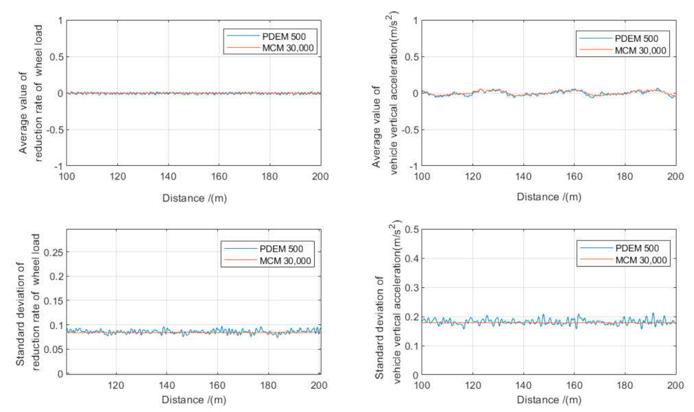
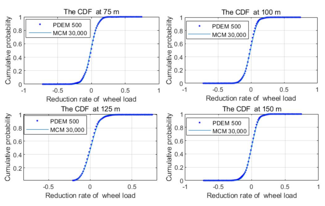
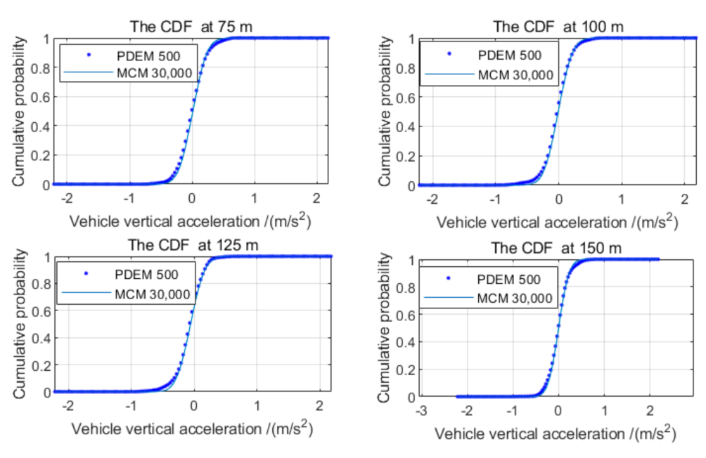
3.2. Probability Density Evolution Method

Taking on-bridge ballastless track as an example, the vehicle dynamics parameters are shown in Table 1, considering the vehicle body, bogie, wheel pair masses, and stiffness and damping of both single-stage suspension and secondary suspension, assuming that each parameter follows a normal distribution. Considering the parameters in the table as the mean value of the vehicle parameters, the variation coefficient was 0.05, also considering the stochasticity of the track irregularity and the vehicle–vertical–safety index, such as body acceleration and reduction rate of wheel load. The comparison of mean values and standard deviations of 500 samples calculated by the generalized probability density evolution method and of 30,000 samples calculated by the Monte Carlo method is shown in Figure 5, and the cumulative probability of indicators at different distances are shown in Figure 6 and Figure 7. It can be seen from Figure 5, Figure 6 and Figure 7 that the mean values, standard deviation, and cumulative probability distribution of the indicators were in good agreement with the results of the Monte Carlo method based on a large number of samples. The calculation method in this paper showed, thus, good accuracy and efficiency.

4. Numerical Results and Discussion

4.1. Comparison of the Influence of Up-Arch and Settlement on Vehicle Operational Safety

For the changes in track irregularities caused by pier settlement and deck variation, assuming the existence of a stochastic variable set Ψ, the track irregularities can be determined by a mapping relationship g(Ψ). The g(Ψ) can be divided into two parts: one is the track irregularity caused by foundation deformation g₁(Ψ). There are many reasons for foundation deformation in ballastless track jointless track on bridge, such as pier settlement, creep camber, deformation caused by temperature, cracking of slab, failure of CA mortar layer, etc. Due to too many influencing factors, the mapping relationship between the foundation deformation and the track irregularity caused by it is not discussed in this paper. Using the method in Refs. [27,28], we described g₁(Ψ) in the form of sine or cosine function. The other component of g(Ψ) is the stochastic irregularity g₂(Ψ) of the original track. The deformation amplitude of the latter is generally smaller than that of the former. For the track irregularity g₁(Ψ), the main determining factors are the length of the deformation section and the amplitude of the irregularity caused by the deformation, which correspond to the wavelength and amplitude of the sine or cosine function, respectively. The track irregularity g₂(Ψ), after the mapping relationship has been determined, still has stochasticity. Since there are stochastic differences in irregularity amplitude even for the same wavelength in the track stochastic irregularity, the effect of infrastructure distortion on track stochastic irregularity is summarized in the stochasticity of track stochastic irregularity. After superimposing g₁(Ψ) and g₂(Ψ) on each other, the track irregularities sample z(x) can be expressed as

$$z\left(x\right)=\left\{\begin{array}{l}\frac{1}{2}a\left(1-\cos \omega x\right)+z\left(x\right)\hspace{0.33em}\hspace{0.33em}\hspace{0.33em}\hspace{0.33em}\hspace{0.33em} (x_b\le x\le x_e)\\ z\left(x\right)\hspace{0.33em}\hspace{0.33em}\hspace{0.33em}\hspace{0.33em}\hspace{0.33em}\hspace{0.33em}\hspace{0.33em}\hspace{0.33em}\hspace{0.33em}\hspace{0.33em}\hspace{0.33em}\hspace{0.33em}\hspace{0.33em}\hspace{0.33em}\hspace{0.33em}\hspace{0.33em}\hspace{0.33em}\hspace{0.33em}\hspace{0.33em}\hspace{0.33em}\hspace{0.33em}\hspace{0.33em}\hspace{0.33em}\hspace{0.33em}\hspace{0.33em}\hspace{0.33em} \left(\mathrm{else}\right) \end{array} \right.$$

(9)

where the spatial frequency $\omega =2\pi /L$, L is the wavelength, $a$ is the amplitude, $\left[x_b,x_e\right]$ is the track irregularity superposition range.

Due to the diverse forms of track distortions, the length and the amplitude of the track irregularity’s influence varies. Studies have shown that in the medium-wave band, at speeds of 300–400 km/h, the most unfavorable wavelengths of irregularity are located at 10–20 m [33]. Here, the harmonic wavelength of 10 m was considered; assuming the foundation settlement was 12 mm, using the Chinese ballastless track irregularity spectrum in [56], and the stochastic irregularity wavelength of 2–120 m, the single sample of track irregularity was calculated as shown in Figure 8.

By using the method of stochastic analysis of a nonlinear vehicle–track–bridge coupled system based on the generalized probability density evolution theory described in this paper, the CRH380A high-speed train was selected as the vehicle model; the probability density evolution process of the reduction rate of wheel load and the acceleration of the vehicle was calculated by considering the travel speed of 350 km/h and the irregularity in Figure 8 as the input excitation, as shown in Figure 9. The reliability of vehicle operating safety with the reduction rate of wheel load of 0.8 as the limit value, and the reliability of vehicle operation safety under such condition was 0.9685.

The maximum possible vehicle acceleration and reduction rate of wheel load in different settlement amplitudes is shown in Figure 10. The safety limits of vehicle acceleration and reduction rate of wheel load were 0.13 g (1.27 m/s²) and 0.8, respectively. Obviously, the reduction rate of wheel load was more stringent as a standard, so it was uniformly selected as the operation safety and reliability index.

The most common foundation deformation of the track can be roughly divided into settlement and up-arch. Considering only the influence of foundation deformation on track irregularity, in the case of 12 mm up-arch, the equiprobability curve of reduction rate of wheel load probability density is shown in Figure 11, and the reliability of vehicle-vertical safety was 0.9978, as shown in Figure 12.

It can be seen that the settlement was lowered with respect to the up-arch by 0.0293, which is about 3.02%, and this indicated that the foundation settlement was more unfavorable to the vehicle vertical safety. The reason for this are varied, for example, different states of the track structure support will have an influence in different degrees. Only the influence of foundation deformation on track irregularity was considered in this paper, while the influence on the other parts of the track structure was not considered.

4.2. The Impact of Stochastic Vehicle Parameters on the Safety of Vehicle Operation

There are variations among different vehicles, and the same vehicle can vary in loading and service status. In this paper, we propose to use variation coefficients to describe such changes. The vehicle parameters include the masses of the vehicle body, bogies, and wheel pairs, as well as the stiffness and damping of the single-stage suspension and secondary suspension. In the case of a 12 mm settlement, and assuming a VCVP od 0.2, the equiprobability curve of the reduction rate of wheel load at the operation speed of 350 km/h is shown in Figure 13.

The probability density of the reduction rate of wheel load with different variation coefficients of vehicle parameters at the operation speed of 350 km/h is shown in Figure 14; with the increase of the variation coefficient, the peak of the probability density gradually decreases and shifts to the left, but its variation range increases.

The variation of the overload probability of the reduction rate of wheel load with the VCVP is shown in Figure 15, and the relationship therebetween exhibits an obvious nonlinearity; with the increase of the VCVP, the overload probability gradually increases. Compared with the VCVP of 0, the overload probability increased by 6.01% when the VCVP was 0.1; when the vehicle parameter variation coefficient was 0.2, the overload probability increased by 14.60%.

The variation coefficient of the reduction rate of wheel load as the function of the variation coefficient of the vehicle parameters is shown in Figure 16 at the position of the maximum reduction rate of wheel load. The variation coefficient of the reduction rate of wheel load exhibited a nonlinear increase with the increase of the VCVP, which also means an increase of its dispersion and unpredictability. Compared with the case when the VCVP was 0, the variation coefficient of the reduction rate of wheel load increased by 0.049, and when the VCVP was 0.1 and 0.2, respectively, it increased by 0.189, which shows that the stochasticity of the vehicle parameters has a significant impact on the safety of vehicle operation.

4.3. Comprehensive Influence of the Amplitude, Speed and VCVP on Operation Safety

At present, the maximum operating speed of high-speed railways in China has reached 350 km/h, and research is undergoing to develop the technology for an operating speed above 350 km/h. Using the method of the impact of infrastructure disruption on the vehicle operating safety based on the stochastic analysis in this paper, taking the example of 10 m as harmonic irregularity wavelength and 2–120 m as stochastic irregularity wavelength, calculating different VCVP and the amplitude of different harmonic irregularity when the operating speed was in the range of 350–450 km/h, we obtained the calculation results of reliability shown in Figure 17.

As can be seen in Figure 17, the stochasticity of the vehicle parameters is a factor that must be considered in the stochastic analysis of vehicle–track–bridge coupled dynamics. The reliability of vehicle vertical safety decreases gradually with the increase of vehicle operation speed, irregularity amplitude, and VCVP. It can be observed in the figures that at the speeds of 400 km/h, 425 km/h, 450 km/h, the degree of influence on the reliability of vehicle vertical safety was higher with respect to the change of track irregularity amplitude than with respect to the change of VCVP. In contrast, when the operation speed was not less than 425 km/h and the amplitude of the foundation settlement was greater than 10 mm, the variation coefficient of the vehicle parameters might increase, as well as the reliability of vehicle vertical safety, which may due to the fact that the vehicle parameters could be optimized at high operation speed. In addition, at an operation speed higher than 375 km/h, when the irregularity amplitude caused by foundation deformation is greater than 6 mm, the attenuation of reliability increased; so, in the construction of high-speed railways and their maintenance and reparation, it is important to ensure that the irregularity amplitude caused by foundation deformation is less than 6 mm.

Because of the lack of research on vehicle parameters stochasticity and their distribution, a quantitative analysis per se is still difficulty, and in the case of large variation coefficients, the vehicle needs maintenance; so in this paper, only

Table 2. Reliability of vehicle vertical safety at 350 km/h and above without considering stochastic vehicle parameters.

	Speed (km/h)	350	375	400	425	450
Amplitude
5 mm		1.0000	1.0000	0.9997	0.9959	0.9925
6 mm		1.0000	1.0000	0.9973	0.9929	0.9826
7 mm		1.0000	0.9993	0.9966	0.9745	0.9426
8 mm		1.0000	0.9973	0.9798	0.9430	0.8733
9 mm		1.0000	0.9898	0.9487	0.8857	0.7641
10 mm		1.0000	0.9717	0.9055	0.8144	0.6511
11 mm		0.9974	0.9462	0.8407	0.6426	0.4604
12 mm		0.9685	0.8777	0.6864	0.4763	0.3224

The dyed part is higher than the safety limit.

lists the different settlement amplitudes when the VCVP was not considered.

Table 3. Reliability of vehicle vertical safety at 350 km/h and above for VCVP of 0.1.

	Speed (km/h)	350	375	400	425	450
Amplitude
5 mm		1.0000	0.9985	0.9945	0.9788	0.9718
6 mm		1.0000	0.9962	0.9816	0.9775	0.9399
7 mm		0.9954	0.9928	0.9815	0.9372	0.9088
8 mm		0.9859	0.9746	0.9392	0.8840	0.8333
9 mm		0.9759	0.9462	0.8868	0.8255	0.7565
10 mm		0.9542	0.9103	0.8378	0.7564	0.6670
11 mm		0.9391	0.8795	0.7727	0.6559	0.5461
12 mm		0.9181	0.7967	0.6827	0.5488	0.4499

The dyed part is higher than the safety limit.

lists the different settlement amplitudes of the reliability of vehicle vertical safety when the VCVP was 0.1. Considering Figure 17 together with Table 2 and Table 3, it can be observed that for speeds of 350 km/h and 375 km/h, the degree of influence on the reliability of vehicle vertical safety was higher with respect to the change of VCVP than with respect to the change of track irregularity amplitude.

5. Conclusions

In this paper, harmonic irregularity was used to describe the track irregularities caused by infrastructure disruptions; the effect of disruptions wis superposed on the stochastic track irregularities, and the vehicle vertical safety was evaluated based on the stochastic analysis of a nonlinear vehicle–track–bridge coupled system.

(1)

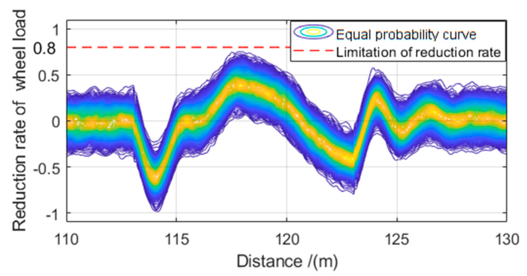
The vertical acceleration at the center plate and the dynamic reduction rate of wheel load under the influence of different foundation deformation amplitudes were calculated. Compared with the limit of 0.13 g of the vertical acceleration, the limit of 0.8 of the reduction rate of wheel load is more strict.

(2)

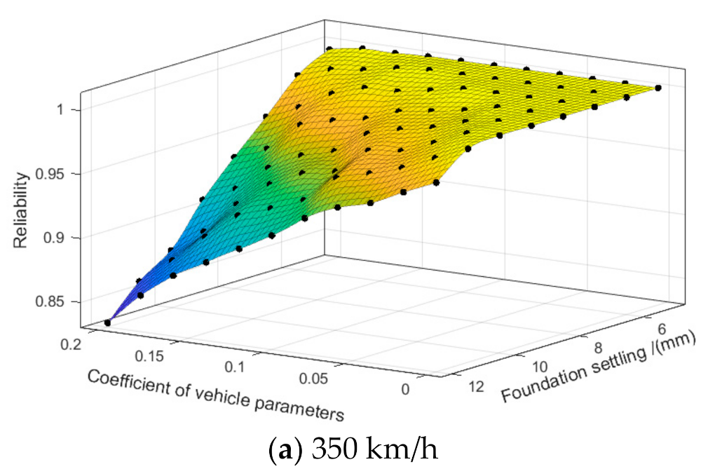
From the point of view of reliability, settlement is more harmful to vehicle safety than up-arch. In the case of a wavelength of 10 m, the amplitude is 12 mm, VCVP is 0, and the operation speed is 350 km/h; the reliability of operation safety in settlement compared to the up-arch was reduced by 0.0293, corresponding to about 3.02%. With the increase of VCVP, the influence of settlement was more significant.

(3)

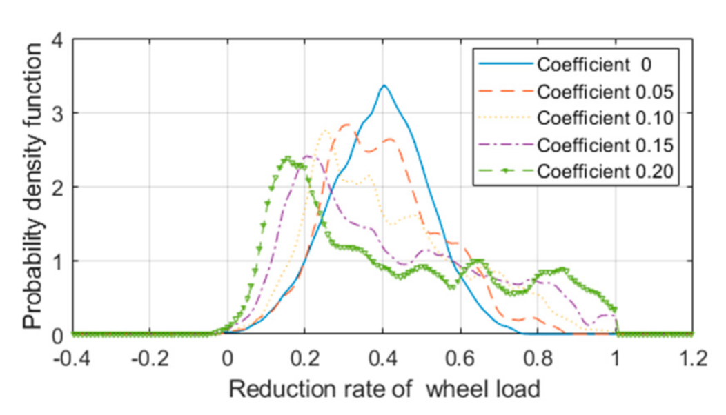
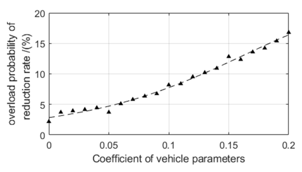
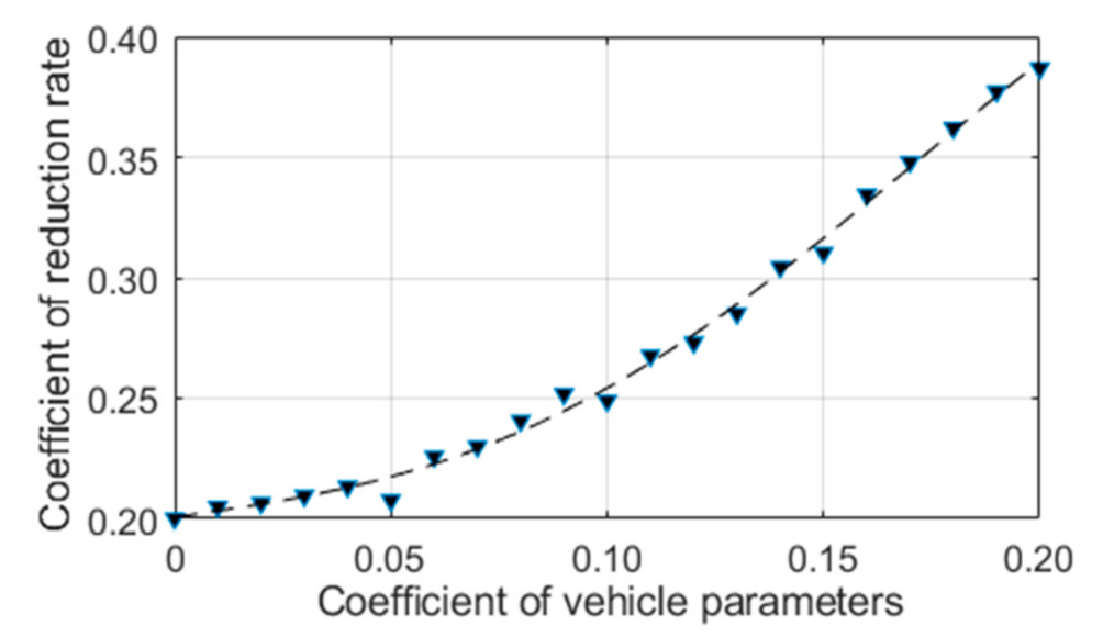
The stochasticity of the vehicle parameters has a non-negligible impact on the vehicle vertical safety, and the increase of the dispersion of vehicle parameters will gradually reduce the safety of vehicle operation. Regardless of the influence of the stochasticity of the vehicle parameters (speed 350 km/h), a deformation amplitude of 10 mm will not affect the reliability of operation safety. However, considering the certain dispersion of vehicle parameters, a deformation amplitude greater than 6 mm will affect the operation reliability.

(4)

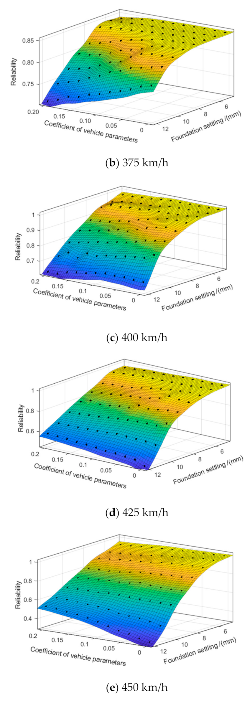
When the operation speed is higher than 375 km/h, the amplitude of track irregularities will have a greater impact on the safety of vehicle operation. Therefore, in the design, construction, and operation of higher-speed trains, it is necessary to adopt more stringent standards for bridge structure deformation. In addition, it can be seen from the calculation results that there is a better combination of vehicle parameters at higher driving speeds.

References

- Zhai, W.; Han, Z.; Chen, Z.; Ling, L.; Zhu, S. Train–track–bridge dynamic interaction: A state-of-the-art review. Veh. Syst. Dyn. 2019, 57, 984–1027. [Google Scholar] [CrossRef] [Green Version]
- Chen, X.; Deng, X.; Xu, L. A Three-Dimensional Dynamic Model for Railway Vehicle-Track Interactions. J. Comput. Nonlinear Dyn. 2018, 13, 071006. [Google Scholar] [CrossRef]
- Chen, Z.; Zhai, W.; Cai, C.; Sun, Y. Safety threshold of high-speed railway pier settlement based on train-track-bridge dynamic interaction. Sci. China-Technol. Sci. 2015, 58, 202–210. [Google Scholar] [CrossRef]
- Chen, Z.; Zhai, W.; Tian, G. Study on the safe value of multi-pier settlement for simply supported girder bridges in high-speed railways. Struct. Infrastruct. Eng. 2018, 14, 400–410. [Google Scholar] [CrossRef]
- Chen, Z.; Zhai, W.; Yin, Q. Analysis of structural stresses of tracks and vehicle dynamic responses in train-track-bridge system with pier settlement. Proc. Inst. Mech. Eng. Part F-J. Rail Rapid Transit. 2018, 232, 421–434. [Google Scholar] [CrossRef]
- Chen, Z.; Xu, L.; Zhai, W. Investigation on the Detrimental Wavelength of Track Irregularity for the Suspended Monorail Vehicle System. In Railway Development, Operations, and Maintenance: Proceedings of the First International Conference on Rail Transportation 2017 (Icrt 2017); Zhai, W.M., Wang, K.C.P., Eds.; American Society of Civil Engineers: New York, NY, USA, 2018; pp. 161–168. Available online: https://www.webofscience.com/wos/alldb/summary/38e078ea-3e23-440c-a0e1-08e2cc564f9f-1f698566/relevance/1 (accessed on 18 January 2022).
- Zhai, W.; Wang, S.; Zhang, N.; Gao, M.; Xia, H.; Cai, C.; Zhao, C. High-speed train–track–bridge dynamic interactions—Part II: Experimental validation and engineering application. Int. J. Rail Transp. 2013, 1, 25–41. [Google Scholar] [CrossRef]
- Zhai, W.; Xia, H.; Cai, C.; Gao, M.; Li, X.; Guo, X.; Zhang, N.; Wang, K. High-speed train–track–bridge dynamic interactions—Part I: Theoretical model and numerical simulation. Int. J. Rail Transp. 2013, 1, 3–24. [Google Scholar] [CrossRef]
- Zeng, Z.-P.; Xiao, Y.-C.; Wang, W.-D.; Huang, X.-D.; Du, X.-G.; Liu, L.-L.; Victor, J.E.; Xie, Z.-L.; Yuan, Y.; Wang, J.-D. The Influence of Track Structure Parameters on the Dynamic Response Sensitivity of Heavy Haul Train-LVT System. Appl. Sci. 2021, 11, 11830. [Google Scholar] [CrossRef]
- Saramago, G.; Montenegro, P.A.; Ribeiro, D.; Silva, A.; Santos, S.; Calçada, R. Experimental Validation of a Double-Deck Track-Bridge System under Railway Traffic. Sustainability 2022, 14, 5794. [Google Scholar] [CrossRef]
- Zhao, G.; Cai, X.; Liu, W.; Wang, T.; Wang, T. Mechanical Properties and Structural Optimization of Continuous Welded Rail on Super-Long-Span Suspension Bridges for High-Speed Railway. Appl. Sci. 2021, 12, 305. [Google Scholar] [CrossRef]
- Sakhare, A.; Farooq, H.; Nimbalkar, S.; Dodagoudar, G.R. Dynamic Behavior of the Transition Zone of an Integral Abutment Bridge. Sustainability 2022, 14, 4118. [Google Scholar] [CrossRef]
- Zhang, T.; Jin, T.; Luo, J.; Zhu, S.; Wang, K. Stochastic Analysis on the Resonance of Railway Trains Moving over a Series of Simply Supported Bridges. Shock. Vib. 2021, 2021, e1491207. [Google Scholar] [CrossRef]
- Luo, J.; Zeng, Z. A novel algorithm for longitudinal track-bridge interactions considering loading history and using a verified mechanical model of fasteners. Eng. Struct. 2019, 183, 52–68. [Google Scholar] [CrossRef]
- Chang, W.; Cai, X.; Wang, Q.; Tang, X.; Sun, J.; Yang, F. The Influence of Track Irregularity in Front of the Turnout on the Dynamic Performance of Vehicles. Appl. Sci. 2022, 22, 4169. [Google Scholar] [CrossRef]
- Gu, Q.; Pan, J.; Liu, Y.; Fu, M.; Zhang, J. An Effective Tangent Stiffness of Train–Track–Bridge Systems Based on Artificial Neural Network. Appl. Sci. 2022, 12, 2735. [Google Scholar] [CrossRef]
- Dou, Y.; Wang, P.; Ding, W.; Wang, S.; Wei, K. Effect of viscoelastic-plastic dynamic properties of rail pads on curved rail dynamic characteristics based on the modified SEM-SM hybrid method. Veh. Syst. Dyn. 2022, 1–25. [Google Scholar] [CrossRef]
- Luo, J.; Zhu, S.; Zhai, W. Development of a track dynamics model using Mindlin plate theory and its application to coupled vehicle-floating slab track systems. Mech. Syst. Signal Process. 2020, 140, 106641. [Google Scholar] [CrossRef]
- Luo, J.; Zhu, S.; Zhai, W. An advanced train-slab track spatially coupled dynamics model: Theoretical methodologies and numerical applications. J. Sound Vib. 2021, 501, 116059. [Google Scholar] [CrossRef]
- Luo, J.; Zhu, S.; Zhai, W. Exact closed-form solution for free vibration of Euler-Bernoulli and Timoshenko beams with intermediate elastic supports. Int. J. Mech. Sci. 2022, 213, 106842. [Google Scholar] [CrossRef]
- Luo, J.; Zhu, S.; Zhai, W. Formulation of curved beam vibrations and its extended application to train-track spatial interactions. Mech. Syst. Signal Process. 2022, 165, 108393. [Google Scholar] [CrossRef]
- Chiacchiari, L.; Loprencipe, G. Measurement methods and analysis tools for rail irregularities: A case study for urban tram track. J. Mod. Transp. 2015, 23, 137–147. [Google Scholar] [CrossRef]
- Chiacchiari, L.; Thompson, D.; Squicciarini, G.; Ntotsios, E.; Loprencipe, G. Rail roughness and rolling noise in tramways. J. Phys. Conf. Ser. 2016, 744, 012147. [Google Scholar] [CrossRef] [Green Version]
- Sheng, X.; Jones, C.J.C.; Thompson, D.J. A theoretical model for ground vibration from trains generated by vertical track irregularities. J. Sound Vib. 2004, 272, 937–965. [Google Scholar] [CrossRef]
- Grassie, S.L. Rail corrugation: Advances in measurement, understanding and treatment. Wear 2005, 258, 1224–1234. [Google Scholar] [CrossRef]
- Grassie, S.L. Squats and squat-type defects in rails: The understanding to date. Proc. Inst. Mech. Eng. Part F J. Rail Rapid Transit 2012, 226, 235–242. [Google Scholar] [CrossRef]
- Cai, C.B.; Zhai, W.M.; Wang, Q.C. Study on Allowable Safety Criterion of Track Geometric Irregularities. J. China Railw. Soc. 1995, 17, 82–87. [Google Scholar]
- Zhai, W. Vehicle-Track-Coupled Dynamics, 3rd ed.; Science Press: Beijing, China, 2007. [Google Scholar]
- Chen, G.; Zhai, W.M.; Zuo, H.F. Safety Management of Track Irregularities of 250 km/h High-Speed Railway. J. Southwest Jiaotong Univ. 2001, 36, 495–499. [Google Scholar]
- Li, M.H.; Li, L.L.; He, X.Y. Research on the Control of Track Irregularity of High-speed Railway. J. Raiway Eng. Soc. 2009, 26, 26–30. [Google Scholar]
- Tian, G.; Gao, J.M.; Zhai, W.M. Comparative Analysis of Track Irregularity Management Standards for High-speed Railways. J. China Railw. Soc. 2015, 37, 64–71. [Google Scholar]
- Tian, G.; Gao, J.M.; Zhai, W.M. A Method for Estimation of Track Irregularity Limits Using Track Irregularity Power Spectrum Density of High-speed Railway. J. China Railw. Soc. 2015, 37, 83–90. [Google Scholar]
- Gao, J.M.; Zhai, W.M.; Wang, K.Y. Study on Sensitive Wavelengths of Track Irregularities in High-speed Operation. J. China Railw. Soc. 2012, 34, 83–88. [Google Scholar]
- Chen, Z.; Bi, L.; Zhao, J. Comparison of single-pier settlement model and multi-pier settlement model in solving train-track-bridge interaction. Veh. Syst. Dyn. 2021, 59, 1484–1508. [Google Scholar] [CrossRef]
- Zeng, Z.; Yu, Z.; Zhao, Y.-G.; Xu, W.; Chen, L.-K.; Lou, P. Numerical Simulation of Vertical Random Vibration of Train-Slab Track-Bridge Interaction System by PEM. Shock. Vib. 2014, 2014, e304219. [Google Scholar] [CrossRef] [Green Version]
- Zeng, Z.; He, X.; Zhao, Y.; Yu, Z.; Chen, L.; Xu, W.; Lou, P. Random vibration analysis of train-slab track-bridge coupling system under earthquakes. Struct. Eng. Mech. 2015, 54, 1017–1044. [Google Scholar] [CrossRef]
- Zeng, Z.-P.; Liu, F.-S.; Lou, P.; Zhao, Y.-G.; Peng, L.-M. Formulation of three-dimensional equations of motion for train-slab track-bridge interaction system and its application to random vibration analysis. Appl. Math. Model. 2016, 40, 5891–5929. [Google Scholar] [CrossRef]
- Wan, H.-P.; Ni, Y.-Q. An efficient approach for dynamic global sensitivity analysis of stochastic train-track-bridge system. Mech. Syst. Signal Process. 2019, 117, 843–861. [Google Scholar] [CrossRef]
- Li, J. A PDEM-based perspective to engineering reliability: From structures to lifeline networks. Front. Struct. Civ. Eng. 2020, 14, 1056–1065. [Google Scholar] [CrossRef]
- Li, J.; Chen, J. The probability density evolution method for analysis of dynamic nonlinear response of stochastic structures. Chin. J. Theor. Appl. Mech. 2003, 35, 716–722. [Google Scholar]
- Li, J.; Chen, J. Some research progress of probability density evolution theory. Appl. Math. Mech. 2017, 38, 32–43. [Google Scholar]
- Yu, Z.; Mao, J. Probability analysis of train-track-bridge interactions using a random wheel/rail contact model. Eng. Struct. 2017, 144, 120–138. [Google Scholar] [CrossRef]
- Yu, Z.; Mao, J.; Tan, S.; Zeng, Z. The Stochastic Analysis of the Track-bridge Vertical Coupled Vibration with Random Train Parameters. J. China Railw. Soc. 2015, 37, 97–104. [Google Scholar]
- Mao, J.; Yu, Z.; Xiao, Y.; Jin, C.; Bai, Y. Random dynamic analysis of a train-bridge coupled system involving random system parameters based on probability density evolution method. Probabilistic Eng. Mech. 2016, 46, 48–61. [Google Scholar] [CrossRef]
- Xu, L.; Zhai, W.; Gao, J. A probabilistic model for track random irregularities in vehicle/track coupled dynamics. Appl. Math. Model. 2017, 51, 145–158. [Google Scholar] [CrossRef]
- Liu, F.-S.; Zeng, Z.-P.; Wang, W.-D.; Shuaibu, A.A. Stochastic Analysis of Nonlinear Vehicle-Track Coupled Dynamic System and Its Application in Vehicle Operation Safety Evaluation. Shock. Vib. 2019, 2019, e3236093. [Google Scholar] [CrossRef]
- Liu, F.; Zeng, Z.; Guo, W.; Zhu, Z. Random vibration analysis of vehicle-track-bridge vertical coupling system considering wheel-rail nonlinear contact. J. Vib. Eng. 2020, 33, 139–148. [Google Scholar]
- Zhai, W. Vehicle–Track Coupled Dynamics: Theory and Applications; Springer: Singapore, 2020. [Google Scholar] [CrossRef]
- Zhai, W.; Wang, K.; Cai, C. Fundamentals of vehicle–track coupled dynamics. Veh. Syst. Dyn. 2009, 47, 1349–1376. [Google Scholar] [CrossRef]
- Zhai, W.M.; Cai, C.B.; Guo, S.Z. Coupling Model of Vertical and Lateral Vehicle/Track Interactions. Veh. Syst. Dyn. 1996, 26, 61–79. [Google Scholar] [CrossRef]
- Zhai, W.M.; Xia, H. Train-Track-Bridge Dynamic Interaction:Theory and Engineering Application; Science Press: Beijing, China, 2011. [Google Scholar]
- Zhai, W. Two simple fast integration methods for large-scale dynamic problems in engineering. Int. J. Numer. Methods Eng. 1996, 39, 4199–4214. [Google Scholar] [CrossRef]
- Wang, F.; Zhou, J.; Ren, L. Analysis on track spectrum density for dynamic simulations of high-speed vehicles. J. China Railw. Soc. 2002, 24, 21–27. [Google Scholar]
- Liu, Y.; Li, F.; Huang, Y. Numerical Simulation Methods of Railway Track Irregularities. J. Traffic Transp. Eng. 2006, 6, 29–33. [Google Scholar]
- Liu, Z.; Liu, W.; Peng, Y. Random function based spectral representation of stationary and non-stationary stochastic processes. Probabilistic Eng. Mech. 2016, 45, 115–126. [Google Scholar] [CrossRef]
- TB/T 3352-2014; PSD of Ballastless Track Irregularities of High-Speed Railway. National Railway Administration: Beijing, China, 2014.
- Hua, L.G.; Wang, Y.; Pei, D.Y. On the independent unit system of the sub-circular domain. Chin. J. Nat. 1978, 1, 6. [Google Scholar]