Development of the Dynamic Stiffness Method for the Out-of-Plane Natural Vibration of an Orthotropic Plate

Abstract

In this present paper, the dynamic stiffness method (DSM) was formulated to investigate the out-of-plane natural vibration of a thin orthotropic plate using the classical plate theory (CPT). Hamilton’s principle was implemented to derive the governing differential equation of motion for free vibration of the orthotropic plate for Levy-type boundary conditions. The Wittrick–Williams (W–W) algorithm was used as a solution technique to compute the natural frequencies of a thin orthotropic plate for different boundary conditions, aspect ratios, thickness ratios, and modulus ratios. The obtained results are compared with the results by the finite element method using commercial software (ANSYS and those available) in the published literature. The presented results by the dynamic stiffness method can be used as a benchmark solution to compare the natural frequencies of orthotropic plates.

1. Introduction

A rectangular orthotropic plate has many applications in designing different components in the engineering field, such as aerospace, mechanical, and civil. The orthotropic response of a given material is due to the existence of its constitutive relations. Various composite plates have been modeled analytically as orthotropic plates in recent years. So, one should have knowledge of the free vibration of such structures for efficient dynamic structural analyses. Starting from the earlier works on natural vibration of the plate by Rayleigh [1] and Ritz [2], the past few decades have witnessed different numerical and analytical methods, such as the Kantorovich method, the superposition method, the Rayleigh–Ritz method, and the iterative reduction method, for the investigation of natural vibrations of rectangular orthotropic plates [3,4,5,6,7,8,9,10,11,12,13,14,15,16,17,18,19,20]. The usually adopted finite element method (FEM) has also proved its popularity in the dynamic analysis of orthotropic rectangular plates [21,22,23]. However, the main drawback of traditional FEM and other approximate methods is the discretization technique of the given structure, which depends on the number of elements taken. The dynamic stiffness method (DSM) provides accurate results independent of the number of elements implemented in the investigation. The DSM has proven its efficiency in the dynamic analysis of bars, beams, rings, and shells [24,25,26,27,28,29,30,31], and the W–W algorithm [24,25,26,27,28] is implemented as a solution technique to the final dynamic stiffness matrix to find out the natural vibration frequencies of beams. Wittrick and Williams [32] are probably the earliest researchers who developed DSM for isotropic simply supported plates, applying CPT. Boscolo and Banerjee extended the DSM and applied the first-order deformation theory (FSDT) for isotropic [33] and composite plates [34,35]. Fazzolari et al. [36] further formulated the DSM for rectangular anisotropic plates using the higher shear deformation theory (HSDT) with the W–W algorithm. Further, Boscolo and Banerjee [37] developed DSM by applying the sophisticated layer-wise first-order theory to investigate laminated composite plates. Continuing this work, Banerjee et al. [38] developed an exact dynamic stiffness (DS) matrix for an isotropic rectangular plate. Thinh et al. [39] used DSM for free vibration analyses of thick composite plates resting on non-homogeneous foundations. Recently, Danilovic et al. developed DSM for an isotropic rectangular plate with arbitrary boundary conditions undergoing in-plane free vibration [40], which was further exploited for out-of-plane free vibration of the rectangular Mindlin plate element [41] and later on for isotropic plate assemblies [42]. Ghorbel et al. formulated DSM for both out-of-plane [43] and in-plane [44] free vibrations of the rectangular orthotropic plate, taking advantage of the symmetry and Gorman-type decomposition of the free boundary conditions. Kumar et al. [45] developed DSM for analyzing the free vibration response of the functionally-graded material plate using the classical plate theory with the physical neutral surface concept. Chauhan et al. [46] used the classical plate theory to formulate a dynamic stiffness matrix to compute the natural frequencies of the rectangular plate with the considered Levy-type boundary conditions. Moreover, Liu and Banerjee developed an exact spectral–dynamic stiffness method (S–DSM), which combines the spectral method with classical DSM for free vibration analyses of orthotropic composite plates and their assemblies [47,48] and, subsequently, for isotropic rectangular plates [49] with arbitrary boundary conditions.

This work reports the out-of-plane free vibration response of a thin rectangular orthotropic plate for Levy-type boundary conditions based on CPT using the exact DSM method with the Wittrick–Williams algorithm. The explicit terms of the DS matrix and natural frequencies of the orthotropic plate by the Wittrick–Williams algorithm for different boundary conditions, aspect ratios, thickness ratios, and modulus ratios are reported and compared with the available published literature and finite element method. The remaining portion of the present work can be described as follows: After the introduction, Section 2 explains the main contributions of the present study. In Section 3, the mathematical formulation of the orthotropic plate with material property is reported. Here, the fundamental principle of mathematical modeling of DSM and the motion governing equation of the orthotropic plate, formulated using Hamilton’s principle, are highlighted. Along with this, a dynamic stiffness matrix was generated, and the W–W algorithm was used to investigate the natural frequencies of the orthotropic plate. Section 4 described the natural frequency results highlighting the effects of geometric parameters on the natural frequency of the orthotropic plate. Section 5 presents the conclusions of the present study.

2. Contributions and Relevant Scope of Present Work

In the present study, the natural vibration response in the transverse direction of the orthotropic plate was investigated. The classical plate theory explains the plate displacement component or kinematic variables. Hence, the effect of shear deformation of the plate can be neglected, and the present work is mainly focused on thin orthotropic plates. The Levy-type solution was applied where two opposite sides of the plate were simply supported, and the other two sides had arbitrary conditions (free, clamped, and simply supported). In the present study’s relevant scopes and limitations, the paper’s main contributions can be explained as follows:

• The DSM was formulated to investigate the natural vibration response of thin orthotropic plates.
• The W–W algorithm was applied to compute the natural frequency of the orthotropic plate.
• The DSM results were compared with the published literature and the finite element method.
• A new set of DSM results is reported for different aspect ratios, thickness ratios, and modulus ratios, which may be used as benchmark solutions for comparison.

3. Mathematical Formulation

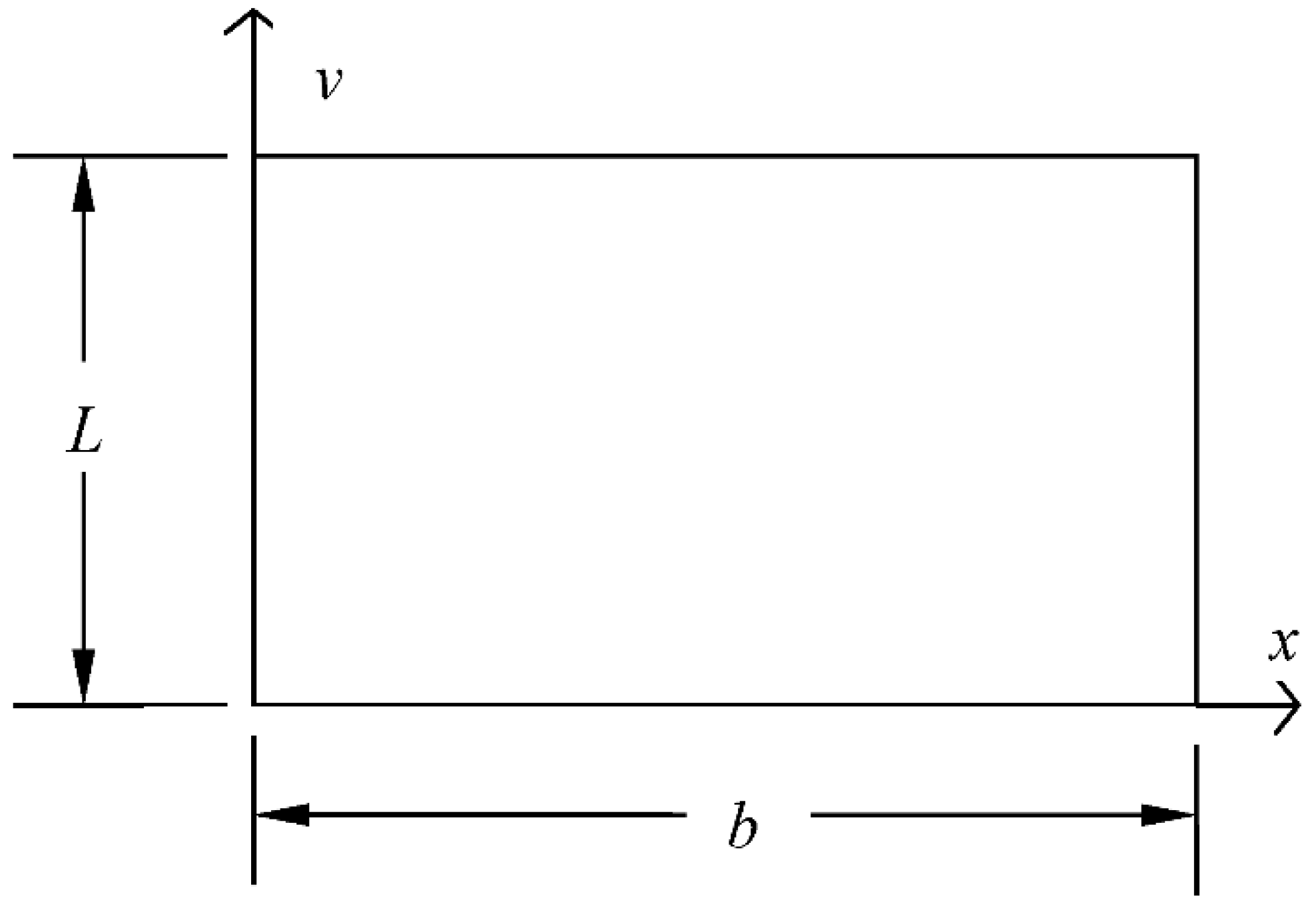
3.1. Description of Geometrical Property

Figure 1 shows the coordinate system of a thin orthotropic plate where the plate length is $L$, with $b,$ and thickness is $h.$ The Levy-type solution is applied where two opposite edges are simply supported along the y-axis (i.e., along the edges $y=0,$ and $y=L$), while the other two edges may be free $\left(F\right)$, simply supported $\left(S\right)$, or clamped $\left(C\right)$, as represented in Figure 2. The material orthotropic axes of the plate are parallel in the directions of x and y.

Applying the CPT assumption, the transverse displacements of an arbitrary point of the plate are expressed by Equation (1).

$$u=\left\{\begin{array}{c}u\left(x,y,z\right)\\ v\left(x,y,z\right)\\ w\left(x,y,z\right)\end{array}\right\}$$

$$u=\left\{\begin{array}{c}-z\frac{\partial w^0}{\partial x}\\ -z\frac{\partial w^0}{\partial y}\\ w^0\left(x,y\right)\end{array}\right\}$$

(1)

where the displacement components of the plate are represented by $u,v,w$ in $x$, $y$, $z$ directions, respectively, and $\frac{\partial w^0}{\partial x}={\varnothing }_y$, $\frac{\partial w^0}{\partial y}={\varnothing }_x$ represents the rotational displacements of the $x$ and $y$ axes at the plate middle surface, respectively. $w^0$ represents the thickness (transverse) displacement in the z-direction.

In the case of orthotropic plates, the orientation of the constitutive material is such that orthotropic axes 1 and 2 are equal to axes x and y, respectively, and the material constants, ${\mathcal{Q}}_{ij}$ are given by Equation (2).

$$\left\{{\mathcal{Q}}_{ij}\right\}=\left\{\begin{array}{c}{\mathcal{Q}}_{11}=\frac{E_1}{\left(1-{\vartheta }_{12}{\vartheta }_{21}\right)}\\ {\mathcal{Q}}_{22}=\frac{E_2}{\left(1-{\vartheta }_{12}{\vartheta }_{21}\right)}\\ {\mathcal{Q}}_{12}=\frac{{\vartheta }_{12}{E}_1}{\left(1-{\vartheta }_{12}{\vartheta }_{21}\right)}\\ {\mathcal{Q}}_{66}=G_{12}\end{array}\right\}$$

(2)

where $E_1$, $E_2$ are Young’s moduli, along with the orthotropic directions 1 and 2, respectively; ${\vartheta }_{12}$, ${\vartheta }_{21}$ are major and minor Poisson’s ratios, and $G_{12}$ is the shear modulus [43].

3.2. Equations of Motion

The well-known Hamilton’s principle is used to derive the governing differential equation for the natural vibration of the orthotropic plate based upon CPT as given by Equation (3).

$$D_x\frac{{\partial }^4{w}^0}{\partial x^4}+D_{xy}\frac{{\partial }^4{w}^0}{\partial x^2\partial y^2}+D_y\frac{{\partial }^4{w}^0}{\partial y^4}=\rho h\frac{{\partial }^2{w}^0}{\partial t^2}$$

(3)

where the mass density and thickness of the orthotropic plate are represented by $\rho$ and $h$, respectively.

$D_x$, $D_y$, and $D_{xy}$ are flexural rigidities, which are given by Equation (4).

$$\begin{gathered} D_x=-\frac{h^3}{12}{\mathcal{Q}}_{11} \\ {D}_{xy}=-\frac{h^3}{6}{\mathcal{Q}}_{12}-4\frac{h^3}{12}{\mathcal{Q}}_{66} \\ {D}_y=-\frac{h^3}{12}{\mathcal{Q}}_{22} \end{gathered}$$

(4)

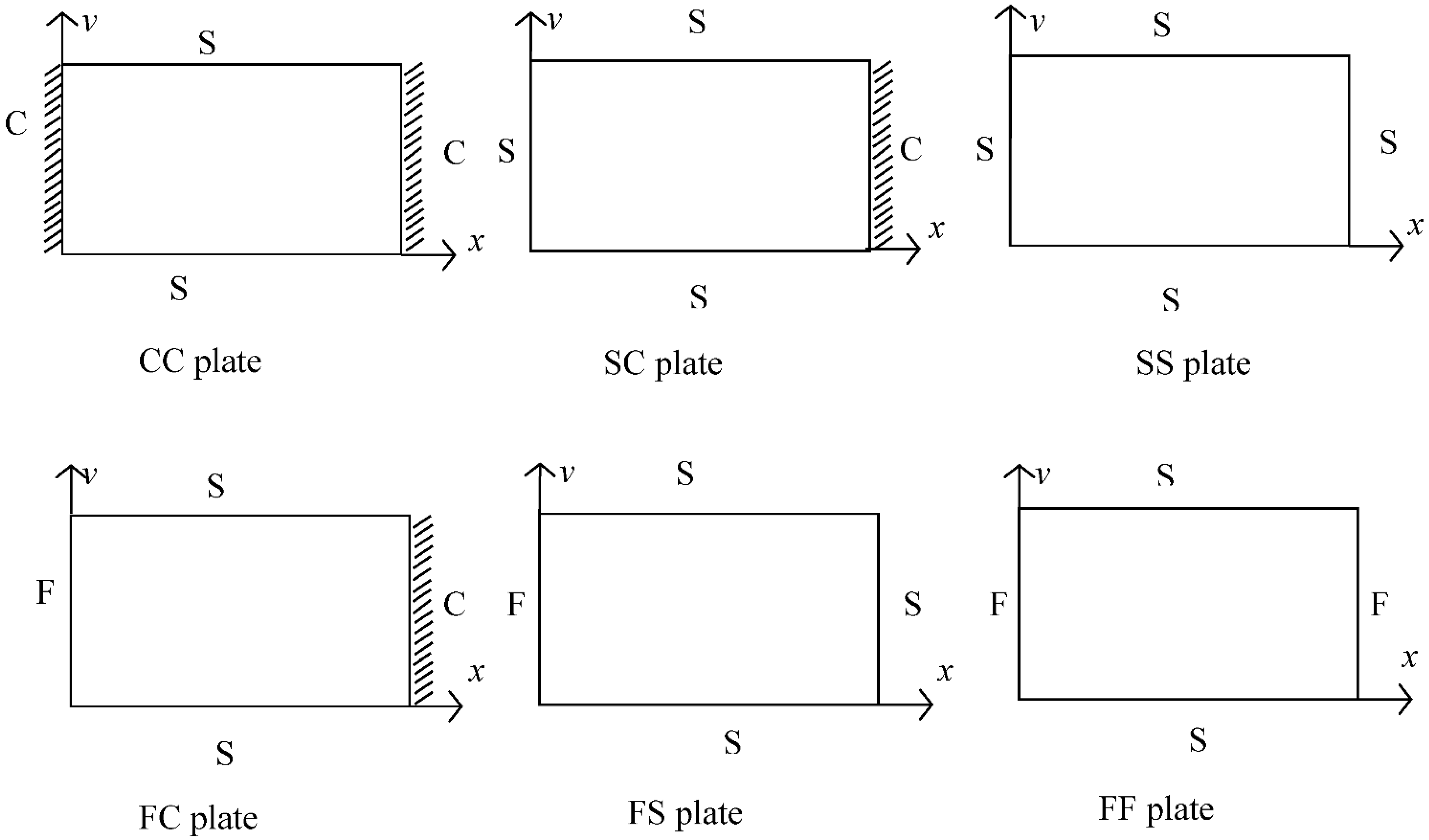
3.3. Boundary Conditions

The natural boundary conditions (BCs) are obtained by applying Hamilton’s principle, given by Equation (5).

$$\begin{gathered} V_x=D_x\frac{{\partial }^3{w}^0}{\partial x^3}+\left(\frac{D_{xy}}{2}-\frac{h^3}{6}{Q}_{66}\right)\frac{{\partial }^3{w}^0}{\partial x\partial y^2} \\ {M}_{xx}=D_x\frac{{\partial }^2{w}^0}{\partial x^2}-\frac{h^3}{12}{Q}_{12}\frac{{\partial }^2{w}^0}{\partial y^2} \end{gathered}$$

(5)

where $V_x$, $M_{xx}$ indicate the shear force and bending moments of the plate.

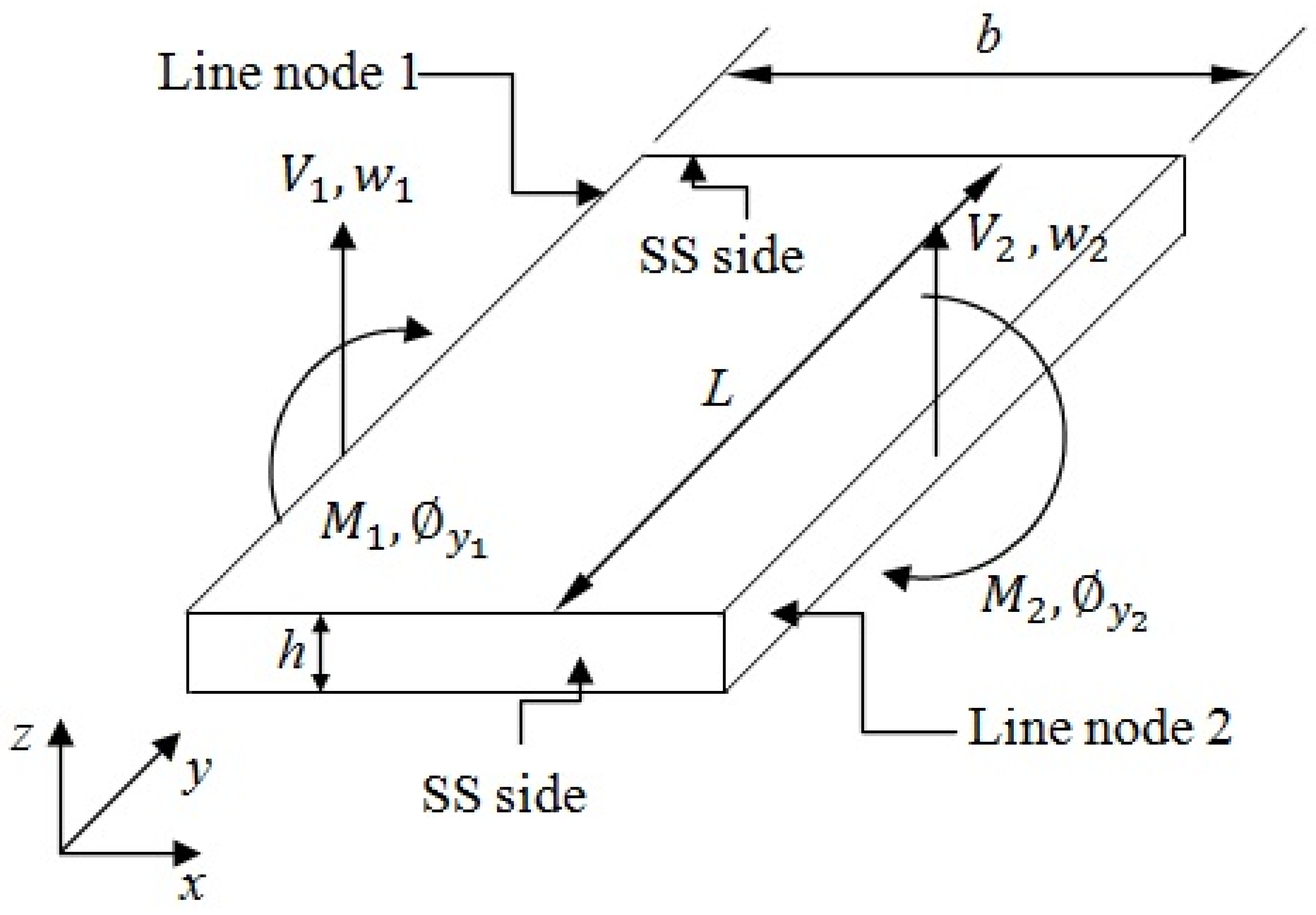
4. Formulation of Dynamic Stiffness (DS) Matrix with Levy Solution

The generalized differential Equation (3) is solved by applying force and displacement boundary conditions to develop the DS matrix. A Levy solution is implemented to solve Equation (3), and to satisfy the BCs given by Equation (5), it is sought in the given form as presented in Equation (6) [33].

$$w^0\left(x,y,t\right)={\displaystyle \sum }_{m=1}^{\infty }{w}_m\left(x\right)e^{i\omega t}\sin \left({\alpha }_{m}y\right) \mathrm{with} {\alpha }_m=\frac{m\pi }{L}\left(m=1,2,\dots \dots \dots \infty \right)$$

(6)

where $\omega$ represents the unknown frequency.

A generalized fourth-order ordinary differential equation is determined by substituting Equation (6) into Equation (3); it can be expressed as

$$D_x\frac{d^4{w}_m}{d{x}^4}-{\alpha }_m^2{D}_{xy}\frac{d^2{w}_m}{d{x}^2}+\left({\alpha }_m^4{D}_y+\rho h{\omega }^2\right)w_m=0$$

(7)

The developed Equation (7) produces the standard four roots; based on its nature, there are only two feasible solutions obtained and given by cases 1 and 2.

Case 1. ${\alpha }_m^2\ge \sqrt{{\alpha }_m^4\left(D_{xy}^2-4D_x{D}_y\right)-4D_x\rho h{\omega }^2}$

In the above case, all roots are real ($r_{1_m},-r_{1_m},r_{2_m},-r_{2_m}$) and can be expressed as

$$\begin{gathered} r_{1m}=\sqrt{\frac{{\alpha }_m^2{D}_{xy}+\sqrt{{\alpha }_m^4\left(D_{xy}^2-4D_x{D}_y\right)-4D_x\rho h{\omega }^2}}{2D_x}} \\ {r}_{2m}=\sqrt{\frac{{\alpha }_m^2{D}_{xy}-\sqrt{{\alpha }_m^4\left(D_{xy}^2-4D_x{D}_y\right)-4D_x\rho h{\omega }^2}}{2D_x}} \end{gathered}$$

$$\begin{gathered} r_{1m}=\sqrt{\frac{{\alpha }_m^2{D}_{xy}+\sqrt{{\alpha }_m^4\left(D_{xy}^2-4D_x{D}_y\right)-4D_x\rho h{\omega }^2}}{2D_x}} \\ r_{2m}=\sqrt{\frac{{\alpha }_m^2{D}_{xy}-\sqrt{{\alpha }_m^4\left(D_{xy}^2-4D_x{D}_y\right)-4D_x\rho h{\omega }^2}}{2D_x}} \end{gathered}$$

The solution is given by Equation (8).

$$w_m\left(x\right)=A_m\cos h\left(r_{1m}x\right)+B_m\sin h\left(r_{1m}x\right)+C_m\cos h\left(r_{2m}x\right)+D_m\sin h\left(r_{2m}x\right)$$

(8)

where $A_m, B_m, C_m, \mathrm{and} D_m$ are constants.

Case 2. ${\alpha }_m^2\le \sqrt{{\alpha }_m^4\left(D_{xy}^2-4D_x{D}_y\right)-4D_x\rho h{\omega }^2}$

In the above case are two real roots and two imaginary roots ($r_{1_m},-r_{1_m},i{r}_{2_m},-i{r}_{2_m}$), and can be expressed as

$$\begin{gathered} r_{1m}=\sqrt{\frac{{\alpha }_m^2{D}_{xy}+\sqrt{{\alpha }_m^4\left(D_{xy}^2-4D_x{D}_y\right)-4D_x\rho h{\omega }^2}}{2D_x}} \\ {r}_{2m}=\sqrt{\frac{-{\alpha }_m^2{D}_{xy}+\sqrt{{\alpha }_m^4\left(D_{xy}^2-4D_x{D}_y\right)-4D_x\rho h{\omega }^2}}{2D_x}} \end{gathered}$$

The solution is given by Equation (9).

$$w_m\left(x\right)=A_m\cos h\left(r_{1_m}x\right)+B_m\sin h\left(r_{1_m}x\right)+C_m\cos \left(r_{2_m}x\right)+A_m\cos \left(r_{2_m}x\right)$$

(9)

For case 1, the formulation of the DS matrix is explained below. A similar pattern is implemented for case 2, but is not explained here for brevity.

By applying Equations (6) and (8), the displacement $(w^0)$, bending rotation $({\varnothing }_y)$, shear force $\left(V_x\right)$, and moment $\left(M_{xx}\right)$ are determined and can be given by Equations (10)–(12).

$${\varphi }_{y_m}\left(x,y\right)={\varphi }_{y_m}\left(x\right)\sin \left({\alpha }_{m}y\right)$$

$$=\frac{-\partial w_m\left(x\right)}{\partial x}\sin \left({\alpha }_{m}y\right)$$

$$\begin{array}{c}\Rightarrow {\varphi }_{y_m}\left(x,y\right)=-[A_m{r}_{1m}\sin h\left(r_{1m}x\right)+B_m{r}_{1m}\cos h\left(r_{1m}x\right)+C_m{r}_{2m}\sin h\left(r_{2m}x\right)\\ +D_m{r}_{2m}\cos h\left(r_{2m}x\right)]\sin \left({\alpha }_{m}y\right)=\frac{-\partial w_m\left(x\right)}{\partial x}\sin \left({\alpha }_{m}y\right)\end{array}$$

(10)

$$\begin{gathered} V_{x_m}\left(x,y\right)=V_{x_m}\left(x\right)\sin \left({\alpha }_{m}y\right) \\ =\left[D_x\frac{{\partial }^3{w}^0}{\partial x^3}+\left(\frac{D_{xy}}{2}-\frac{h^3}{6}{Q}_{66}\right)\frac{{\partial }^3{w}^0}{\partial x\partial y^2}\right]\sin \left({\alpha }_{m}y\right) \end{gathered}$$

$$\begin{array}{c}\Rightarrow V_{x_m}\left(x,y\right)=[A_m\sin h\left(r_{1m}x\right)\left(D_x{r}_{1m}^3-H{r}_{1m}{\alpha }_m^2\right)+B_m\cos h\left(r_{1m}x\right)(D_x{r}_{1m}^3-H{r}_{1m}{\alpha }_m^2\\ +C_m\sin h\left(r_{2m}x\right)\left(D_x{r}_{2m}^3-H{r}_{2m}{\alpha }_m^2\right)\\ +D_m\cos h\left(r_{2m}x\right)\left(D_x{r}_{2m}^3-H{r}_{2m}{\alpha }_m^2\right)]\sin \left({\alpha }_{m}y\right)\end{array}$$

(11)

where $H=\left(\frac{D_{xy}}{2}-\frac{h^3}{6}{Q}_{66}\right)$.

$$\begin{gathered} M_{x{x}_m}\left(x,y\right)=M_{x{x}_m}\left(x\right)\sin \left({\alpha }_{m}y\right) \\ =\left(D_x\frac{{\partial }^2{w}^0}{\partial x^2}-\frac{h^3}{12}{Q}_{12}\frac{{\partial }^2{w}^0}{\partial y^2}\right)\sin \left({\alpha }_{m}y\right) \end{gathered}$$

$$\begin{gathered} \Rightarrow M_{x{x}_m}\left(x,y\right)=[A_m\cos h\left(r_{1m}x\right)\left(D_x{r}_{1_m}^2+I{\alpha }_m^2\right)+B_m\sin h\left(r_{1m}x\right)\left(D_x{r}_{1m}^2+I{\alpha }_m^2\right)+ \\ {C}_m\cos h\left(r_{2m}x\right)\left(D_x{r}_{2m}^2+I{\alpha }_m^2\right)+D_m\sin h\left(r_{2m}x\right)\left(D_x{r}_{2m}^2+I{\alpha }_m^2\right)]\sin \left({\alpha }_{m}y\right) \end{gathered}$$

(12)

where $I={{\displaystyle \int }}_{-h/2}^{h/2}\rho dz$.

The BCs for the Levy-type plate are represented in Figure 3.

The BCs for displacements are:

$$\begin{gathered} x=0, w_m=w_1; {\varnothing }_{ym}={\varnothing }_{y1} \\ x=b, w_m=w_2; {\varnothing }_{ym}={\varnothing }_{y2} \end{gathered}$$

(13)

The BCs for the forces are:

$$\begin{gathered} x=0, V_{xm}=-V_1; M_{xxm}=-M_1 \\ x=b, V_{xm}=V_2; M_{xxm}=M_2 \end{gathered}$$

(14)

The displacement BCs in Equation (13) are substituting into Equations (8) and (10); the following equations can be obtained as:

$$\begin{array}{l}{w}_1=A_m+0B_m+C_m+0D_m\\ {\varnothing }_{y1}=0A_m-r_{1m}{B}_m+0C_m-r_{2m}{D}_m\\ w_1=C{h}_1{A}_m+S{h}_1{B}_m+C{h}_2{C}_m+S{h}_2{D}_m\\ {\varnothing }_{y2}=\left(-r_{1m}S{h}_1\right)A_m-(r_{1m}C{h}_1)B_m-(r_{2m}S{h}_2)C_m-(r_{2m}C{h}_2)D_m\end{array}$$

where

$$\begin{array}{l}C{h}_1=\cos h(r_{1m}b), C{h}_2=\cos h(r_{2m}b)\\ S{h}_1=\sin h(r_{1m}b), S{h}_2=\sin h(r_{2m}b)\end{array}$$

This expression can be rewritten in the matrix form and expressed by Equation (15).

$$\left[\begin{array}{c}{w}_1\\ {\varnothing }_1\\ w_2\\ {\varnothing }_2\end{array}\right]=\left[\begin{array}{cccc}1& 0& 1& 0\\ 0& -r_{1m}& 0& r_{2m}\\ C{h}_1& S{h}_1& C{h}_2& S{h}_2\\ -r_{1m}S{h}_1& -r_{1m}C{h}_1& -r_{2m}S{h}_2& -r_{2m}C{h}_2\end{array}\right]\left\{\begin{array}{c}{A}_m\\ B_m\\ C_m\\ D_m\end{array}\right\}$$

(15)

i.e.,

$$\left[\delta \right]=\left[A\right]\left\{C\right\}$$

(16)

Similarly, the force BCs are applied; substituting Equation (14) into Equations (11) and (12), the following matrix relationship can be developed and expressed by Equation (17).

$$\left[\begin{array}{c}{V}_1\\ M_1\\ V_2\\ M_2\end{array}\right]=\left[\begin{array}{cccc}0& R_1& 0& R_2\\ L_1& 0& L_2& 0\\ -R_{1}S{h}_1& -R_{1}C{h}_1& -R_{2}S{h}_2& -R_{1}C{h}_2\\ -L_{1}C{h}_1& -L_{1}S{h}_1& -L_{2}C{h}_2& -L_{2}S{h}_2\end{array}\right]\left\{\begin{array}{c}{A}_m\\ B_m\\ C_m\\ D_m\end{array}\right\}.$$

(17)

i.e.,

$$\left[F\right]=\left[R\right]\left\{C\right\}$$

(18)

where

$$R_i=D_x{r}_{im}^3-H{r}_{im}{\alpha }_m^2, L_i=-D_x{r}_{im}^3-I{\alpha }_m^2$$

with i = 1,2.

By excluding the constant vector value of $C$, the following relationship can be formed as

$$\left[F\right]=\left[R\right]\left\{\delta \right\}$$

(19)

where

$$\left[K\right]=\left[R\right]{\left[A\right]}^{-1}$$

(20)

Thus, a square 4 × 4 symmetric DS matrix from Equation (20) is developed, including independent terms $(S_{vv}, S_{vm}, S_{mm}, F_{vv}, F_{vm}, F_{mm}$). Therefore, the generated DS matrix of the single plate element can be expressed as

$$\left[K\right]=\left[\begin{array}{cccc}{S}_{vv}& S_{vm}& F_{vv}& F_{vm}\\ S_{vm}& S_{mm}& -F_{vm}& F_{mm}\\ F_{vv}& -F_{vm}& S_{vv}& -S_{vm}\\ F_{vm}& F_{mm}& -S_{vm}& S_{mm}\end{array}\right]$$

(21)

The mathematical expressions of Equation (21) are explained in Appendix A.

4.1. Dynamic Stiffness (DS) Matrix Assembly Procedure with Boundary Conditions

The dynamic stiffness matrix given by Equation (21) was developed for a plate element. By obtaining the natural frequencies of a given orthotropic plate assembly, we considered four elements of the given plate geometry. Each element of the plate was connected through nodal lines. Since there were five nodal lines and the degree of freedom was two per element, a 10 × 10 global master stiffness matrix was formulated. The assembly procedure is similar to the finite element method, schematically shown in Figure 4. Boundary conditions can be applied the same way as we applied in the finite element method. The penalty method was applied as boundary conditions to suppress a particular degree of freedom. In this method, a considerable value of stiffness is added to the appropriate term on the leading diagonal of the dynamic stiffness matrix. The procedure for applying the boundary conditions is summarized as follows:

• Displacement $(W_i)$ is penalized for simply supported (S) boundary conditions.
• Displacement ($W_i)$ and rotation (${\varphi }_i)$ are penalized for clamped (C) boundary conditions.
• No penalty is implemented for the free (F) boundary condition.

where $i$ represents the suppressed node.

Figure 4. Assembly procedure of dynamic stiffness matrices.

Figure 4. Assembly procedure of dynamic stiffness matrices.

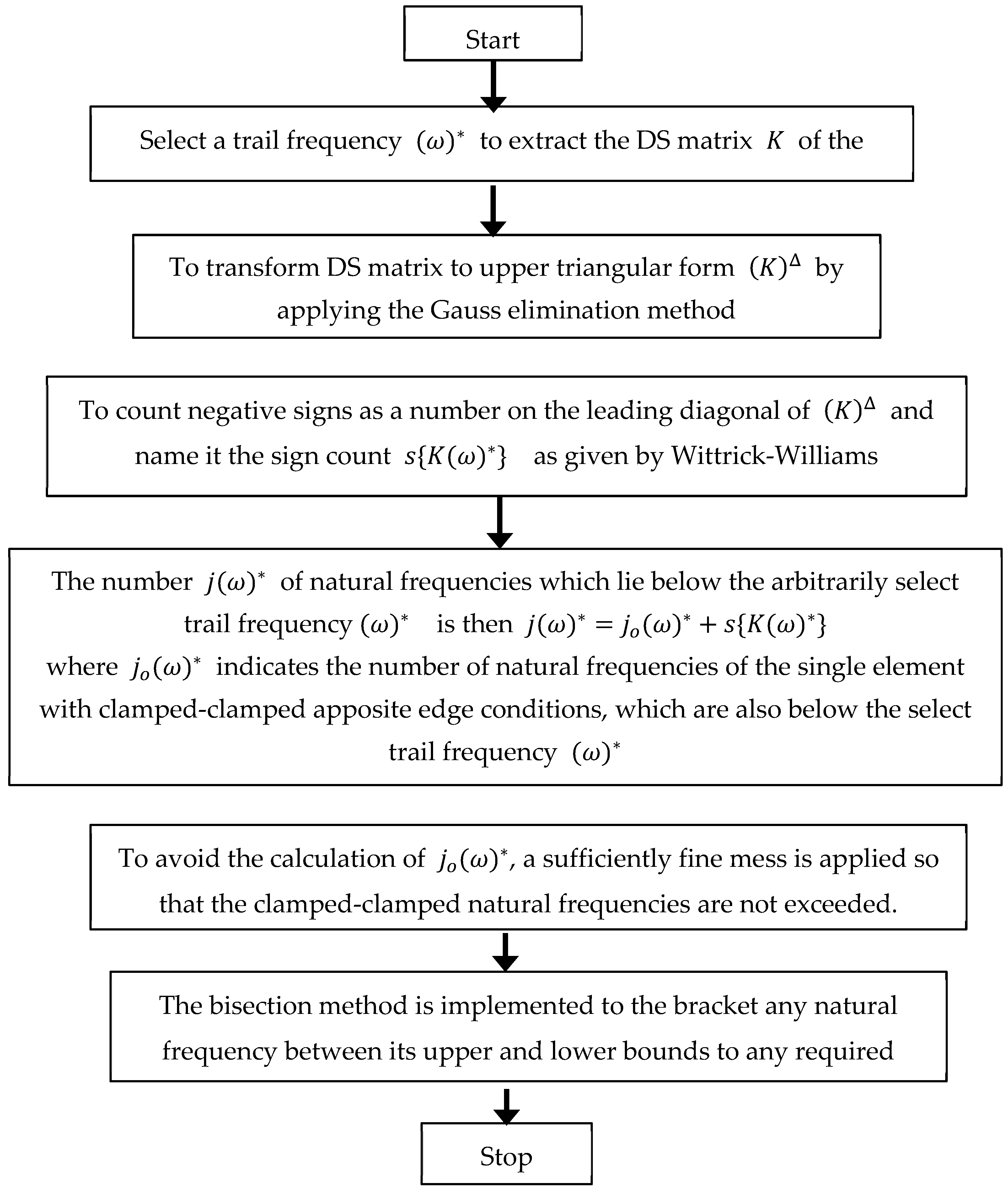
4.2. Application of the Wittrick and Williams (W–W) Algorithm

One way of determining the natural frequencies is by using the zeros of the global dynamic stiffness matrix of the structure under study. However, this method has its limitations due to the transcendental behavior of the DS elements, which makes the plot of the frequency determinant tedious. Moreover, sometimes this may lead to missing the coincident frequencies. So, to avoid these difficulties, the Wittrick–Williams algorithm [33,50] was used, which ensured that no natural frequencies were missed. The procedure to follow the W–W algorithm can be represented in a flow chart, shown in Figure 5.

5. Results and Discussions

This section presents the non-dimensional fundamental frequencies of an orthotropic rectangular plate with Levy-type BCs, i.e., two simply supported opposite edges and the other two edges having arbitrary boundary conditions. To simplify the problem, a two-letter notation was used to describe the boundary conditions of the remaining edges, as shown in Figure 2. For example, SC signifies that one edge is simply supported (S) and the other is clamped (C). The results obtained by DSM were compared with published results and the FEM using ANSYS. A detailed study and discussion were conducted to analyze the effects of the boundary conditions and the variations of the modulus ratio, aspect ratio, and thickness ratio on the fundamental natural frequency of an orthotropic plate. The following material properties were used for analysis [51]:

$$E_1/E_2 \mathrm{is} \mathrm{varied} \mathrm{from} 3 \mathrm{to} 50, G_{12}/E_2=G_{13}/E_2=0.5, G_{23}/E_2=0.2 {\vartheta }_{12}=0.25.$$

(22)

The non-dimensional fundamental natural frequency is calculated as [52]:

$$\varpi =\omega \frac{b^2}{h}\sqrt{\frac{\rho }{E_2}}$$

(23)

5.1. Comparative Study

A program in MATLAB was constructed to compute the fundamental natural frequencies of the plate. The natural frequencies obtained by DSM were compared against the results reported by Reddy and Phan [52] using CPT and with those reported by Thai and Kim [15] using the variable refined plate theory (RPT), as shown in

Table 1. Comparison of fundamental frequency parameters $\varpi =\omega \frac{b^2}{h}\sqrt{\frac{\rho }{E_2}}$ of the Levy-type orthotropic plate (b/h = 100).

b/L	E1/E2	Method	Boundary Conditions
			CC	SC	SS	FC	FS	FF
0.5	10	Ref [52]	20.6543	14.3450	9.3421	3.5614	1.3190	0.7124
		Ref [15]	20.5603	14.3137	9.3331	3.5600	1.3190	0.7123
		DSM	20.5857	14.3116	9.3209	3.5154	1.3188	0.7123
		FEM	20.6766	14.3565	9.3455	3.5558	1.3186	0.7141
		Error (%)	(−0.1234)	(0.0144)	(0.1309)	(1.2677)	(0.0152)	(0.0011)
	25	Ref [52]	32.4390	22.4259	14.4578	5.3051	1.3193	0.7123
		Ref [15]	32.0795	22.3069	14.4245	5.3003	1.3192	0.7122
		DSM	32.4229	22.4148	14.4507	5.3042	1.3191	0.7122
		FEM	32.2347	22.3539	14.4430	5.2925	1.3189	0.7141
		Error (%)	(−1.0590)	(−0.4813)	(−0.1815)	(−0.0735)	(0.0076)	(0.0000)
	40	Ref [52]	40.9633	28.2855	18.1876	6.6030	1.3194	0.7123
		Ref [15]	40.2478	28.0480	18.1215	6.5937	1.3193	0.7122
		DSM	40.9620	28.2846	18.1870	6.6010	1.3190	0.7122
		FEM	40.4100	28.0814	18.1426	6.5826	1.3189	0.7141
		Error (%)	(−1.7436)	(−0.8366)	(−0.3603)	(−0.1106)	(0.0227)	(0.0000)
1	10	Ref [52]	21.2889	15.2042	10.4963	5.0586	3.6114	2.8503
		Ref [15]	21.2078	15.1747	10.4863	5.0564	3.6105	2.8496
		DSM	21.2405	15.1709	10.4750	5.0144	3.6112	2.8501
		FEM	21.3090	15.2098	10.4949	5.0538	3.6125	2.8569
		Error (%)	(−0.1539)	(0.0248)	(0.1080)	(0.8376)	(−0.0194)	(−0.0175)
	25	Ref [52]	32.8464	22.9847	15.2278	6.4146	3.6118	2.8493
		Ref [15]	32.5515	22.8835	15.1972	6.4100	3.6110	2.8486
		DSM	32.8303	22.9736	15.2207	6.4014	3.6115	2.8490
		FEM	32.6351	22.9073	15.2089	6.4025	3.6128	2.8558
		Error (%)	(−0.8491)	(−0.3921)	(−0.1544)	(0.1343)	(−0.0138)	(−0.0140)
	40	Ref [52]	41.2866	28.7305	18.8052	7.5253	3.6121	2.8492
		Ref [15]	40.7062	28.5337	18.7477	7.5178	3.6112	2.8485
		DSM	41.2853	28.7296	18.8046	7.5045	3.6120	2.8491
		FEM	40.7277	28.5213	18.7566	7.5051	3.6130	2.8557
		Error (%)	(−1.4027)	(−0.6818)	(−0.3028)	(0.1772)	(−0.0221)	(−0.0211)
2	10	Ref [52]	25.5184	20.5941	17.1364	12.9377	12.2379	11.4094
		Ref [15]	25.4427	20.5543	17.1129	12.9238	12.2259	11.3981
		DSM	25.4651	20.5536	17.1046	12.9145	12.2298	11.3998
		FEM	25.4958	20.5658	17.1086	12.9324	12.2395	11.4254
		Error (%)	(−0.0879)	(0.0032)	(0.0483)	(0.0720)	(−0.0319)	(−0.0149)
	25	Ref [52]	35.7303	26.8537	20.3682	13.5562	12.2305	11.3993
		Ref [15]	35.5237	26.7659	20.3288	13.5404	12.2186	11.3880
		DSM	35.7135	26.8417	20.3596	13.5504	12.2301	11.3895
		FEM	35.4925	26.7502	20.3265	13.5433	12.2319	11.4155
		Error (%)	(−0.5316)	(−0.2822)	(−0.1514)	(−0.0738)	(−0.0940)	(−0.0132)
	40	Ref [52]	43.6154	31.9099	23.1622	14.1271	12.2301	11.3977
		Ref [15]	43.2415	31.7630	23.1043	14.1093	12.2182	11.3864
		DSM	43.6141	31.9090	23.1616	14.1270	12.2298	11.3944
		FEM	43.0347	31.6809	23.0942	14.1072	12.2312	11.4140
		Error (%)	(−0.8543)	(−0.4576)	(−0.2473)	(−0.1253)	(−0.0949)	(−0.0702)

; errors incurred by DSM when compared with Ref. [15] are reported in the brackets. The natural frequency changes for different boundary conditions (due to a change in stiffness) were noticed in Table 1. The maximum value of natural frequencies is reported for the CC boundary condition; the minimum value was obtained for the FF boundary condition. In the CC boundary condition, more constraints were introduced at the edges of the plate, which increased the stiffness of the plate, resulting in a higher natural frequency. On the other hand, in the FF boundary condition, no constraint was applied at the edges of the plate, which decreased the stiffness of the plate, and lowered the natural frequency, as shown in Table 1.

It is observed from Table 1 that the maximum error is −1.7436% for the CC boundary condition at b/L = 0.5 and E₁/E₂ = 40, whereas the minimum error encountered is 0.00% at b/L = 0.5 and E₁/E₂ = 25 for the FF boundary condition. It can be seen from Table 1 that most of the errors lie within 2%. It is observed that the DSM results of a thin orthotropic plate in Table 1 are in excellent agreement with the published literature and the FEM results.

5.2. Parameter Studies

To study the effects of different boundary conditions, variations of thickness ratio, modulus ratio, and aspect ratio on the non-dimensional fundamental frequencies of thin orthotropic plates, parametric studies were conducted. The DSM results are also compared with the FEM obtained by ANSYS. For the modeling of the plate, shell element 181 was used in ANSYS. To test the accuracy of FEM, the non-dimensional fundamental frequencies were obtained by DSM based on CPT for a simply supported Levy-type orthotropic plate (b/L = 1, b/h = 20) at different modulus ratios, compared to the values obtained by FEM with different mesh sizes, as shown in

Table 2. Obtained results for the test accuracy of the finite element mesh.

	E1/E2
	3	10	20	30	40	50
DSM	7.1504	10.2475	13.4417	15.7097	17.4294	19.0676
20 × 20 FEM	7.0938	10.1434	13.1326	15.3657	17.1616	18.6632
40 × 40 FEM	7.0610	10.1132	13.1070	15.3336	17.1285	18.6298
80 × 80 FEM	7.0507	10.1040	13.0932	15.3250	17.1192	18.6203
100 × 100 FEM	7.0494	10.1030	13.0918	15.3239	17.1179	18.6188

. A very good convergence between the FEM and DSM results can be observed. The final choice is a mesh with 20 × 20 plate elements, which is a good compromise between the need for accuracy and limiting the computing time. In

Table 3. Comparison of the fundamental frequency parameters $\left(\varpi =\omega \frac{b^2}{h}\sqrt{\frac{\rho }{E_2}}\right)$ of the orthotropic plate with the SC boundary conditions.

b/L	b/h	Method	E1/E2
			3	10	20	30	40	50
0.5	20	RPT [15]	8.0410	13.6063	18.2286	21.3634	23.7191	25.5851
		DTM [53]	8.0500	-	18.2250	21.3750	23.7500	25.7900
		TCM [53]	8.0418	-	18.2310	21.3647	23.7211	25.5865
		DSM	8.0368	13.5844	18.1881	21.3584	23.7235	25.2657
		FEM	8.0196	13.4668	17.8312	20.6852	21.7298	21.7850
		Error (%)	0.0523	0.1609	0.2227	0.0234	−0.0184	1.2642
	50	RPT 15]	8.1690	14.2179	19.7562	23.9265	27.3668	30.3311
		DTM [53]	8.1750	-	19.9270	23.9440	27.4445	30.4350
		TCM [53]	8.1692	-	19.7581	23.9296	27.3706	30.3356
		DSM	8.1648	14.2078	19.7124	23.9210	27.3718	30.3117
		FEM	8.1883	14.2348	19.7344	23.8543	27.2119	30.0908
		Error (%)	0.0514	0.0711	0.2222	0.0232	−0.0184	0.0639
1	20	RPT [15]	9.4219	14.2277	19.0510	22.2738	24.7632	26.7775
		DTM [53]	9.3740	-	19.1240	22.3250	24.8120	26.9144
		TCM [53]	9.4227	-	18.3073	22.2747	24.7638	26.7789
		DSM	9.4305	14.2204	19.3911	22.2704	24.7508	26.6002
		FEM	9.3187	15.0824	18.3699	21.0717	23.2367	25.3476
		Error (%)	−0.0912	0.0513	−1.7539	0.0153	0.0501	0.6665
	50	RPT [15]	9.5898	14.4921	20.4197	24.5288	27.9597	30.9416
		DTM [53]	9.4265	-	20.5705	24.5450	27.9880	30.8850
		TCM [53]	9.5900	-	20.4210	24.5305	27.9616	30.9441
		DSM	9.5986	14.5044	20.4134	24.5251	27.9457	30.7368
		FEM	9.5888	15.0722	20.3359	24.3373	27.6373	30.4720
		Error (%)	−0.0919	−0.0848	0.0310	0.0149	0.0500	0.6664
2	20	RPT [15]	16.3187	19.5797	23.2516	26.1972	28.6627	30.7812
		DTM [53]	16.3940	-	23.3000	26.2455	28.7151	30.8502
		TCM [53]	16.3198	-	23.2521	26.1978	28.6630	30.7814
		DSM	16.3173	19.5944	23.2510	26.1632	28.6581	30.7657
		FEM	16.2784	19.5250	23.1165	26.7783	28.1530	30.4003
	50	Error (%)	0.0086	−0.0750	0.0026	0.1300	0.0161	0.0504
		RPT [15]	16.8218	20.4196	24.6437	28.1975	31.3099	34.1026
		DTM [53]	16.8825	-	24.6202	28.2062	31.3150	34.1000
		TCM [53]	16.8221	-	24.6442	28.1982	31.3105	34.1033
		DSM	16.8204	20.4214	24.6431	28.1609	31.3050	34.0855
		FEM	16.7497	20.339	24.462	27.8501	30.7535	33.3047
		Error (%)	0.0084	−0.0088	0.0024	0.1298	0.0158	0.0502

,

Table 4. Comparison of the fundamental frequency parameters $\left(\varpi =\omega \frac{b^2}{h}\sqrt{\frac{\rho }{E_2}}\right)$ of the orthotropic plate with the SS boundary conditions.

b/L	b/h	Method	E1/E2
			3	10	20	30	40	50
0.5	20	RPT [15]	5.4685	9.1141	12.4009	14.7974	16.7105	18.3073
		DTM [53]	5.4774	-	12.4005	14.7975	16.7100	18.3070
		TCM [53]	5.4685	-	12.4009	14.7974	16.7105	18.3073
		DSM	5.4996	9.1045	12.4112	14.9467	16.6942	18.3017
		FEM	5.4419	9.0998	12.3710	14.7391	16.6188	18.1777
		Error (%)	−0.5655	0.1054	−0.0830	−0.9989	0.0976	0.0306
	50	RPT [15]	5.5126	9.3044	12.8804	15.6246	17.9239	19.9333
		DTM [53]	5.5000	-	12.9060	15.6250	17.9240	19.9300
		TCM [53]	5.5126	-	12.8804	15.6247	17.9239	19.9333
		DSM	5.4609	9.3130	12.9564	15.7823	17.9064	19.9273
		FEM	5.5125	9.3014	12.8910	15.5475	17.9278	19.9310
		Error (%)	0.9476	−0.0923	−0.5867	−0.9992	0.0975	0.0301
1	20	RPT [15]	7.2194	10.2349	13.2676	15.5845	17.4839	19.1002
		DTM [53]	7.2200	-	13.2500	15.5840	17.4835	19.1000
		TCM [53]	7.2194	-	13.2676	15.5846	17.4839	19.1002
		DSM	7.1504	10.2475	13.4417	15.7097	17.4294	19.0676
		FEM	7.0938	10.1434	13.1326	15.3657	17.1616	18.6632
		Error (%)	0.9650	−0.1230	−1.2952	−0.7970	0.3127	0.1710
	50	RPT [15]	7.3012	10.4530	13.7360	16.3474	18.5726	20.5377
		DTM [53]	7.3000	-	13.7600	16.3772	18.6072	20.5765
		TCM [53]	7.3012	-	13.7360	16.3474	18.5726	20.5377
		DSM	7.2312	10.4555	13.7963	16.4788	18.5149	20.5027
		FEM	7.2778	10.4426	13.7230	16.3228	18.5285	20.4713
		Error (%)	0.9686	−0.0239	−0.4370	−0.7972	0.3119	0.1705
2	20	RPT [15]	14.9772	16.5030	18.4742	20.2036	21.7468	23.1427
		DTM [53]	14.9795	-	18.4740	20.2036	21.7469	23.1428
		TCM [53]	14.9773	-	18.4742	20.2036	21.7468	23.1427
		DSM	14.7602	16.5247	18.5482	20.3326	21.6428	23.0351
		FEM	14.6185	16.2143	18.1645	19.7863	21.1685	22.3638
		Error (%)	1.4702	−0.1313	−0.3990	−0.6344	0.4805	0.4671
	50	RPT [15]	15.3796	17.0294	19.1992	21.1436	22.9151	24.5504
		DTM [53]	15.3502	-	19.2156	21.1663	22.9120	24.5480
		TCM [53]	15.3796	-	19.1992	21.1436	22.9151	24.5504
		DSM	15.2813	17.0145	19.2761	21.2786	22.8056	24.4363
		FEM	15.2894	16.9572	19.1294	21.0565	22.7983	24.3920
		Error (%)	0.6430	0.0876	−0.3989	−0.6347	0.4803	0.4670

,

Table 5. Comparison of the fundamental frequency parameters $\left(\varpi =\omega \frac{b^2}{h}\sqrt{\frac{\rho }{E_2}}\right)$ of the orthotropic plate with the SF boundary conditions.

b/L	b/h	Method	E1/E2
			3	10	20	30	40	50
0.5	20	RPT [15]	1.3160	1.3163	1.3165	1.3166	1.3166	1.3167
		DTM [53]	1.3164	-	1.3165	1.3166	1.3168	1.3169
		TCM [53]	1.3161	-	1.3165	1.3166	1.3167	1.3167
		DSM	1.3162	1.3162	1.3162	1.3164	1.3164	1.3165
		FEM	1.2903	1.2903	1.2906	1.2906	1.2906	1.2906
		Error (%)	−0.0152	0.0076	0.0228	0.0152	0.0152	0.0152
	50	RPT [15]	1.3183	1.3186	1.3188	1.3189	1.3189	1.3189
		DTM [53]	1.3189	-	1.3189	1.3190	1.3190	1.3190
		TCM [53]	1.3183	-	1.3188	1.3189	1.3189	1.3190
		DSM	1.3118	1.3154	1.3187	1.3187	1.3870	1.3880
		FEM	1.3133	1.3135	1.3137	1.3138	1.3137	1.3138
		Error (%)	0.4946	0.2433	0.0076	0.0152	0.0152	0.0076
1	20	RPT [15]	3.5900	3.5851	3.5854	3.5857	3.5858	3.5859
		DTM [53]	3.5949	-	3.5875	3.5874	3.5876	3.5877
		TCM [53]	3.5900	-	3.5855	3.5857	3.5859	3.5860
		DSM	3.5949	3.5901	3.5853	3.5856	3.5857	3.5885
		FEM	3.5358	3.5303	3.5300	3.5301	3.5301	3.5302
		Error (%)	−0.1363	−0.1393	0.0028	0.0028	0.0028	−0.0725
	50	RPT [15]	3.6121	3.6072	3.6074	3.6077	3.6079	3.6080
		DTM [53]	3.6309	-	3.6080	3.6082	3.6084	3.6085
		TCM [53]	3.6122	-	3.6075	3.6078	3.6080	3.6081
		DSM	3.6108	3.6001	3.6001	3.6066	3.6078	3.6079
		FEM	3.6039	3.5986	3.5984	3.5991	3.5991	3.5991
		Error (%)	0.0371	0.1972	0.2028	0.0305	0.0028	0.0028
2	20	RPT [15]	11.9528	11.9012	11.8952	11.8945	11.8944	11.8946
		DTM [53]	12.0400	-	11.9100	11.9000	11.9000	11.9050
		TCM [53]	11.9551	-	11.8960	11.8949	11.8947	11.8947
		DSM	11.9520	11.8951	11.8950	11.8948	11.8946	11.8946
		FEM	11.8526	11.8090	11.7943	11.7919	11.7910	11.7906
		Error (%)	0.0067	0.0513	0.0017	−0.0025	−0.0017	0.0000
	50	RPT [15]	12.2370	12.1817	12.1752	12.1743	12.1742	12.1742
		DTM [53]	12.3926	-	12.1802	12.1792	12.1790	12.1791
		TCM [53]	12.2375	-	12.1755	12.1745	12.1744	12.1745
		DSM	12.2370	12.1785	12.1751	12.1744	12.1742	12.1742
		FEM	12.2274	12.1720	12.1655	12.1655	12.1632	12.1631
		Error (%)	0.0000	0.0263	0.0008	−0.0008	0.0000	0.0000

,

Table 6. Comparison of the fundamental frequency parameters $\left(\varpi =\omega \frac{b^2}{h}\sqrt{\frac{\rho }{E_2}}\right)$ of an orthotropic plate with the CC boundary conditions.

b/L	b/h	Method	E1/E2
			3	10	20	30	40	50
0.5	20	RPT [15]	11.1940	18.6410	24.1770	27.5890	29.9780	31.7720
		DTM [53]	-	-	-	-	-	-
		TCM [53]	-	-	-	-	-	-
		DSM	11.0440	18.5440	24.0010	27.4220	29.8140	31.6450
		FEM	11.2241	18.5395	23.7936	26.9128	29.0241	30.5589
		Error (%)	1.3582	0.5231	0.7333	0.6090	0.5501	0.4013
	50	RPT [15]	11.5350	20.2830	28.0500	33.7400	38.3200	42.1780
		DTM [53]	-	-	-	-	-	-
		TCM [53]	-	-	-	-	-	-
		DSM	11.4450	20.0450	28.0010	33.4520	38.0150	42.0040
		FEM	11.5988	20.3688	28.1096	33.7420	38.2453	42.0120
		Error (%)	0.7864	1.1873	0.1750	0.8609	0.8023	0.4142
1	20	RPT [15]	12.2680	19.4910	25.2600	28.9750	31.6500	33.6990
		DTM [53]	-	-	-	-	-	-
		TCM [53]	-	-	-	-	-	-
		DSM	12.0540	19.3540	25.2600	28.8990	31.6498	33.6880
		FEM	12.2199	19.0866	24.1686	27.2132	29.2816	30.7884
		Error (%)	1.7720	0.7079	0.0000	0.2630	0.0006	0.0327
	50	RPT [15]	12.6300	20.9640	28.6650	34.4150	39.1030	43.0940
		DTM [53]	-	-	-	-	-	-
		TCM [53]	-	-	-	-	-	-
		DSM	12.6300	20.9620	28.6420	34.3440	39.0050	43.0920
		FEM	12.6752	20.9800	28.5476	34.0931	38.5449	42.2785
		Error (%)	0.0000	0.0095	0.0803	0.2067	0.2512	0.0046
2	20	RPT [15]	18.1620	23.7190	29.2240	33.2480	36.3950	38.9550
		DTM [53]	-	-	-	-	-	-
		TCM [53]	-	-	-	-	-	-
		DSM	18.0450	23.7180	29.2140	33.1450	36.3470	38.5450
		FEM	17.9076	22.9240	27.1301	29.7723	31.6051	32.9569
		Error (%)	0.6484	0.0042	0.0342	0.3108	0.1321	1.0637
	50	RPT [15]	18.8420	25.1990	32.0380	37.5070	42.1470	46.2150
		DTM [53]	-	-	-	-	-	-
		TCM [53]	-	-	-	-	-	-
		DSM	18.7540	24.9880	31.8970	37.1240	41.8740	46.0240
		FEM	18.8150	25.1027	31.6413	36.6844	40.8220	44.3360
		Error (%)	0.4692	0.8444	0.4420	1.0317	0.6520	0.4150

,

Table 7. Comparison of the fundamental frequency parameters $\left(\varpi =\omega \frac{b^2}{h}\sqrt{\frac{\rho }{E_2}}\right)$ of an orthotropic plate with the FC boundary conditions.

b/L	b/h	Method	E1/E2
			3	10	20	30	40	50
0.5	20	RPT [15]	2.3220	3.5230	4.7060	5.6190	6.3810	7.0410
		DTM [53]	-	-	-	-	-	-
		TCM [53]	-	-	-	-	-	-
		DSM	2.3210	3.5220	4.6990	5.6180	6.3740	7.0010
		FEM	2.3013	3.4995	4.6668	4.5382	6.2941	6.9261
		Error (%)	0.0431	0.0284	0.1490	0.0178	0.1098	0.5713
	50	RPT [15]	2.3320	3.5550	4.7800	5.7450	6.5660	7.2910
		DTM [53]	-	-	-	-	-	-
		TCM [53]	-	-	-	-	-	-
		DSM	2.3310	3.5350	4.7010	5.7440	6.5540	7.2870
		FEM	2.3266	3.5479	4.7691	4.6778	6.5441	7.2632
		Error (%)	0.0429	0.5658	1.6805	0.0174	0.1831	0.0549
1	20	RPT [15]	4.2160	4.9950	5.8970	6.6620	7.3360	7.9420
		DTM [53]	-	-	-	-	-	-
		TCM [53]	-	-	-	-	-	-
		DSM	4.2160	4.9920	5.8240	6.5770	7.2540	7.8450
		FEM	4.1595	4.9287	5.8066	6.5343	7.1612	7.7141
		Error (%)	0.0000	0.0601	1.2534	1.2924	1.1304	1.2365
	50	RPT [15]	4.2500	5.0480	5.9820	6.7820	7.4940	8.1420
		DTM [53]	-	-	-	-	-	-
		TCM [53]	-	-	-	-	-	-
		DSM	4.2450	5.0120	5.8440	6.4510	7.4240	8.0140
		FEM	4.2402	5.0346	5.9620	6.7541	7.4569	8.0942
		Error (%)	0.1178	0.7183	2.3614	5.1310	0.9429	1.5972
2	20	RPT [15]	12.2640	12.5540	12.9420	13.3020	13.6470	13.9780
		DTM [53]	-	-	-	-	-	-
		TCM [53]	-	-	-	-	-	-
		DSM	12.1240	12.4510	12.8450	13.2040	13.6140	13.8540
		FEM	11.8526	12.4252	12.7885	13.1213	13.4293	13.7178
		Error (%)	1.1547	0.8272	0.7552	0.7422	0.2424	0.8950
	50	RPT [15]	12.5670	12.8740	13.2880	13.6750	14.0460	14.4050
		DTM [53]	-	-	-	-	-	-
		TCM [53]	-	-	-	-	-	-
		DSM	12.4570	12.7450	13.1440	13.2470	14.0440	14.4020
		FEM	12.2274	12.5838	13.2596	13.6953	14.0022	14.3510
		Error (%)	0.8830	1.0122	1.0956	3.2309	0.0142	0.0208

and

Table 8. Comparison of the fundamental frequency parameters $\left(\varpi =\omega \frac{b^2}{h}\sqrt{\frac{\rho }{E_2}}\right)$ of an orthotropic plate with the FF boundary conditions.

b/L	b/h	Method	E1/E2
			3	10	20	30	40	50
0.5	20	RPT [15]	2.3250	2.3260	2.3260	2.3260	2.3260	2.3260
		DTM [53]	-	-	-	-	-	-
		TCM [53]	-	-	-	-	-	-
		DSM	2.3240	2.3250	2.3258	2.3258	2.3258	2.3258
		FEM	2.3252	2.3245	2.3260	2.3266	2.3260	2.3260
		Error (%)	0.0430	0.0430	0.0086	0.0086	0.0086	0.0086
	50	RPT [15]	2.3310	2.3310	2.3320	2.3320	2.3320	2.3320
		DTM [53]	-	-	-	-	-	-
		TCM [53]	-	-	-	-	-	-
		DSM	2.3312	2.335	2.3322	2.3325	2.3328	2.3320
		FEM	2.3315	2.3315	2.3325	2.3325	2.3325	2.3325
		Error (%)	−0.0086	−0.1716	−0.0086	−0.0214	−0.0343	0.0000
1	20	RPT [15]	2.8380	2.8300	2.8290	2.8290	2.8290	2.8290
		DTM [53]	-	-	-	-	-	-
		TCM [53]	-	-	-	-	-	-
		DSM	2.8140	2.8244	2.8344	2.8344	2.8344	2.8344
		FEM	2.8440	2.8371	2.8364	2.8466	2.8466	2.8466
		Error (%)	0.8529	0.1983	−0.1905	−0.1905	−0.1905	−0.1905
	50	RPT [15]	2.8560	2.8470	2.8460	2.8460	2.8460	2.8460
		DTM [53]	-	-	-	-	-	-
		TCM [53]	-	-	-	-	-	-
		DSM	2.8488	2.8444	2.8442	2.8442	2.8442	2.8442
		FEM	2.8626	2.8543	2.8534	2.8549	2.8549	2.8549
		Error (%)	0.2527	0.0914	0.0633	0.0633	0.0633	0.0633
2	20	RPT [15]	11.1510	11.0960	11.0880	11.0860	11.0850	11.0850
		DTM [53]	-	-	-	-	-	-
		TCM [53]	-	-	-	-	-	-
		DSM	11.1500	11.0900	11.0820	11.0810	11.0810	11.0810
		FEM	11.3046	11.1211	11.2471	11.2455	11.2455	11.2455
		Error (%)	0.0090	0.0541	0.0541	0.0451	0.0361	0.0361
	50	RPT [15]	11.4160	11.3570	11.3490	11.3460	11.3460	11.3450
		DTM [53]	-	-	-	-	-	-
		TCM [53]	-	-	-	-	-	-
		DSM	11.3967	11.3450	11.3460	11.3460	11.3450	11.3450
		FEM	11.4429	11.3850	11.3778	11.3759	11.3759	11.3759
		Error (%)	0.1695	0.1058	0.0264	0.0000	0.0088	0.0000

, the DSM results are compared against the published results reported by Mukhtar [53] using the differential transform method (DTM) and Taylor collocation method (TCM), and with those reported by authors [15] for different Young’s modulus ratios (E₁/E₂), aspect ratios (b/L), and thickness ratios (b/h). It could be observed from Table 3, Table 4, Table 5, Table 6, Table 7 and Table 8 that the natural frequencies, in general, decrease with an increase in Young’s modulus, aspect ratio, and thickness ratio for the orthotropic plate. It is observed in Table 3, Table 4, Table 5, Table 6 and Table 7 that with boundary conditions changing from SC to SF, the natural frequencies increase, with the increase in the modulus ratio (E₁/E₂) from 3 to 50 because of an increase in the stiffness of the plate. Compared with Ref. [15], the relative errors of DSM are reported in brackets in Table 3, Table 4, Table 5, Table 6, Table 7 and Table 8.

It could be observed from Table 3, Table 4, Table 5, Table 6, Table 7 and Table 8 that the maximum errors encountered in the DSM results when compared with Ref. [15] results are 1.7720% at b/L = 1.0, b/h = 20, and E₁/E₂ = 3 for the CC plate in Table 6. The next highest percentage of errors is −1.7539 (for the SC plate at b/L = 1, b/h = 20 and E₁/E₂ = 20) in Table 8. Thus, for all cases reported in Table 3, Table 4, Table 5, Table 6, Table 7 and Table 8, the error is less than 2%.

The effect of Young’s modulus ratio (E₁/E₂) and the thickness ratio (a/h) on natural frequencies for all boundary conditions are presented in Figure 6 and Figure 7, respectively. The following observations are obtained from Figure 6 and Figure 7, respectively.

(a) The natural frequency increases with increases in the modulus ratio $\left(\frac{E_1}{E_2}\right)$ for a given value of the side-thickness ratio (b/L = 0.5), as shown in Figure 6 for all boundary conditions, except FF and FS boundary conditions. The natural frequency values are nearly constant for FF and FS boundary conditions.

(b) The fundamental natural frequency values increase with increases in the side to thickness ratio (b/h) for a given Young’s modulus ratio $\left(\frac{E_1}{E_2}\right)$, as shown in Figure 7 for all boundary conditions except FF and FS boundaries.

6. Conclusions

In the present paper, the dynamic stiffness method, as a novel method, was implemented to analyze the out-of-plane free vibration of the rectangular orthotropic plate, where two opposite edges are simply supported. The classical plate theory was used to formulate the dynamic stiffness matrix for the rectangular orthotropic plate. The Wittrick–Williams algorithm was applied to solve the transcendental nature of the global dynamic stiffness matrix to extract the natural frequencies of the overall plate. The complete procedure, starting from developing the dynamic stiffness matrix and calculating natural frequencies, was implemented in a computer program using MATLAB. This enabled computation of any number of exact natural frequencies of the orthotropic plate for the Levy-type boundary conditions. The computed natural frequencies were compared against published results obtained by the finite element method using commercial software ANSYS. A new dataset on the natural frequencies for different aspect ratios, modulus ratios, and thickness ratios was computed and compared with the published literature.

The new results on natural frequency obtained by the DSM method can be implemented as a benchmark solution for future comparison purposes.

References

- Rayleigh, L. The Theory of Sound; Macmillan: Dover, NY, USA, 1945; Volume I, pp. 35–42. [Google Scholar]
- Ritz, W. On a new method for solving certain variational problems in mathematical physics. Crelle’s J. 1909, 1–61. [Google Scholar] [CrossRef]
- Bhat, R.B. Natural frequencies of rectangular plates using characteristic orthogonal polynomials in the Rayleigh-Ritz method. J. Sound Vib. 1985, 102, 493–499. [Google Scholar] [CrossRef]
- Gorman, D.J. Accurate free vibration analysis of the completely free orthotropic rectangular plate by the superposition method. J. Sound Vib. 1993, 165, 409–420. [Google Scholar] [CrossRef]
- Kshirsagar, S.; Bhaskar, K. Accurate and elegant free vibration and buckling studies of orthotropic rectangular plates using untruncated infinite series. J. Sound Vib. 2008, 314, 837–850. [Google Scholar] [CrossRef]
- Dalaei, M.; Kerr, A.D. Natural vibration analysis of clamped rectangular orthotropic plates. J. Sound Vib. 1996, 189, 399–406. [Google Scholar] [CrossRef]
- Bercin, A.N. Free vibration solution for clamped orthotropic plates using the Kantorovich method. J. Sound Vib. 1996, 196, 243–247. [Google Scholar] [CrossRef]
- Sakata, T.; Takahashi, K.; Bhat, R.B. Natural frequencies of orthotropic rectangular plates obtained by iterative reduction of the partial differential equation. J. Sound Vib. 1996, 189, 89–101. [Google Scholar] [CrossRef]
- Yu, S.D.; Cleghorn, W.L. Generic free vibration of orthotropic rectangular plates with clamped and simply supported edges. J. Sound Vib. 1993, 163, 439–450. [Google Scholar] [CrossRef]
- Timoshenko, S.; Woinowsky-Krieger, S. Theory of Plates and Shells; McGraw-Hill: New York, NY, USA, 1959. [Google Scholar]
- Leissa, A.W. Free vibration of rectangular plates. J. Sound Vib. 1973, 31, 257–293. [Google Scholar] [CrossRef]
- Gorman, D.J. Free Vibration Analysis of Rectangular Plates; Elsevier: Amsterdam, The Netherlands, 1982. [Google Scholar]
- Gorman, D.J. Accurate free vibration analysis of clamped orthotropic plates by the method of superposition. J. Sound Vib. 1990, 140, 391–411. [Google Scholar] [CrossRef]
- Biancolini, M.E.; Brutti, C.; Reccia, L. Approximate solution for free vibrations of thin orthotropic rectangular plates. J. Sound Vib. 2005, 288, 321–344. [Google Scholar] [CrossRef]
- Thai, H.; Kim, S.E. Levy-type solution for free vibration analysis of orthotropic plates based on two variable refined plate theory. Appl. Math. Model. 2012, 36, 3870–3882. [Google Scholar] [CrossRef]
- Xing, Y.F.; Liu, B. New exact solutions for free vibrations of thin orthotropic rectangular plates. Compos. Struct. 2009, 89, 567–574. [Google Scholar] [CrossRef]
- Hearmon, R. The frequency of flexural vibration of rectangular orthotropic plates with clamped or supported edges. J. Appl. Mech. 1959, 26, 537–540. [Google Scholar] [CrossRef]
- Tret’yak, V. Natural vibrations of orthotropic plates. Int. Appl. Mech. 1966, 2, 27–31. [Google Scholar] [CrossRef]
- Sakata, T.; Hosokawa, K. Vibrations of clamped orthotropic rectangular plates. J. Sound Vib. 1988, 125, 429–439. [Google Scholar] [CrossRef]
- Jayaraman, G.; Chen, P.; Snyder, V.W. Free vibrations of rectangular orthotropic plates with a pair of parallel edges simply supported. Comput.Struct. 1990, 34, 203–214. [Google Scholar] [CrossRef]
- Bardell, N.S.; Dunsdon, J.M.; Langley, R.S. Free vibration analysis of thin coplanar rectangular plate assemblies—Part I: Theory and initial results for specially orthotropic plates. Compos. Struct. 1996, 34, 129–143. [Google Scholar] [CrossRef]
- Bardell, N.S.; Dunsdon, J.M.; Langley, R.S. Free vibration analysis of thin coplanar rectangular plate assemblies—Part II: Theory and initial results for specially orthotropic plates. Compos. Struct. 1996, 34, 145–162. [Google Scholar] [CrossRef]
- Tsay, C.S.; Reddy, J.N. Bending, Stability and free vibrations of thin orthotropic plates by simplified mixed finite elements. J. Sound Vib. 1978, 59, 307–311. [Google Scholar] [CrossRef]
- Banerjee, J.R. Dynamic stiffness formulation and free vibration analysis of Timoshenko beams. J. Sound Vib. 2001, 247, 97–115. [Google Scholar] [CrossRef]
- Banerjee, J.R.; Su, H.; Jackson, D.R. Free vibration of rotating tapered beams using the dynamic stiffness method. J. Sound Vib. 2006, 298, 1034–1054. [Google Scholar] [CrossRef]
- Banerjee, J.R. Free vibration of centrifugally stiffened uniform and tapered beams using the dynamic stiffness method. J. Sound Vib. 2000, 233, 857–875. [Google Scholar] [CrossRef]
- Banerjee, J.R. Free vibration of sandwich beams using the dynamic stiffness method. Comput. Struct. 2003, 81, 1915–1922. [Google Scholar] [CrossRef]
- Banerjee, J.R. Free vibration of axially loaded composite Timoshenko beams using the dynamic stiffness matrix method. Comput. Struct 1998, 69, 197–208. [Google Scholar] [CrossRef]
- Tounsi, D.; Casimir, J.B.; Haddar, M. Dynamic stiffness formulation for circular rings. Comput. Struct. 2012, 112–113, 258–265. [Google Scholar] [CrossRef]
- Tounsi, D.; Casimir, J.B.; Abid, S.; Tawfiq, I.; Haddar, M. Dynamic stiffness formulation and response analysis of stiffened shells. Comput. Struct. 2014, 132, 75–83. [Google Scholar] [CrossRef]
- Fazzolari, F. A refined dynamic stiffness element for free vibration analysis of cross-ply laminated composite cylindrical and spherical shallow shells. Compos. Part B Eng. 2014, 62, 143–158. [Google Scholar] [CrossRef]
- Wittrick, W.H.; Williams, F.W. Buckling and vibration of anisotropic or isotropic plate assemblies under combined loadings. Int. J. Mech. Sci. 1974, 16, 209–239. [Google Scholar] [CrossRef]
- Boscolo, M.; Banerjee, J.R. Dynamic stiffness elements and their applications for plates using first order shear deformation theory. Comput. Struct. 2011, 89, 395–410. [Google Scholar] [CrossRef]
- Boscolo, M.; Banerjee, J.R. Dynamic stiffness formulation for composite Mindlin plates for exact modal analysis of structures- PartI: Theory. Comput. Struct. 2012, 96, 61–73. [Google Scholar] [CrossRef]
- Boscolo, M.; Banerjee, J.R. Dynamic stiffness formulation for composite Mindlin plates for exact modal analysis of structures- Part II: Results and applications. Comput. Struct. 2012, 96, 73–84. [Google Scholar] [CrossRef] [Green Version]
- Fazzolari, F.; Boscolo, M.; Banerjee, J.R. An exact dynamic stiffness element using a higher order shear deformation theory for free vibration analysis of composite plate assemblies. Compos. Struct. 2013, 96, 262–278. [Google Scholar] [CrossRef] [Green Version]
- Boscolo, M.; Banerjee, J.R. Layer-wise dynamic stiffness solution for free vibration analysis of laminated composite plates. J. Sound Vib. 2014, 333, 200–227. [Google Scholar] [CrossRef]
- Banerjee, J.R.; Papkov, S.O.; Liu, X.; Kennedy, D. Dynamic stiffness matrix of a rectangular plate for the general case. J. Sound Vib. 2015, 342, 177–199. [Google Scholar] [CrossRef]
- Thinh, T.I.; Nuguen, M.C.; Ninh, D.G. Dynamic stiffness formulation for vibration analysis of thick composite plates resting on non-homogenous foundations. Compos. Struct. 2014, 108, 684–695. [Google Scholar] [CrossRef]
- Nefovska-Danilovic, M.; Petronijevic, M. In-plane free vibration and response analysis of isotropic rectangular plates using dynamic stiffness method. Comput. Struct. 2015, 152, 82–95. [Google Scholar] [CrossRef]
- Kolarevic, N.; Nefovska-Danilovic, M.; Petronijevic, M. Free vibration analysis of rectangular Mindlin plates using dynamic stiffness method. J. Sound Vib. 2015, 359, 84–106. [Google Scholar] [CrossRef]
- Kolarevic, N.; Marjanovic, M.; Nefovska-Danilovic, M.; Petronijevic, M. Free vibration analysis of plate assemblies using the dynamic stiffness method based on the higher order shear deformation theory. J. Sound Vib. 2016, 364, 110–132. [Google Scholar] [CrossRef]
- Ghorbel, O.; Casimir, J.B.; Hammami, L.; Tawfiq, I.; Haddar, M. Dynamic stiffness formulation for free orthotropic plates. J. Sound Vib. 2015, 346, 361–375. [Google Scholar] [CrossRef]
- Ghorbel, O.; Casimir, J.B.; Hammami, L.; Tawfiq, I.; Haddar, M. In-plane dynamic stiffness matrix for a free orthotropic plate. J. Sound Vib. 2016, 364, 234–246. [Google Scholar] [CrossRef]
- Kumar, S.; Ranjan, V.; Jana, P. Free vibration analysis of thin functionally graded rectangular plates using the dynamic stiffness method. Compos. Struct. 2018, 197, 39–53. [Google Scholar] [CrossRef]
- Chauhan, M.; Ranjan, V.; Sathujhoda, P. Dynamic stiffness method for free vibration analysis of thin functionally graded rectangular plates. Vibroengineering Procedia 2019, 29, 76–81. [Google Scholar] [CrossRef]
- Liu, X.; Banerjee, J.R. An exact spectral-dynamic stiffness method for free flexural vibration analysis of orthotropic composite plate assemblies—Part I: Theory. Compos. Struct. 2015, 132, 1274–1287. [Google Scholar] [CrossRef] [Green Version]
- Liu, X.; Banerjee, J.R. An exact spectral-dynamic stiffness method for free flexural vibration analysis of orthotropic composite plate assemblies—Part II: Applications. Compos. Struct. 2015, 132, 1288–1302. [Google Scholar] [CrossRef] [Green Version]
- Liu, X.; Banerjee, J.R. Free vibration analysis for plates with arbitrary boundary conditions using a novel spectral-dynamic stiffness method. Comput. Struct. 2016, 164, 108–126. [Google Scholar] [CrossRef] [Green Version]
- Wittrick, W.H.; Williams, F.W. A general algorithm for computing natural frequencies of elastic structures. Q. J. Mech. Appl. Math. 1970, 24, 263–284. [Google Scholar] [CrossRef]
- Reddy, J. Mechanics of Laminated Composite Plates and Shells: Theory and Analysis; CRC: Boca Raton, FL, USA, 2004. [Google Scholar]
- Reddy, J.N.; Phan, N.D. Stability and vibration of isotropic, orthotropic and laminated plates according to a higher-order shear deformation theory. J. Sound Vib. 1985, 98, 157–170. [Google Scholar] [CrossRef]
- Mukhtar Faisal, M. Free vibration analysis of orthotropic plates by differential transform and Taylor collocation methods based on a refined plate theory. Arch. Appl. Mech. 2017, 87, 15–40. [Google Scholar] [CrossRef]