Dynamics of Polar Resonances and Their Effects on Kozai–Lidov Mechanism

Abstract

The research on highly inclined mean motion resonances (MMRs), even retrograde resonances, has drawn more attention in recent years. However, the dynamics of polar resonance with inclination $i\approx {90}^{\circ }$ have received much less attention. This paper systematically studies the dynamics of polar resonance and their effects on the Kozai–Lidov mechanism in the circular restricted three-body problem (CRTBP). The maps of dynamics are obtained through the numerical method and semi-analytical method, by mutual authenticating. We investigate the secular dynamics inside polar resonance. The phase-space portraits on the $e-\omega$ plane are plotted under exact polar resonance and considering libration amplitude of critical angle $\sigma$. Simultaneously, we investigate the evolution of 5000 particles in polar resonance by numerical integrations. We confirm that the $e-\omega$ portraits can entirely explain the results of numerical experiments, which demonstrate that the phase-space portraits on the $e-\omega$ plane obtained through the semi-analytical method can represent the real Kozai–Lidov dynamics inside polar resonance. The resonant secular dynamical maps can provide meaningful guidance for predicting the long-term evolution of polar resonant particles. As a supplement, in the polar $2/1$ case, we analyze the pure secular dynamics outside resonance, and confirm that the effect of polar resonance on secular dynamics is pronounced and cannot be ignored. Our work is a meaningful supplement to the general inclined cases and can help us understand the evolution of asteroids in polar resonance with the planet.

1. Introduction

Mean motion resonances (MMRs) occur between two or more objects when their orbital periods are commensurable. MMRs with planets play a fundamental role in dynamics in the Solar System [1,2,3,4,5,6,7,8]. Nesvorný et al. [9] provided a good review of resonance research up to the beginning of the 21st century. Resonances are an essential mechanism in the dynamics of asteroids, Centaurs, trans–Neptunian objects (TNOs), satellite systems, and the planetary system [4,10,11,12,13,14,15]. The resonant dynamics at an arbitrary inclination, including retrograde motions, have attracted a lot of attention with the discovery of the more highly inclined objects. Namouni and Morais [16,17] numerically studied the resonance capture at an arbitrary inclination in the three-body problem. Morais and Namouni [18] identified a set of asteroids whose inclination $i>{140}^{\circ }$ is in retrograde mean motion resonance with giant planets. The research on the co-orbital dynamics in three dimensions after demonstrating the first retrograde co-orbital asteroid 2015 BZ509 has become a hot topic in recent years [19,20,21,22,23,24]. Li et al. [25] systematically presented the retrograde resonant configurations of the asteroids in the Solar System. Recently, Lei [26] analytically gave the expression of the half-width of the MMRs in spatial motion, and an analogue expression was then derived from the Hamiltonian dynamics by Gallardo [27]. Resonant width and libration in three dimensions are studied by Gallardo [15] and Namouni and Morais [28], and they chose different approaches for measuring the strength of resonances.

The Kozai–Lidov mechanism of minor bodies is a basic astrophysical phenomenon that has been studied for years [29,30]. In the model considered by Kozai [30], the vertical angular momentum $\sqrt{1-e^2}\cos i$ is an additional integral of motion. The corresponding representative performance is the periodic variation in the inclination and eccentricity of an orbiting body [31]. Nowadays, the Kozai–Lidov mechanism is considered to play a critical role in the evolution of both the Solar System and extrasolar systems [31,32,33,34,35,36]. The semi-analytical averaging model is a practical approach to understand the Kozai–Lidov mechanism of minor bodies [13,37,38,39]. Based on the study of the secular hierarchical triple system by Kozai [30], the eccentric Kozai–Lidov mechanism (EKM) where the perturber is in an eccentric orbit has been studied [40,41]. The most distinctive phenomenon is that the orbit can flip its orientation, form prograde ($i<{90}^{\circ }$) to retrograde ($i>{90}^{\circ }$), or vice versa [23,42,43,44,45]. However, if we consider both the Kozai–Lidov mechanism and mean motion resonances simultaneously, the dynamics become much more different and challenging to fathom [21]. As Morbidelli [13] described, secular dynamics inside mean motion resonances would be one of the most implicated problems in celestial mechanics. Kozai [46] adapted the secular model from Kozai [30] to study the secular perturbation of resonant asteroids under the assumption that the critical arguments are fixed at stable libration centers [47,48]. Afterward, that model was adapted to analyze the secular dynamics of resonance [49,50,51]. Secular resonances in mean motion commensurabilities are investigated in $2/1,3/2$, etc. [52,53]. Morbidelli et al. [54] explored the resonant and secular dynamics of KBOs with the canonical transformation. Nesvorný et al. [9] considered the Kozai–Lidov dynamics inside the prograde co-orbital resonance. Wan and Huang [55] studied the topological structure of the plane of the eccentricity and the argument of the perihelion analytically. Sidorenko et al. [56] investigated the secular process in $1/1$ resonance using numerical averaging over the “fast” and “semi-fast” motion. Giuppone and Leiva [57] constructed the Lidov–Kozai configuration for planets in co-orbital 3D motion. Saillenfest et al. [58] developed a new resonant secular model to describe the dynamics of TNOs in MMR with Neptune. Saillenfest et al. [59] applied this model to study the long-term dynamics of TNOs in exterior high-order MMRs and whose orbits are entirely beyond Neptune. They believed that the resonant order has little impact on the structure of resonant secular phase portraits. Further, Saillenfest and Lari [60] studied the long-term dynamics of the known TNOs in MMR with Neptune, and they confirmed that MMRs completely alter the secular dynamics of a subset of objects. Batygin and Morbidelli [61] studied the secular dynamics facilitated by resonant interactions using semi-analytical theory. Via double numerical averaging Sidorenko [62] explored the long-term dynamics of “jumping” Trojans [63] in the restricted planar elliptical model. Further, we investigated how the retrograde resonant dynamics affects Kozai–Lidov cycle [64]. Qi and deRuiter [65] studied the Kozai dynamics inside inclined MMRs through the 3D $(e,\omega ,\varphi )$ phase space. Recently, Efimov and Sidorenko [66] introduced an analytical model to study the long-term dynamics in MMRs in the 3D motion. However, how the Kozai–Lidov mechanism interacts with the minor body near-polar orbit ($i\approx 90$) has received less attention. Our curiosity about Kozai–Lidov dynamics inside polar resonance has been sparked.

Highly inclined objects are not rare in the Solar System and exosolar systems. To date, 187 minor bodies with ${60}^{\circ }<i<{120}^{\circ }$ have been discovered in the Solar System. Batygin and Brown [67] proposed that the hypothetical Planet Nine may produce the high inclined TNOs. Limiting the inclination range down to ${80}^{\circ }<i<{90}^{\circ }$, there are still 29 minor bodies with polar orbits (from JPL Small-Body Database (https://ssd.jpl.nasa.gov), retrieved on 29 September 2020). Namouni and Morais [68] developed a new disturbing function for objects with arbitrary inclination. Morais and Namouni [69] reported the first near-polar TNO, nicknamed Niku, which is trapped in $7/9$ polar resonance with Neptune. Li et al. [25] identified several retrograde asteroids trapped in or that will be captured in polar resonances (${90}^{\circ }<i<{110}^{\circ }$). Namouni and Morais [70] provided a series expansion algorithm of the disturbing function in the vicinity of polar orbit, which demonstrated that the force amplitude of a $k^{\prime }/k$ resonance does not depend on its resonant order.

Here, we focus on the resonant secular dynamics of a polar orbit with $i={90}^{\circ }$, and apply them to explain numerical experiments’ results. This article is structured as follows: In Section 2, we adapt the semi-analytical method described in Morbidelli [13] and Huang et al. [21] to the case of polar mean motion resonances. We also deduce proper Hamiltonian canonical transformations to tackle the secular dynamics inside polar resonances. Section 3 gives a full description of the numerical model and experiments carried out in this study. In Section 4 and Section 5, we study the interior and exterior polar resonant dynamics and their effects on the Kozai–Lidov mechanism, respectively. The last section contains our conclusions.

2. Semi-Analytical Model

The analytical tools of celestial mechanics have been introduced in detail [12,13]. The resonant dynamics in the restricted three-body model have been studied analytically [71,72,73]. However, this classical analytical method, based on series expansions, is only valid when the two orbits under consideration do not cross [74,75,76]. Moons and Morbidelli [77] confirmed that a new libration zone arises when the eccentricity of the minor body is above the planet-crossing threshold [78]. Considering the deficiency of the classical expansion, Morbidelli [13] introduced the semi-analytical theory to study the structure of MMRs in CRTBP. Such an approach combines the process of analytically reducing the system to a single angle variable model and numerically averaging its Hamiltonian on a parameter space, and this is often called a semi-analytical method. It has been used to investigate the 2/1 resonant dynamics in a previous study [79,80]. The semi-analytical method has been widely applied in analyzing mean motion resonances and secular dynamical effects [18,61]. In our previous papers by Huang et al. [21], Li et al. [23], and Li et al. [81], we introduced the canonical action-angle variables used for investigating the retrograde dynamics. We have also presented the Hamiltonian transformation to study the Kozai–Lidov dynamics inside the retrograde resonance [64].

2.1. Action-Angle Variables for Polar MMRs

We start from the typical canonical Poincaré action-angle for the 3D circular restricted three-body problem [12,13,61]:

$$\begin{array}{cccc}\hfill \mathrm{\Lambda }& =\sqrt{G{m}_{0}a},\hfill & \hfill \lambda & =M+\omega +\mathrm{\Omega },\hfill \\ \hfill P& =\mathrm{\Lambda }(1-\sqrt{1-e^2}),\hfill & \hfill p& =-(\omega +\mathrm{\Omega }),\hfill \\ \hfill Q& =\mathrm{\Lambda }\sqrt{1-e^2}(1-\cos i),\hfill & \hfill q& =-\mathrm{\Omega },\hfill \\ \hfill {\mathrm{\Lambda }}^{\prime }& ,\hfill & \hfill {\lambda }^{\prime }& ,\hfill \end{array}$$

(1)

where $m_0$ is the mass of the central body, and M, $\omega$, $\mathrm{\Omega }$ are the mean anomaly, argument of perihelion, and longitude of ascending node, respectively. The superscript symbol ${}^{\prime }$ denotes the parameter of the perturber. The $k^{\prime }/k$ ($k^{\prime }$, k are both positive integers) resonance occurs when $k^{\prime }{n}^{\prime }-kn\approx 0$, where $n^{\prime }$ and n are the mean motion frequencies of the planet and minor body. To better study the $k^{\prime }/k$ resonant dynamics, we introduce another set of canonical action-angle variables,

$$\begin{array}{cccc}\hfill {\mathrm{\Gamma }}_1& =\frac{1}{k}\mathrm{\Lambda },\hfill & \hfill {\sigma }_1& =k\lambda -k^{\prime }{\lambda }^{\prime }-(k^{\prime }-k)p=\sigma ,\hfill \\ \hfill {\mathrm{\Gamma }}_2& =-P-\frac{k^{\prime }-k}{k}\mathrm{\Lambda },\hfill & \hfill {\sigma }_2& =q-p=\omega ,\hfill \\ \hfill {\mathrm{\Gamma }}_3& =-P-Q-\frac{k^{\prime }-k}{k}\mathrm{\Lambda },\hfill & \hfill {\sigma }_3& =-q=\mathrm{\Omega },\hfill \\ \hfill {\mathrm{\Gamma }}_4& ={\mathrm{\Lambda }}^{\prime }+\frac{k^{\prime }}{k}\mathrm{\Lambda },\hfill & \hfill {\sigma }_4& ={\lambda }^{\prime }.\hfill \end{array}$$

(2)

The $\sigma$ is the pure-eccentricity resonant argument which does not include inclination [15,28,68]. It can be checked that the contact transformation relationship holds. Then, we can write the Hamiltonian for the CRTBP in these new variables as

$${\mathcal{H}}_{MMR}={\mathcal{H}}_0({\mathrm{\Gamma }}_1,{\mathrm{\Gamma }}_4)+ϵ{\mathcal{H}}_1({\mathrm{\Gamma }}_1,{\mathrm{\Gamma }}_2,{\mathrm{\Gamma }}_3,{\mathrm{\Gamma }}_4,{\sigma }_1,{\sigma }_2,{\sigma }_3,{\sigma }_4),$$

(3)

where ${\mathcal{H}}_0$ is the Keplerian part, and ${\mathcal{H}}_1$ is the disturbing term. The parameter $ϵ$ means ${\mathcal{H}}_1$ is a very small quantity relative to ${\mathcal{H}}_0$. It is a non-integrable system with four degrees of freedom (d.o.f). We can eliminate the d.o.f about $({\mathrm{\Gamma }}_4,{\sigma }_4)$ by averaging the ${\mathcal{H}}_{MMR}$ over the fast angle ${\lambda }^{\prime }$. Above all, following the technique developed by Gallardo [82], the ascending node $\mathrm{\Omega }$ could be set to 0 [83]. The geometric symmetry of the CRTBP can understand this assumption well. Thus, the corresponding action-angle variable $({\mathrm{\Gamma }}_3,{\sigma }_3)$ can be eliminated from ${\mathcal{H}}_{MMR}$. Then, the averaged Hamiltonian only depends on the critical angle $\sigma$ and the argument of pericenter $\omega$ and can be expressed as follows:

$$\overline{{\mathcal{H}}_{MMR}}={\mathcal{H}}_0+ϵ\overline{{\mathcal{H}}_1}({\mathrm{\Gamma }}_1,{\mathrm{\Gamma }}_2,{\sigma }_1,{\sigma }_2)={\mathcal{H}}_0+ϵ\overline{{\mathcal{H}}_1}({\mathrm{\Gamma }}_1,{\mathrm{\Gamma }}_2,\sigma ,\omega ).$$

(4)

Due to the separation of the timescale of $\sigma$ and $\omega$, we could transform the Hamiltonian into an integrable system by freezing the value of $\omega$ (in our numerical integrations, the period of oscillation of $\omega$ is of an order of 1500 yr (2/1 polar resonance) or 1000 yr (2/3 polar resonance), while the period of libration of $\sigma$ is about 50 yr) [9,15,39,84,85]. Then, we can obtain the phase portraits in the $a-\sigma$ plane at a different value of $\omega$, and the resonant dynamics can be analyzed.

2.2. Secular Dynamics inside MMRs

The semi-analytical method is a practical approach to study secular dynamics. For a particular MMR (except the exterior $1/n$ resonance), the critical angle $\sigma$ is always around $0^{\circ }$ or ${180}^{\circ }$. Following our previous work on the Kozai mechanism inside retrograde co-orbital resonance, we can numerically average the disturbing term around the librate center of resonant angle ${\sigma }_0$. To make the computation easier, we can simply set the semi-major axis $a=a_0$ [13]. The secular dynamics in the $e-\omega$ space can be obtained.

Similarly, we can discuss the effect of the resonant amplitude. If we focus on the exact resonance, then the resonant angle $\sigma ={\sigma }_0$ is always held, and we can calculate the value of the disturbing term by single numerical averaging:

$$\overline{{\mathcal{H}}_1}=-\frac{\mu }{2\pi k}{\int }_0^{2\pi k}\left(\frac{1}{|r-r^{\prime }|}-\frac{r·r^{\prime }}{|r^{\prime }{|}^3}\right){|}_{a=a_0,\sigma ={\sigma }_0}\mathrm{d}{\lambda }^{\prime },$$

(5)

where $\mu$ is the gravitational parameter of the planet. Considering the effect of libration amplitude of resonant angle, we can force the $\sigma$ to vary along a sinusoidal curve with a given amplitude ${\sigma }_{\mathrm{amp}}$. This sinusoidal approximation of the libration of the resonant argument is also applied to study the resonant Kozai–Lidov dynamics [13,49,51,64,86]. Then, we can calculate the Hamiltonian by double numerical averaging as follows:

$$\overline{{\mathcal{H}}_1}=-\frac{\mu }{4{\pi }^{2}k}{\oint }_{\sigma }{\int }_0^{2\pi k}\left(\frac{1}{|r-r^{\prime }|}-\frac{r·r^{\prime }}{|r^{\prime }{|}^3}\right){|}_{a=a_0}\mathrm{d}{\lambda }^{\prime }\mathrm{d}\sigma .$$

(6)

This way, we can evaluate the Hamiltonian and plot its level curves on the $e-\omega$ space, which is critical in secular dynamics research. It should be noted that we do not restrict the inclination $i={90}^{\circ }$, so the semi-analytical model introduced here can also be used to study the general inclined problems.

3. Descriptions Concerning the Numerical Model

Numerous simulations are carried out to study the polar resonant dynamics of CRTBP and verify the semi-analytical model results. For a particular $k^{\prime }/k$ resonance, we randomly generate 5000 test particles at an exact resonant location with initial orbital elements $a=a_0$, $i={90}^{\circ }$, $0\le e\le 1,\mathrm{\Omega }=0^{\circ },0\le \omega ,M\le 360$. The elements of the Jupiter-mass perturber are taken as $\mu ={10}^{-3}$, $a^{\prime }=1$ au, $i^{\prime }=0^{\circ }$, $e^{\prime }=0$, ${\mathrm{\Omega }}^{\prime },{\omega }^{\prime },M^{\prime }=0$. Numerical integrations are carried out by the MERCURY6 [87] package with an accuracy parameter of ${10}^{-12}$. The general Bulirsch–Stoer integrator is employed while considering the gravity of the Sun and the perturber throughout the integration. The whole integration time span is 10,000 perturber’s periods with a time step of 15 days. Particles are hitting the planet or those whose heliocentric distance below the radius of the Sun or above 100 au will be removed from the integrations. We analyze the dynamical evolution of these 5000 particles at different polar resonances.

Based on the semi-analytic model and numerical simulations, we investigate the dynamics of polar resonance and the Kozai–Lidov mechanism inside MMRs. We study the interior resonance and exterior resonance, by taking the cases of representative $2/1$ and $2/3$ resonances, respectively.

4. Dynamics of Interior Polar Resonance, the $2/1$ Case

4.1. Results of Numerical Experiments

We first investigate the dynamics of the interior polar resonance, taking the case of the most critical 2/1 resonance. Figure 1 shows the results of the numerical experiments. The initial elements of the 5000 generated particles are plotted on a $e-\omega$ plane. The different colors represent the lifetime of the particles in the numerical experiments, and the value is the ratio of the particle’s lifetime to the whole integration time span. It should be noted that the initial orbital elements of the 5000 particles are generated randomly with $a=a_0$, $i={90}^{\circ }$. Almost all of the highly eccentric particles die from the integration, while most small eccentric bodies survive. Figure 2 illustrates the dynamical evolution of two representatives particles, plane a and b depict the surviving and dead cases, respectively. We can conclude some rules from the numerical experiments, which can provide essential guidance for the semi-analytical work. Firstly, the oscillations of critical (resonant) angle $\sigma$ illustrate the regular resonant motions. Most of the 5000 particles are trapped in $2/1$ resonance with the planet because of the initial elements’ selection. Secondly, we can neglect the weak librations of the semi-major axis and inclination over the integrations. Therefore, we can set the semi-major axis $a=a_0$ and inclination $i={90}^{\circ }$ in analyzing the secular dynamics inside polar resonance to make the computations easier [64]. Thirdly, the difference in the lifetime of particles mainly comes from the variation in eccentricities. Generally, the eccentricities of survivors are relatively small and oscillate within a specific range, while the others die because their eccentricities increase to close to 1. As we have explained in Section 2, the selection of ascending node $\mathrm{\Omega }$ can be ignored considering the geometric symmetry of the CRTBP. Numerical experiments can also verify this assumption. We change the initial values of $\mathrm{\Omega }$ while keeping the other parameters unchanged and repeat the numerical experiments to obtain consistent patterns.

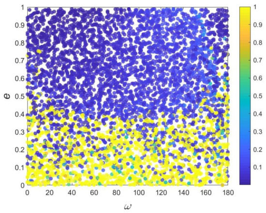
Figure 1. The lifetime of 5000 particles in 2/1 polar resonance on $e-\omega$ plane. The color bar represents the ratio of the lifetime of the particle and whole integration time span.

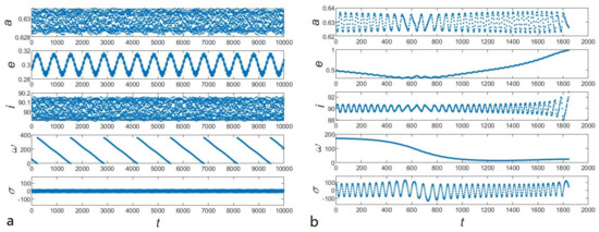
Figure 2. Dynamical evolution of the representatives of the surviving (plane (a)) and dead (plane (b)) particles. From top to bottom panel: semi-major axis a, eccentricity e, inclination i, argument of pericenter $\omega$, $2/1$ critical angle $\sigma$, respectively.

4.2. Phase-Space Structure of Polar $2/1$ Resonance

The resonant dynamics are the basis for our research on the secular mechanism inside MMRs. However, the polar resonant configurations have remained unclear until now. Let us first investigate the essential dynamical maps of polar MMRs, including the libration centers and resonant width. In Section 2.1, we introduce a set of canonical action-angles and explain that $a-\sigma$ phase-space portraits can understand the resonant dynamics well. Given the particular set of ($e,\omega$), the averaged Hamiltonian can be calculated in the $a-\sigma$ plane by Equation (4). Figure 3 shows three examples of phase-space portraits of polar $2/1$ resonance with a different set of ($e,\omega$), including the low- (panel a), medium- (panel b), and high-eccentric case (panel c).

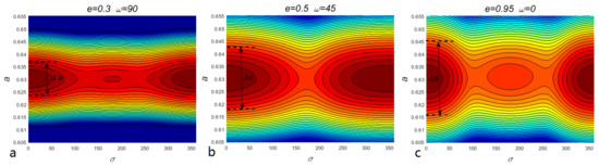
Figure 3. Phase-space portraits of $2/1$ polar resonance in $a-\sigma$ plane under three different sets of parameters $(e,\omega )$ (plane (a): $e=0.3,\omega ={90}^{\circ }$; plane (b): $e=0.5,\omega ={45}^{\circ }$; plane (c): $e=0.95,\omega =0^{\circ }$). The variances of the color and contours represent the level of the averaged Hamiltonian in Equation (4). $\Delta a$ is the resonant width of dominated libration center.

As shown in Figure 3, the positions corresponding to the minimum Hamiltonian is the resonant equilibriums. The resonant width $\Delta a$ is defined by the librational amplitude around the resonant equilibrium. Then, we can obtain the resonant equilibriums and width of the resonance $\Delta a$. Here, we define the dominated resonant equilibrium as the center with the larger resonant width. For the cases which have more than one equilibrium, such as panels a and c in Figure 3, the resonant width $\Delta a$ refers to the larger one. Therefore, all of the dominated libration centers of four cases depicted in Figure 3 are $\sigma =0^{\circ }$. For each set of the grid on the $e-\omega$ plane, we plot the phase-space portrait and disturbing function as in Figure 3. Then, we can obtain the dominated libration centers and resonant width $\Delta a$ for each set of $(e,\omega )$. Figure 4 systematically presents the polar $2/1$ resonant dynamical map, including resonant libration center and resonant width. The alpha of markers represents the resonant width, and the color indicates its dominated libration center. The dominated libration centers of polar $2/1$ resonance are always around $\sigma =0^{\circ }$ for all the sets of $(e,\omega )$, which provides an essential guide for our further study of the Kozai mechanism in polar $2/1$ resonance. This is the first time that the dynamics of polar $2/1$ resonance have been systematically studied.

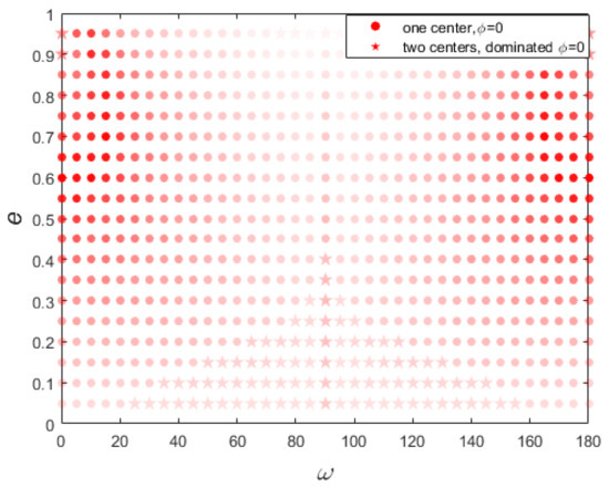
Figure 4. The scatter map of the resonant width of polar $2/1$ resonance on the $e-\omega$ plane. The filled dots and pentagons represent their corresponding phase-space portraits that have one or two equilibriums, respectively. The color reflects the position of the libration center. The red means that the dominated libration center is around $\sigma =0^{\circ }$. In other cases, such as interior $2/3$ resonance we will introduce later, there is a blue part, which means its dominated resonant equilibrium is around $\sigma ={180}^{\circ }$. The alpha of the marker represents the resonant width under the corresponding parameters. The higher the transparency, the narrower the resonant width.

4.3. Kozai–Lidov Dynamics inside Polar 2/1 Resonance

In our numerical experiments, as shown in Figure 1, resonant particles have a different destiny, The secular dynamics inside MMR need to be considered to explain the results of our numerical experiments. As we have introduced in Section 2.2, the secular dynamics on the $e-\omega$ space can be obtained simply by the set $a=a_0$. It has been confirmed that all the dominated resonant equilibriums are around $\sigma =0^{\circ }$ for the polar $2/1$ resonance. If we consider the exact resonance case, the resonant angle is always equal to $\sigma =0^{\circ }$. The averaged Hamiltonian can be calculated by Equation (5). If we consider the effect of libration amplitude ${\sigma }_{\mathrm{amp}}$ of the resonant angle, the averaged Hamiltonian is given by Equation (6). The phase-space portraits in three different resonant amplitudes (${\sigma }_{\mathrm{amp}}=0^{\circ },{60}^{\circ },{150}^{\circ }$) are depicted in Figure 5. Comparing these three portraits, we know that the effects of libration amplitude can be ignored when the libration amplitude is small. Dynamical evolutions of several representative particles in numerical integrations are also plotted in panel a. The solid black dots represent the initial positions of test particles, and the arrows depict the evolution of unstable particles in numerical integrations. The numerical results correspond very well with the level curves of the Hamiltonian. Therefore, we use the $e-\omega$ portrait at exact resonance to analyze the Kozai mechanism directly. The most typical dynamics reflected by the $e-\omega$ portrait under exact $2/1$ polar resonance are as follows: Firstly, for the high-eccentric region (around $e>0.5$), the $\omega$ is limited to oscillations while the eccentricity will rise to around 1. Therefore, the particles in this high-eccentric region should be unstable. Instead, the variations in eccentricity are maintained within a small range, and the $\omega$ is in circulation in the lower eccentricity region. Therefore, the particles in the low-eccentric region should have long-term stability.

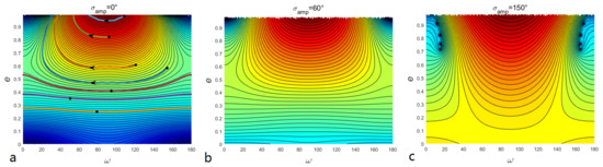
Figure 5. Phase-space portraits of Kozai–Lidov dynamics inside the polar $2/1$ resonance. The levels of Hamiltonian in Equation (5) or (6) are plotted on an $e-\omega$ plane. The panels (a–c) represent three different cases (${\sigma }_{\mathrm{amp}}=0^{\circ },{60}^{\circ },{150}^{\circ }$). The thick colored solid lines in panel a represent the several representative results of numerical integrations. The solid black dots mark the positions of initial parameters and the arrows indicate the evolution direction of the dying particles.

As some assumptions are made to obtain the one d.o.f approximation of this problem, the validity of the $e-\omega$ portraits above should be checked by the numerical experiments. Comparing Figure 1, Figure 2, and Figure 5, the secular dynamics given by $e-\omega$ can explain the dynamical evolution of the test particles in the numerical experiments (the existence of some dead particles in the low-eccentric region can be understood by considering the effects of resonant amplitude ${\sigma }_{\mathrm{amp}}$), and thus the $e-\omega$ portraits can represent the real Kozai–Lidov dynamics inside polar $2/1$ resonance.

We have investigated the secular dynamics inside polar $2/1$ resonance using numerical integrations and the semi-analytical method by mutual authenticating. As a supplement, we study the purely polar secular dynamics further to discuss the effects of polar $2/1$ resonance. In our numerical experiments, the maximum libration width of polar $2/1$ resonance is no more than 0.05 au. We repeat the numerical integrations in Section 4.1 with initial semi-major axis $a=a_0+0.05$ while leaving the other parameters unchanged. The lifetime of 5000 particles is depicted in the left panel of Figure 6. We have checked that all of the particles are not in $2/1$ resonance with perturber. Similarly, the Hamiltonian can be calculated by numerical averaging all the fast angles $\lambda$ and ${\lambda }^{\prime }$ as follows:

$${\overline{\mathcal{H}}}_{\mathrm{pure}}=-\frac{\mu }{4{\pi }^{2}k}{\int }_0^{2\pi }{\int }_0^{2\pi }\left(\frac{1}{|r-r^{\prime }|}-\frac{r·r^{\prime }}{|r^{\prime }{|}^3}\right){|}_{a=a_0+0.05}\mathrm{d}{\lambda }^{\prime }\mathrm{d}\lambda .$$

(7)

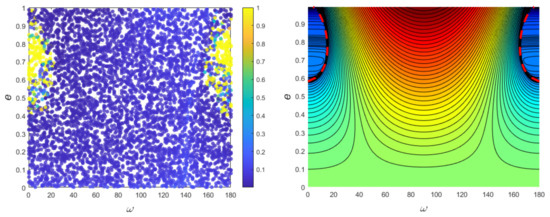
Figure 6. Pure secular dynamics of polar orbits outside the $2/1$ resonance. (Left panel): The lifetime ratio of the 5000 particles in numerical integrations. (Right panel): Phase-space portrait of pure secular dynamics. The levels of Hamiltonian in Equation (7) are plotted on $e-\omega$ plane. The thick black dashed lines denote collision curves with the perturber.

The pure secular dynamics in the $e-\omega$ portrait are shown in the right panel in Figure 6. The dynamics illustrated by the two panels of Figure 6 are in good agreement. Except for the regions within the collision curve, the eccentricity goes up to 1 and dies out in long-term evolution, entirely different from secular dynamics inside polar $2/1$ resonance. Comparing the results of Figure 1, Figure 5, and Figure 6, it is clear that the influence of polar $2/1$ resonance on secular dynamics is not negligible.

So far, taking the classical $2/1$ resonance as an example, we have systematically studied the polar interior resonance in the model of CRTBP. As a supplement, we analyze the pure secular dynamics of polar orbits outside the $2/1$ resonance and compare them with the resonant secular dynamics. The importance of polar $2/1$ resonance to the long-term dynamics is demonstrated.

5. Dynamics of Exterior Polar Resonance, the $2/3$ Case

Now, we focus on the dynamics of exterior polar resonance except $1/n$ resonance (n are positive integers), taking $2/3$ as an example. Since the methods are similar to interior resonance, we mainly present relevant conclusions here.

The polar $2/3$ resonant configuration is depicted in Figure 7. The most obvious difference from the $2/1$ resonance (Figure 4) is the emergence of the dominated resonant equilibriums at $\sigma ={180}^{\circ }$ (corresponding to the blue part in Figure 7) for $2/3$ resonance. For the high-eccentric region where $e>0.7$, the dominated resonant equilibriums have libration centers at $\sigma =0^{\circ }$, while in other cases the dominated libration centers are at $\sigma ={180}^{\circ }$. Therefore, when we analyze the Kozai–Lidov dynamics inside polar $2/3$ resonance, both of the $e-\omega$ portraits at $\sigma =0^{\circ }$ and $\sigma ={180}^{\circ }$ are required. Figure 8 depicts the lifetime of 5000 particles in numerical experiments (panel a), and Kozai–Lidov dynamics inside exact polar $2/3$ resonance with $\sigma =0^{\circ }$ (panel b) and with $\sigma ={180}^{\circ }$ (panel c). As shown in panels b and c of Figure 8, the evolutions of several particles in numerical integrations are depicted and correspond very well with the $e-\omega$ portraits. Like the numerical results of $2/1$ resonance, almost all 5000 particles are trapped in polar $2/3$ resonance with the perturber. The unstable particles die due to their eccentricities rising to 1. Combining Figure 7 and Figure 8, the secular dynamics inside polar $2/3$ resonance should be understood as follows: For the region with eccentricity $e<0.7$ where their dominated resonance is around $\sigma ={180}^{\circ }$, their Kozai–Lidov dynamics are described by the corresponding region ($e<0.7$) in panel c of Figure 8. The $\omega$ is circulation, and eccentricity is limited to a small range of oscillations, so particles in this region are stable in numerical experiments (see panel a of Figure 8). Conversely, for the high-eccentric region ($e>0.7$) where their dominated resonant equilibriums are at $\sigma =0^{\circ }$, their secular dynamics should be understood by the corresponding region ($e>0.7$) in panel b of Figure 8. For the extreme high-eccentric region, the $\omega$ oscillates while eccentricity rises to 1 and leads to instability. The Kozai–Lidov dynamics inside $2/3$ resonance described by $e-\omega$ portraits can explain the numerical phenomena. This further verifies that the phase-space portraits from the semi-analytical method represent the real secular dynamics inside resonance. As shown in Figure 8a, there appear to be several low-eccentricity particles ($e\le 0.4$) with very short lifetimes. The dynamical evolution of these atypical particles is depicted in Figure 9. There are two noteworthy features: The eccentricity increases rapidly to 1 and dies out; the critical angle’s libration center goes from $0^{\circ }$ to ${180}^{\circ }$. Naturally, this phenomenon cannot be explained by the phase-space portraits with a certain libration center $0^{\circ }$ or ${180}^{\circ }$ (Figure 8b,c). We will try to make this complicated evolution clear in our future work.

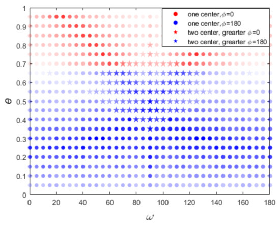
Figure 7. Same as Figure 4, but for polar $2/3$ resonance.

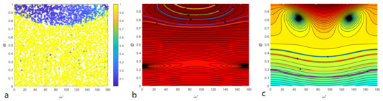
Figure 8. (a) Same as Figure 1, but for polar $2/3$ resonance. Panel (b,c) are phase-space portraits of Kozai–Lidov dynamics on $e-\omega$ plane under exact $2/3$ resonance with libration center $\sigma =0^{\circ }$ and $\sigma ={180}^{\circ }$, respectively. The thick colored solid lines represent the numerical results. The solid black dots mark the initial positions of particles, and the arrows indicate the evolution direction of unstable particles.

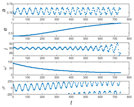
Figure 9. The dynamical evolution of these atypical particles (unstable particles with low eccentricity) in Figure 8a.

We have also investigated the dynamics of other exterior polar resonances, such as $2/5$, $7/9$. They have similar resonant secular dynamics with $2/3$ resonance. As for the exterior polar $1/n$ resonances, considering the effect of asymmetric libration ($\sigma$ librates neither $0^{\circ }$ nor ${180}^{\circ }$) [88,89,90], there will be some new challenges that need further discussion. We will try to investigate the dynamics of polar $1/n$ resonance in our next work.

6. Conclusions

In this paper, we study the dynamical maps of polar resonance and its effect on the Kozai–Lidov mechanism in the context of CRTBP using numerical and semi-analytical methods by mutual authenticating. Previous studies on resonance paid little attention to the perpendicular orbits with inclination $i={90}^{\circ }$. We introduce the action-angle variables for polar resonances and deduce proper canonical transformations. We can calculate the Hamiltonian by averaging over the fast angles and plot the level curves of the Hamiltonian on a $e-\omega$ space, which can be used to understand the Kozai–Lidov dynamics inside polar resonance.

Then, we analyze the polar resonant dynamics of interior and exterior resonances, taking the $2/1$ and $2/3$ resonances as examples. The resonant libration centers and width are studied for each case. The most apparent difference in dynamics of $2/1$ and $2/3$ resonance is their libration centers. As shown in Figure 4 and Figure 7, the dominated libration centers are always at $\sigma =0^{\circ }$ for $2/1$ resonance, while the centers around $\sigma ={180}^{\circ }$ appear in $2/3$ resonance. The determination of the resonance center provides the basis for the following semi-analytical work. The Kozai–Lidov dynamics inside polar resonance are depicted on the $e-\omega$ space as shown in Figure 5 and Figure 8. Evolutions of several representative particles are also depicted and correspond very well with level curves with Hamiltonian. We confirm that the moderate libration amplitude of critical angle ${\sigma }_{\mathrm{amp}}$ has no pronounced effect on $e-\omega$ portraits. The lifetime of 5000 particles in resonance are investigated by numerical integrations in Figure 1 and Figure 8. All of the dead particles are due to their eccentricities rising to 1. The $e-\omega$ spaces can explain the numerical performances for interior and exterior polar resonances, which demonstrates that the $e-\omega$ spaces represent the real Kozai–Lidov dynamics inside polar resonances. These phase-space portraits of the Kozai–Lidov mechanism can be used to investigate the long-term evolution of polar resonant particles. As a supplement, we study the pure secular dynamics outside polar $2/1$ resonance, and demonstrate that we cannot ignore the effect of polar resonance on secular dynamics. In this way, we can also study other resonant secular dynamics. Our work can be used to understand the dynamics of minor bodies that are in polar resonance with the planet. It may also help to look for objects with polar orbits in the resonant region of the planet. We will investigate the dynamics of exterior polar $1/n$ resonance where the asymmetric librations may exist in our next work.

References

- Henrard, J. A note concerning the 2:1 and the 3:2 resonances in the asteroid belt. Celest. Mech. Dyn. Astron. 1996, 64, 107–114. [Google Scholar] [CrossRef]
- Malhotra, R. The Phase Space Structure Near Neptune Resonances in the Kuiper Belt. Astron. J. 1996, 111, 504. [Google Scholar] [CrossRef]
- Sokolov, L.L.; Bashakov, A.A.; Pit’Ev, N.P. Resonance orbits of near-Earth asteroids. Sol. Syst. Res. 2009, 43, 319–323. [Google Scholar] [CrossRef]
- Smirnov, E.A.; Dovgalev, I.S.; Popova, E.A. Asteroids in three-body mean motion resonances with planets. Icarus 2018, 304, 24–30. [Google Scholar] [CrossRef]
- Malhotra, R.; Lan, L.; Volk, K.; Wang, X. Neptune’s 5:2 Resonance in the Kuiper Belt. Astron. J. 2018, 156, 55. [Google Scholar] [CrossRef]
- Harris, A.W.; D Abramo, G. The population of near-Earth asteroids. Icarus 2015, 257, 302–312. [Google Scholar] [CrossRef]
- Qi, Y.; de Ruiter, A. Planar near-Earth asteroids in resonance with the Earth. Icarus 2019, 333, 52–60. [Google Scholar] [CrossRef]
- Li, M.; Huang, Y.; Gong, S. Assessing the risk of potentially hazardous asteroids through mean motion resonances analyses. APSS 2019, 364, 78. [Google Scholar] [CrossRef]
- Nesvorný, D.; Thomas, F.; Ferraz-Mello, S.; Morbidelli, A. A perturbative treatment of the co-orbital motion. Celest. Mech. Dyn. Astron. 2002, 82, 323–361. [Google Scholar] [CrossRef]
- Peale, S.J. Orbital resonance in the solar system. Annu. Rev. Astron. Astrophys. 1976, 14, 215–246. [Google Scholar] [CrossRef]
- Nesvorny, D.; Ferraz-Mello, S. On the Asteroidal Population of the First-Order Jovian Resonances. Nature 1997, 130, 247–258. [Google Scholar] [CrossRef]
- Murray, C.D.; Dermott, S.F. Solar System Dynamics; Cambridge University Press: Cambridge, UK, 1999. [Google Scholar]
- Morbidelli, A. Modern Celestial Mechanics: Aspects of Solar System Dynamics; CRC Press: Boca Raton, FL, USA, 2002. [Google Scholar]
- Gallardo, T. Atlas of the mean motion resonances in the Solar System. Icarus 2006, 184, 29–38. [Google Scholar] [CrossRef]
- Gallardo, T. Strength, stability and three dimensional structure of mean motion resonances in the solar system. Icarus 2019, 317, 121–134. [Google Scholar] [CrossRef]
- Namouni, F.; Morais, M.H.M. Resonance capture at arbitrary inclination. Mon. Not. R. Astron. Soc. 2015, 446, 1998–2009. [Google Scholar] [CrossRef]
- Namouni, F.; Morais, M.H. Resonance capture at arbitrary inclination—II. Effect of the radial drift rate. Mon. Not. R. Astron. Soc. 2017, 467, 2673–2683. [Google Scholar] [CrossRef][Green Version]
- Morais, M.H.M.; Namouni, F. Retrograde resonance in the planar three-body problem. Celest. Mech. Dyn. Astron. 2013, 117, 405–421. [Google Scholar] [CrossRef]
- Morais, M.H.M.; Namouni, F. A numerical investigation of coorbital stability and libration in three dimensions. Celest. Mech. Dyn. Astron. 2016, 125, 91–106. [Google Scholar] [CrossRef]
- Wiegert, P.; Connors, M.; Veillet, C. A retrograde co-orbital asteroid of Jupiter. Nature 2017, 543, 687–689. [Google Scholar] [CrossRef]
- Huang, Y.; Li, M.; Li, J.; Gong, S. Dynamic portrait of the retrograde 1:1 mean motion resonance. Astron. J. 2018, 155, 262. [Google Scholar] [CrossRef]
- Namouni, F.; Morais, M.H. An interstellar origin for Jupiter’s retrograde co-orbital asteroid. Mon. Not. R. Astron. Soc. 2018, 477, L117–L121. [Google Scholar] [CrossRef]
- Li, M.; Huang, Y.; Gong, S. Centaurs potentially in retrograde co-orbit resonance with Saturn. Astron. Astrophys. 2018, 617, A114. [Google Scholar] [CrossRef]
- Morais, M.H.M.; Namouni, F. Periodic orbits of the retrograde coorbital problem. Mon. Not. R. Astron. Soc. 2019, 490, 3799–3805. [Google Scholar] [CrossRef]
- Li, M.; Huang, Y.; Gong, S. Survey of asteroids in retrograde mean motion resonances with planets. Astron. Astrophys. 2019, 630, A60. [Google Scholar] [CrossRef]
- Lei, H. Three-dimensional phase structures of mean motion resonances. Mon. Not. R. Astron. Soc. 2019, 487, 2097–2116. [Google Scholar] [CrossRef]
- Gallardo, T. Three-dimensional structure of mean motion resonances beyond Neptune. Celest. Mech. Dyn. Astron. 2020, 132, 1–26. [Google Scholar] [CrossRef]
- Namouni, F.; Morais, M.H.M. Resonance libration and width at arbitrary inclination. Mon. Not. R. Astron. Soc. 2020, 493, 2854–2871. [Google Scholar] [CrossRef]
- Lidov, M. The evolution of orbits of artificial satellites of planets under the action of gravitational perturbations of external bodies. Planet. Space Sci. 1962, 9, 719–759. [Google Scholar] [CrossRef]
- Kozai, Y. Secular Perturbations of Asteroids with High Inclination and Eccentricity. Astron. J. 1962, 67, 579. [Google Scholar] [CrossRef]
- Shevchenko, I.I. The Lidov-Kozai Effect—Applications in Exoplanet Research and Dynamical Astronomy; Springer: Berlin, Germany, 2017. [Google Scholar]
- Innanen, K.; Zheng, J.; Mikkola, S.; Valtonen, M. The Kozai Mechanism and the Stability of Planetary Orbits in Binary Star Systems. Astron. J. 1997, 113, 1915. [Google Scholar] [CrossRef]
- Jianghui, J.; Kinoshita, H.; Lin, L.; Guangyu, L.; Nakai, H. The Stability Analysis of the HD 82943 and HD 37124 Planetary Systems. arXiv 2002, arXiv:astro–ph/0208025. [Google Scholar]
- Wen, L. On the Eccentricity Distribution of Coalescing Black Hole Binaries Driven by the Kozai Mechanism in Globular Clusters. Astrophys. J. 2003, 598, 419–430. [Google Scholar] [CrossRef]
- Funk, B.; Libert, A.S.; Süli, Á.; Pilat-Lohinger, E. On the influence of the Kozai mechanism in habitable zones of extrasolar planetary systems. Astron. Astrophys. 2011, 526, A98. [Google Scholar] [CrossRef]
- De La Fuente Marcos, C.; de La Fuente Marcos, R. Extreme trans-Neptunian objects and the Kozai mechanism: Signalling the presence of trans-Plutonian planets. Mon. Not. R. Astron. Soc. 2014, 443, L59–L63. [Google Scholar] [CrossRef]
- Bailey, M.E.; Chambers, J.E.; Hahn, G. Origin of sungrazers - A frequent cometary end-state. Astron. Astrophys. 1992, 257, 315–322. [Google Scholar]
- Thomas, F.; Morbidelli, A. The Kozai resonance in the outer solar system and the dynamics of long-period comets. Celest. Mech. Dyn. Astron. 1996, 64, 209–229. [Google Scholar] [CrossRef]
- Lei, H. A semi-analytical model for secular dynamics of test particles in hierarchical triple systems. Mon. Not. R. Astron. Soc. 2019, 490, 4756–4769. [Google Scholar] [CrossRef]
- Naoz, S.; Farr, W.M.; Lithwick, Y.; Rasio, F.A. Hot Jupiters from secular planet-planet interactions. Nature 2011, 473, 187–189. [Google Scholar] [CrossRef]
- Naoz, S.; Farr, W.M.; Lithwick, Y.; Rasio, F.A. Secular dynamics in hierarchical three-body systems. Mon. Not. R. Astron. Soc. 2013, 431, 2155–2171. [Google Scholar] [CrossRef]
- Li, G.; Naoz, S.; Holman, M.; Loeb, A. Chaos in the test particle eccentric Kozai-Lidov mechanism. Astrophys. J. 2014, 791. [Google Scholar] [CrossRef]
- Naoz, S.; Li, G.; Zanardi, M.; de Elía, G.C.; Di Sisto, R.P. The Eccentric Kozai-Lidov Mechanism for Outer Test Particle. Astron. J. 2017, 154, 18. [Google Scholar] [CrossRef]
- Will, C. Orbital flips in hierarchical triple systems: Relativistic effects and third-body effects to hexadecapole order. Phys. Rev. D 2017, 96, 1–15. [Google Scholar] [CrossRef]
- Saillenfest, M.; Fouchard, M.; Tommei, G.; Valsecchi, G.B. Non-resonant secular dynamics of trans-Neptunian objects perturbed by a distant super-Earth. Celest. Mech. Dyn. Astron. 2017, 129, 329–358. [Google Scholar] [CrossRef]
- Kozai, Y. Secular perturbations of resonant asteroids. Celest. Mech. Dyn. Astron. 1985, 36, 47–69. [Google Scholar] [CrossRef]
- Giacaglia, G.E.O. Secular Motion of Resonant Asteroids. SAO Spec. Rep. 1968, 278, 47–69. [Google Scholar]
- Giacaglia, G.E.O. Resonance in the Restricted Problem of Three Bodies. Astron. J. 1969, 74, 1254. [Google Scholar] [CrossRef]
- Gomes, R.S.; Gallardo, T.; Fernandez, J.; Brunini, A. On the origin of the high-perihelion scattered disk: The role of the kozai mechanism and mean motion resonances. Celest. Mech. Dyn. Astron. 2005, 91, 109–129. [Google Scholar] [CrossRef]
- Gomes, R.S. The origin of TNO 2004 XR190 as a primordial scattered object. Icarus 2011, 215, 661–668. [Google Scholar] [CrossRef]
- Gallardo, T.; Hugo, G.; Pais, P. Survey of Kozai dynamics beyond Neptune. Icarus 2012, 220, 392–403. [Google Scholar] [CrossRef]
- Morbidelli, A.; Moons, M. Secular Resonances in Mean Motion Commensurabilities: The 2/1 and 3/2 Cases. Icarus 1993, 102, 316–332. [Google Scholar] [CrossRef]
- Moons, M.; Morbidelli, A. Secular Resonances in Mean Motion Commensurabilities: The 4/1, 3/1, 5/2, and 7/3 Cases. Icarus 1995, 114, 33–50. [Google Scholar] [CrossRef]
- Morbidelli, A.; Thomas, F.; Moons, M. The Resonant Structure of the Kuiper Belt and the Dynamics of the First Five Trans-Neptunian Objects. Icarus 1995, 118, 322–340. [Google Scholar] [CrossRef]
- Wan, X.S.; Huang, T.Y. An exploration of the Kozai resonance in the Kuiper Belt. Mon. Not. R. Astron. Soc. 2007, 377, 133–141. [Google Scholar] [CrossRef]
- Sidorenko, V.V.; Neishtadt, A.I.; Artemyev, A.V.; Zelenyi, L.M. Quasi-satellite orbits in the general context of dynamics in the 1:1 mean motion resonance: Perturbative treatment. Celest. Mech. Dyn. Astron. 2014, 120, 131–162. [Google Scholar] [CrossRef]
- Giuppone, C.A.; Leiva, A.M. Secular models and Kozai resonance for planets in coorbital non-coplanar motion. Mon. Not. R. Astron. Soc. 2016, 460, 966–979. [Google Scholar] [CrossRef]
- Saillenfest, M.; Fouchard, M.; Tommei, G.; Valsecchi, G.B. Long-term dynamics beyond Neptune: Secular models to study the regular motions. Celest. Mech. Dyn. Astron. 2016, 126, 369–403. [Google Scholar] [CrossRef]
- Saillenfest, M.; Fouchard, M.; Tommei, G.; Valsecchi, G.B. Study and application of the resonant secular dynamics beyond Neptune. Celest. Mech. Dyn. Astron. 2017, 127, 477–504. [Google Scholar] [CrossRef]
- Saillenfest, M.; Lari, G. The long-term evolution of known resonant trans-Neptunian objects. Astron. Astrophys. 2017, 79, 1–9. [Google Scholar] [CrossRef][Green Version]
- Batygin, K.; Morbidelli, A. Dynamical Evolution Induced by Planet Nine. Astron. J. 2017, 154, 229. [Google Scholar] [CrossRef]
- Sidorenko, V.V. Dynamics of “jumping” Trojans: A perturbative treatment. Celest. Mech. Dyn. Astron. 2018, 130, 1–18. [Google Scholar] [CrossRef]
- Tsiganis, K.; Dvorak, R.; Pilat-Lohinger, E. Thersites: A ’jumping’ Trojan? Astron. Astrophys. 2000, 354, 1091–1100. [Google Scholar]
- Huang, Y.; Li, M.; Li, J.; Gong, S. Kozai-Lidov mechanism inside retrograde mean motion resonances. Mon. Not. R. Astron. Soc. 2018, 481, 5401–5410. [Google Scholar] [CrossRef]
- Qi, Y.; de Ruiter, A. Kozai mechanism inside mean motion resonances in the three-dimensional phase space. Mon. Not. R. Astron. Soc. 2020, 493, 5816–5824. [Google Scholar] [CrossRef]
- Efimov, S.S.; Sidorenko, V.V. An analytically treatable model of long-term dynamics in a mean motion resonance with coexisting resonant modes. Celest. Mech. Dyn. Astron. 2020, 132, 1–38. [Google Scholar] [CrossRef]
- Batygin, K.; Brown, M.E. Generation of Highly Inclined Trans-Neptunian Objects by Planet Nine. Astrophys. J. 2016, 833, L3. [Google Scholar] [CrossRef]
- Namouni, F.; Morais, M.H. The disturbing function for asteroids with arbitrary inclinations. Mon. Not. R. Astron. Soc. 2016, 474, 157–176. [Google Scholar] [CrossRef]
- Morais, M.H.M.; Namouni, F. First trans-Neptunian object in polar resonance with Neptune. Mon. Not. R. Astron. Soc. 2017, 472, L1–L4. [Google Scholar] [CrossRef]
- Namouni, F.; Morais, M.H. The disturbing function for polar Centaurs and transneptunian objects. Mon. Not. R. Astron. Soc. 2017, 471, 2097–2110. [Google Scholar] [CrossRef]
- Jorba, À.; Masdemont, J. Dynamics in the center manifold of the collinear points of the restricted three body problem. Phys. D Nonlinear Phenom. 1999, 132, 189–213. [Google Scholar] [CrossRef]
- Masdemont, J. High-order expansions of invariant manifolds of libration point orbits with applications to mission design. Dyn. Syst. Int. J. 2005, 20, 59–113. [Google Scholar] [CrossRef]
- Hou, X.Y.; Liu, L. On motions around the collinear libration points in the elliptic restricted three-body problem. Mon. Not. R. Astron. Soc. 2011, 415, 3552–3560. [Google Scholar] [CrossRef][Green Version]
- Nesvorný, D.; Morbidelli, A. An analytic model of three-body mean motion resonances. Celest. Mech. Dyn. Astron. 1998, 71, 243–271. [Google Scholar] [CrossRef]
- Ellis, K. The Disturbing Function in Solar System Dynamics. Icarus 2000, 147, 129–144. [Google Scholar] [CrossRef]
- Mardling, R.A. New developments for modern celestial mechanics. I. General coplanar three-body systems. Application to exoplanets. Mon. Not. R. Astron. Soc. 2013, 435, 2187–2226. [Google Scholar] [CrossRef]
- Moons, M.; Morbidelli, A. The main mean motion commensurabilities in the planar circular and elliptic problem. Celest. Mech. Dyn. Astron. 1993, 57, 99–108. [Google Scholar] [CrossRef]
- Wang, X.; Malhotra, R. Mean Motion Resonances at High Eccentricities: The 2:1 and the 3:2 Interior Resonances. Astron. J. 2017, 154, 20. [Google Scholar] [CrossRef]
- Michtchenko, T.A.; Beaugé, C.; Ferraz-Mello, S. Dynamic portrait of the planetary 2/1 mean-motion resonance—II. Systems with a more massive inner planet. Mon. Not. R. Astron. Soc. 2008, 391, 215–227. [Google Scholar] [CrossRef]
- Michtchenko, T.A.; Beaugé, C.; Ferraz-Mello, S. Dynamic portrait of the planetary 2/1 mean-motion resonance—I. Systems with a more massive outer planet. Mon. Not. R. Astron. Soc. 2008, 387, 747–758. [Google Scholar] [CrossRef]
- Li, M.; Huang, Y.; Gong, S. Dynamics of retrograde 1/n mean motion resonances: The 1/-2, 1/-3 cases. Astrophys. Space Sci. 2020, 365, 1–13. [Google Scholar] [CrossRef]
- Gallardo, T. The occurrence of high-order resonances and Kozai mechanism in the scattered disk. Icarus 2006, 181, 205–217. [Google Scholar] [CrossRef]
- Li, J.; Zhou, L.Y.; Sun, Y.S. A study of the high-inclination population in the Kuiper belt—I. The Plutinos. Mon. Not. R. Astron. Soc. 2013, 437, 215–226. [Google Scholar] [CrossRef]
- Beaugé, C.; Roig, F. A Semianalytical Model for the Motion of the Trojan Asteroids: Proper Elements and Families. Icarus 2001, 153, 391–415. [Google Scholar] [CrossRef]
- Gallardo, T. Atlas of three body mean motion resonances in the Solar System. Icarus 2014, 231, 273–286. [Google Scholar] [CrossRef]
- Brasil, P.I.; Gomes, R.S.; Soares, J.S. Dynamical formation of detached trans-Neptunian objects close to the 2:5 and 1:3 mean motion resonances with Neptune. Astron. Astrophys. 2014, 564, 1–12. [Google Scholar] [CrossRef]
- Chambers, J.E. A hybrid symplectic integrator that permits close encounters between massive bodies. Mon. Not. R. Astron. Soc. 1999, 304, 793–799. [Google Scholar] [CrossRef]
- Message, P.J. Proceedings of the Celestial Mechanics Conference: The search for asymmetric periodic orbits in the restricted problem of three bodies. Astron. J. 1958, 63, 443. [Google Scholar] [CrossRef]
- Schubart, J. Long-Period Effects in Nearly Commensurable Cases of the Restricted Three-Body Problem. Sao Spec. Rep. 1964, 149, 1–36. [Google Scholar]
- Beaugé, C. Asymmetric librations in exterior resonances. Celest. Mech. Dyn. Astron. 1994, 60, 225–248. [Google Scholar] [CrossRef]
Publisher’s Note: MDPI stays neutral with regard to jurisdictional claims in published maps and institutional affiliations. |
© 2022 by the authors. Licensee MDPI, Basel, Switzerland. This article is an open access article distributed under the terms and conditions of the Creative Commons Attribution (CC BY) license (https://creativecommons.org/licenses/by/4.0/).