1. Introduction
Since the reform and opening up, the textile industry has always been a traditional pillar industry of the Chinese national economy, and it is also an industry with obvious international competitive advantages. It plays an important role in prospering the market, expanding exports, absorbing employment and promoting urbanization. In the process of fabric production, the inspection of fabric defects is a key factor in determining the quality of fabrics. The traditional artificial detection of fabric defects are generally inefficient, high cost and have a high detection error rate. If there have some defects in the surface of the fabric, then the cost price will increase by about 45–60% [
1], which will reduce the economic effect of the enterprise. Therefore, the textile industry is in urgent need of a new solution, such as an automatic fabric defect detection system, which can not only significantly reduce the detection time of the same batch of fabric compared to human-based detection, but also improve the detection rate of defects, reducing the operating cost of the enterprise, and improving the overall profit.
Research on the algorithm of automatic fabric detection has been ongoing for many years, and some relatively mature methods have already been published. Various texture backgrounds, differences in the production environment of enterprises, and classification of various fabric defects have always restricted the accuracy and speed of automatic detection of fabric defects. In recent years, experts and scholars have conducted research in this field, and many different detection methods have been produced. The three most mainstream categories of these methods are: spectrum analysis [
2,
3], model analysis [
4,
5] and deep learning-based methods [
6,
7,
8]. Although most industrial production currently uses the first two methods, the deep learning-based methods have greatly surpassed them in terms of detection speed and detection accuracy, and have begun to be applied to industrial fabric defect detection on a large scale.
Since its introduction, deep learning has been widely used in related research, such as in the medical field [
9,
10,
11,
12,
13], various types of target recognition [
14,
15,
16] and natural language processing [
17], and has achieved quite good results in these fields. Therefore, using the deep learning method to detect fabric defects will result in more accurate detection results.
In the aspect of using a basic deep learning model on fabric detection, Bu et al. [
18] proposed a data description model based on support vector; the optimal Gaussian kernel parameters are selected during training to solve the shortcomings of fabric defects that cannot be handled by a single fractal, however, this method is not particularly effective for image classification with strong textures. Huang et al. [
19] proposed an efficient convolutional neural network for defect segmentation and detection; this framework can significantly alleviate the amount of pictures needed while training the neural network and obtain the location of defects with high accuracy. The results show that this network significantly outperforms eight state-of-the-art methods in terms of accuracy and robustness. The methods introduced above use deep learning-based models. Although the detection effect is improved compared with the traditional methods, the basic deep learning model is incompetent for high-precision detection tasks such as Drone-captured Scenarios [
20], and the actual detection effect cannot meet the requirements of accurately locating defects.
Therefore, replacing the basic model with a classical model which has a more stable detection effect is the research direction in recent years. Wei et al. [
21] proposed a faster region-based convolutional neural network with a visual gain mechanism (Faster VG-RCNN). By analyzing the relationship between the attention mechanism and the visual gain mechanism, it was found that the attention-related visual gain mechanism can change the corresponding magnitude without changing the selectivity, and improve visual perception. Compared with Faster-RCNN, the experimental results show that the detection accuracy is improved by about 4%. Jing et al. [
22] proposed a fabric defect detection algorithm based on improved YOLOv3, first using the K-Means algorithm to determine the suitable anchors, then combining the low-level and high-level information, and adding the Yolo detection layer to the feature maps of different sizes. After the improvement, the false detection rate for specific types of fabric is less than 5%. Wang et al. [
23] proposed a fabric defect detection algorithm based on improved Yolov5. The Adaptive Spatial Feature Fusion (ASFF) method is used to improve the bad effect of Path Aggregation Network (PANet) on multi-scale features, and an attention mechanism is added to make the network focus on useful information. The final experimental results show that the average accuracy rate in fabric defect detection is 71.70%. Dlamini et al. [
24] proposed an improved YOLOv4 network: first, preprocess the flawed image to decompose the image into smaller sizes, and then use the filtering method to denoise the flawed features to enhance the robustness of the model, then deploy the trained model to the hardware; the accuracy of detecting specific flaws reached 95.3%. Kahraman et al. [
25] proposed a capsule Network, unlike the traditional CNN, which causes information loss, the capsules are capable of holding more information and are a group of neurons that include not only the probability of a particular object’s presence, but also different informative values related to instantiation parameters. The result shows the CapsNet achieved a performance value of 98.7%. Zheng et al. [
26] proposed SE-YOLOv5 network, adding the Squeeze-and-Excitation Networks (SE) [
27] module to the backbone network of YOLOv5 and replacing the ReLU activation function in the Cross Stage Partial (CSP) module with the Activate or Not (ACON) [
28] activation function. Experimental results show that the accuracy, generalization ability, and robustness are improved. After using the classic model and improving it, it can be seen that the accuracy of the detection results has been greatly improved, and the requirements of accurate positioning of defects can be achieved when detecting ordinary defect targets, however, when encountering tiny targets, the detection effect will be greatly reduced.
In the field of tiny target detection, Cui et al. [
29] proposed an improved YOLOv4 network to detect tiny targets in transmission line faults, adding an attention module combining ECAM (Efficient Channel Attention Module) and CBAM (Convolutional Block Attention Module) into the backbone network, using the clustering algorithm to regenerate Anchors, and, using a new loss function, the mAP50 for tiny target transmission line fault detection reaches 95.16%. Moran et al. [
30] improved the YOLOv3 network for tiny target prediction problems; the feature map output extracted by the second-layer residual network of the backbone is fused with the feature map output of other residual layers to form a new feature prediction layer, and the anchors are clustered using a clustering algorithm. Great results have been achieved in tiny target prediction from satellite image. Xu et al. [
31] proposed to add an attention mechanism and a feature extraction auxiliary network composed of multiple residual blocks. A smaller scale than the backbone network in the bypass of the original YOLOv3 backbone features extraction networks on the tiny target problem, then the auxiliary network will transfer the extracted location features to the backbone network to learn the detailed features of tiny targets more accurately. The mAP of tiny target detection in the car driving scene reaches 84.76%, Zhu et al. [
20]. In the tiny target detection for the drone-capture scenario, the TPH-YOLOv5 model is proposed. They add one more prediction head to detect different-scale objects, then use a Transformer Prediction Head (TPH) to replace the original prediction heads to excavate the prediction potential of the network; the results show this model is better than previous SOTA methods by 1.81%. The above models in their respective fields have made corresponding improvements to the structure of the model, according to the characteristics of the tiny targets in their own field datasets, so that the model can more accurately detect the tiny targets existing in the image. In the field of fabric defects, there are few model improvements specifically related to tiny targets.
Based on the above research, an improved YOLOv4 network is proposed to achieve accurate detection of tiny objects with fabric defects. The first step uses a new data augmentation method to expand the dataset to enhance the generalization ability of the model, the second step uses a clustering algorithm to cluster the augmented dataset and selects suitable yolo_anchors, the third step is to add a layer of feature detection specifically for tiny targets in the prediction network. The fourth step is to add a convolutional attention module to the backbone network to enhance the ability of the network to extract features. Finally, the loss function of the network is optimized to speed up the network convergence.
3. Methods
3.1. Data Augmentation
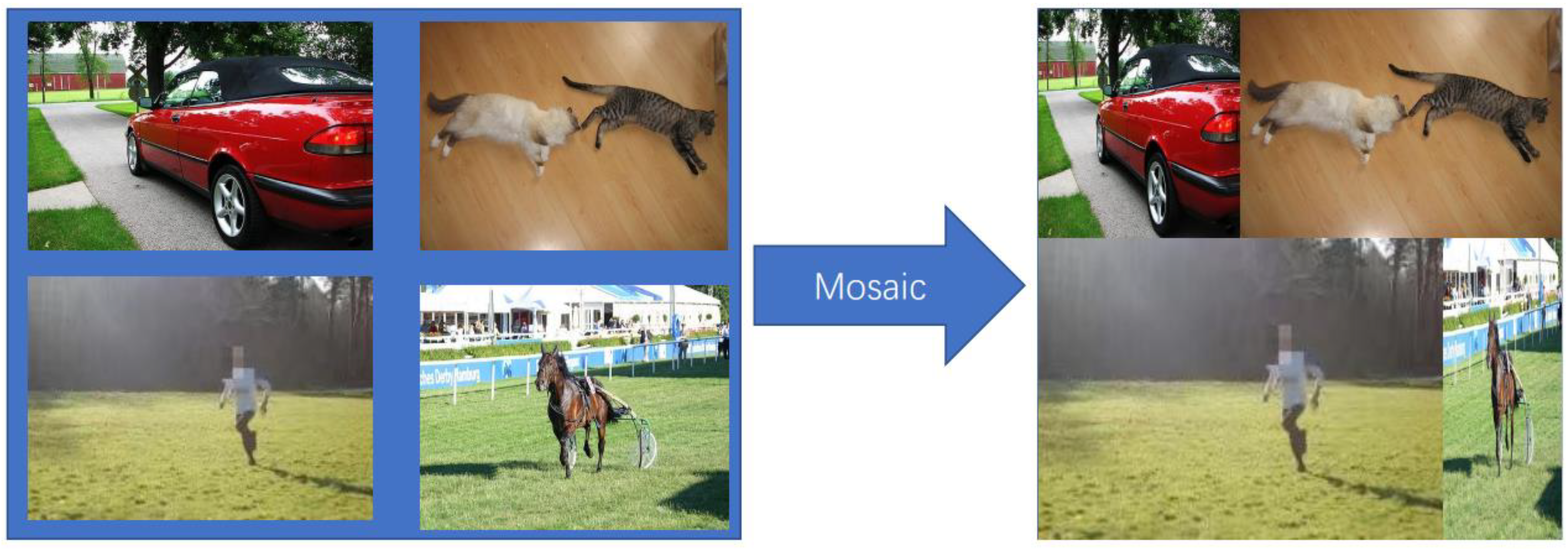
The YOLOv4 network uses Mosaic data augmentation at the input. The principle is to select 4 pictures in the dataset, and then place the four pictures in the four corners of a canvas after scaling, rotating and color gamut changes. The advantage is that this can enrich the background information of the entire detected object, and can calculate all the data of 4 pictures at the same time when calculating the picture. The Mosaic data augmentation is shown in
Figure 2.
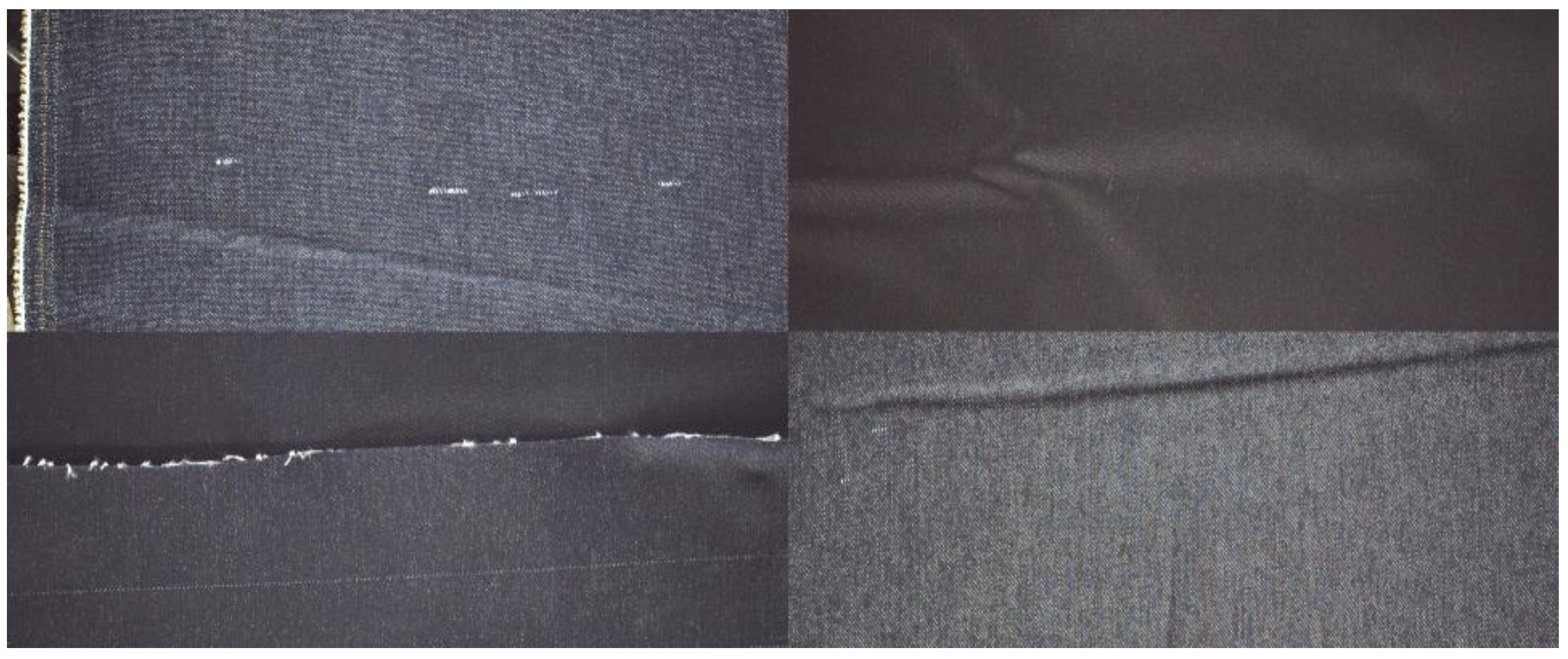
However, in the real production environment, there will be some very tiny targets such as knots and very large targets such as flower board jumps. In the case of 416 × 416 resolution, the real ground truth box of the tiny target is only about 6 × 6 on average, if Mosaic data enhancement is used to zoom the image, the already very small real frame will be compressed to a smaller size, which greatly hinders the network’s ability to detect such extremely small targets. At the same time, the average real frame of the extremely large target is Around 416 × 50, because the Mosaic dataset will crop the original image, this may make the network only train the local information of the large target and cannot pay attention to the global information of the large target.
Therefore, Mosaic data augmentation is no longer used in this paper, and a new data augmentation method that is more suitable for the dataset in this paper is proposed. Four augmentation methods are randomly selected among the 5 methods of impulse noise, Gaussian blur, mirror flip, Multiply and Affine. Four selected methods combined to work on one image simultaneously, enhance the original image N times, and also correspondingly transform the ground truth box in the original image; N is the number of enhancements for each image. Multiply is to multiply each pixel in the image by a preset value to make it look brighter or darker, and Affine is to zoom in, zoom out, move up and down, left and right, and rotate the original image.
After data augmentation, the network can learn more location features and pixel features that the original image does not have, and improve the robustness and accuracy of the network for tiny target detection.
3.2. New PredictionLayer for YOLO Head
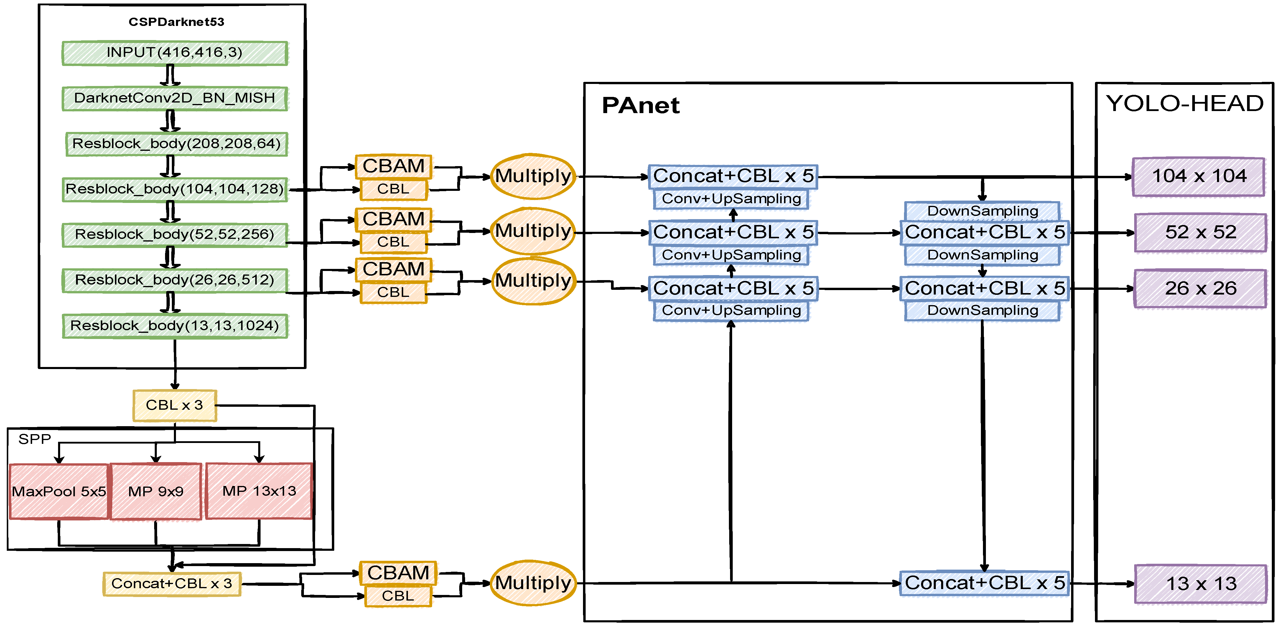
In the YOLOv4 network, after feature extraction, the backbone network will output three feature layers of different sizes, and then output to yolo_head for prediction after feature enhancement networks such as SPP and PANet. The sizes of these three feature layers are 13 × 13, 26 × 26, and 52 × 52; if the input image size is 416 × 416, the smallest pixel value that the network can detect is 8 × 8.
In the real production environment, there will be a large number of extremely tiny targets with an average ground truth box size of only 5 × 5, and if the size of the input image is too small, the YOLO network will automatically enlarge the image and add grayscale bars, but this will distort tiny objects in the image and interfere with the network’s ability to detect them.
In order to solve this kind of problem, this paper plans to add a layer of 104 × 104 feature output layer to change the minimum detection pixel value capability of the network to 4 × 4. The specific implementation method is that after the input image passes through the second Resblock_body of the CSPDarknet53 feature extraction network, not only outputting the extracted features to the next Resblock_body, but these output features are also fused with the features of other feature layers in PANet which have been processed by the CBL module and upsampling. The fused features will have richer semantic information, and then the feature layer will be downsampled and then passed down and fused with other feature layers. Finally, the feature layer of 104 × 104 will be output to yolo_head for prediction. Strengthening the network’s detection ability for extremely tiny targets, and improving the overall performance of the network for defect detection.
3.3. Attention Mechanism
CBAM [
40] (Convolutional Block Attention Module) consists of a Channel Attention Module and a Spatial Attention Module. These two modules strengthen effective feature information and suppress invalid information in the channel dimension and spatial dimension of deep features, respectively.
In the CBAM module, the input features first go through the channel attention module, and then the channel refined attention features will input into the spatial attention module, after that we will obtain the final refined features.
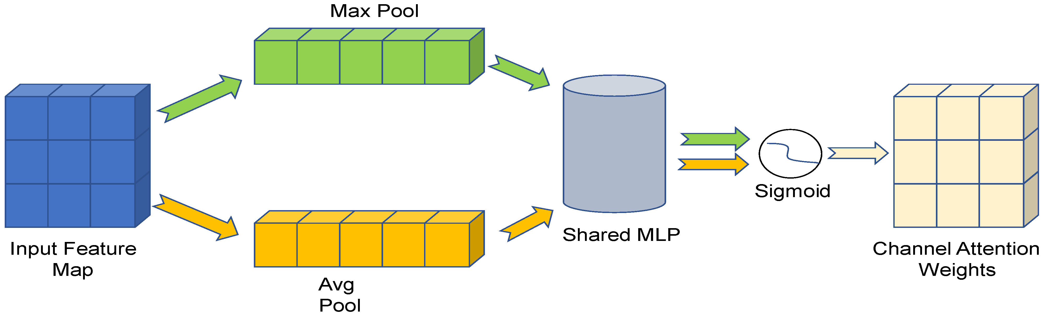
The structure of channel attention module is shown in
Figure 3.
Perform a maximum pooling and an average pooling operation on the input feature map in the spatial dimension, respectively, and then pass the pooled output through a shared weight MLP (multi-layer perceptron), and then also output the elements of the two outputs one by one. After the elements are added and passed through the sigmoid function, the channel attention weight is obtained. The formula of the channel attention module is shown in (1).
where
W1 and
W0 represent two convolution operations,
and
represent average pooling and maximum pooling at the channel level, respectively.
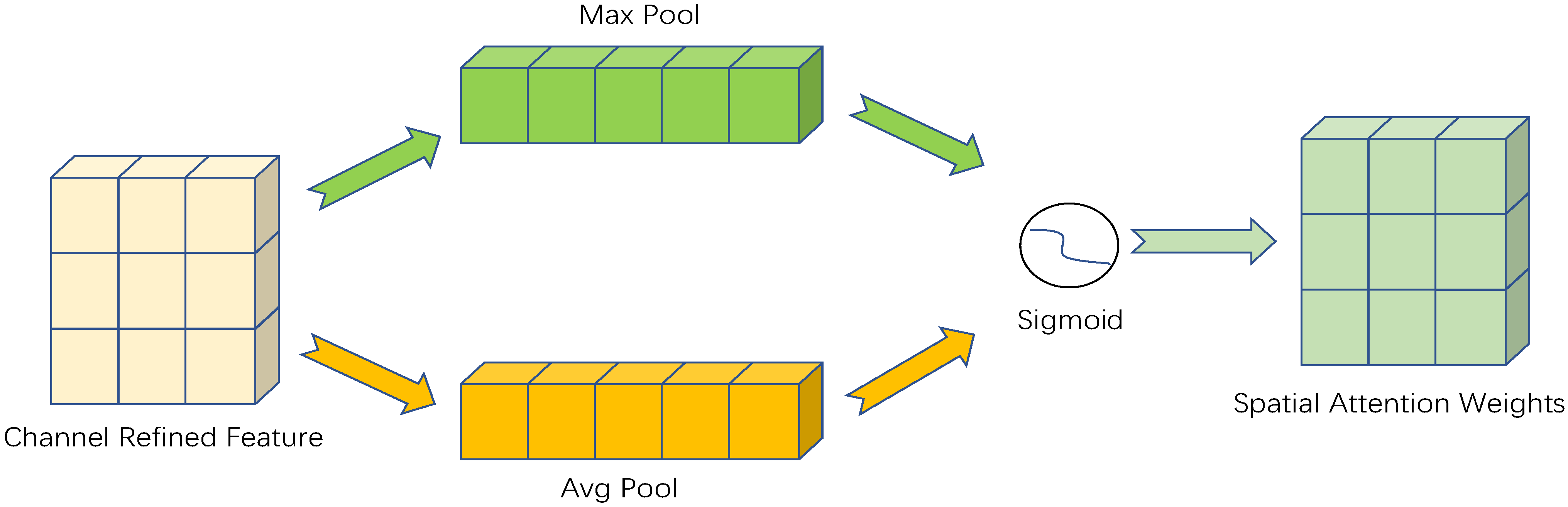
The structure of the spatial attention module is shown in
Figure 4.
Perform a maximum pooling and average pooling operations on each channel of the Channel refined feature map, and then concatenate those two pooled feature maps, convolution operations and sigmoid activation will be performed on the spliced feature maps. After the above operations, a spatial attention weight with a channel of 1 and the same size as the input feature map can be obtained; finally, an element-by-element multiplication with the input feature map is performed. The formula of the spatial attention module is shown in (2).
where
represents the sigmoid activation function,
represents the convolution kernel size is 7 × 7,
and
represent average pooling and maximum pooling at the spatial level, respectively.
In this paper, the convolutional attention module is integrated into the feature output layer of each dimension output by the CSPDarknet backbone network, and the output feature after spatial pyramid pooling. It makes the network pay more attention to key pixel features when predicting different feature layers, and improves the prediction accuracy of the network. The improved YOLOv4 network structure is shown in
Figure 5.
3.4. Clustering Anchors
In the prediction process of the original YOLOv4 network, each YOLO Head prediction feature layer corresponds to 3 priori boxes preset in the yolo_anchors file. Among them, the 9 default anchors in the yolo_anchors file are obtained by the author through clustering all the ground truth boxes in the VOC dataset. These 9 anchors are universal to most object detection situations and will not change in the process of training and prediction.
However, for this dataset, because the extremely tiny targets account for about 20% of all data, the accurate detection of the extremely tiny targets is an important indicator to test the improved network prediction effect. Because this paper adds a new feature layer to the original 3 prediction feature layers, the original yolo_anchors can no longer meet the needs of this experiment.
Therefore, this paper uses the K-means clustering algorithm to cluster the ground truth boxes in the augmented dataset, randomly select 12 points as the cluster center of the algorithm, calculates the similarity between each ground truth boxes and the cluster center, assigns these ground truth boxes to the cluster center with the closest similarity, calculates the mean of all samples in each cluster, and then updates the center of the cluster. Repeat the first two steps until the centers of the 12 clusters no longer change, or the maximum number of iterations set is reached, then the clustering ends, and the values of the 12 anchors we need are obtained.
The twelve Anchor values obtained in this paper using the K-means algorithm at multiple different feature layer scales are shown in
Table 1.
3.5. Optimized Loss Function
The loss function used in the YOLOv4 network is the Complete Intersection over union (CIOU) loss function. On the basis of DIOU, CIOU considers the aspect ratio of the detection frame into the loss function, and increases the aspect ratio influence factor , the accuracy of the frame regression has been further improved.
CIOU is represented by Equation (3).
IOU represents the intersection ratio between the ground truth box and the prediction box,
represents the Euclidean distance,
and
represent the center point of the ground truth box and the prediction box,
represents the diagonal distance of the smallest circumscribed rectangle,
is used to measure the consistency of the aspect ratio, and
is used to balance the value of
.
Although CIOU takes into account the overlapping area, the center point distance and aspect ratio of the frame regression, the aspect ratio difference reflected by in its formula is not the real difference between the width and height and its confidence.
Therefore, sometimes it will hinder the model from effectively optimizing the similarity and slow down the convergence speed of the model, so this paper replaces the CIOU with the EIOU which is more sensitive to the aspect ratio of the detection frame and has a faster convergence speed.
EIOU is represented by Equation (4),
is represented by Equation (5).
represents the width of the minimum bounding box covering the predicted box and the ground truth box,
represents the height of the minimum bounding box covering the predicted box and the ground truth box,
represents the width of the predicted box,
represents the width of the ground-truth box,
represents the height of the predicted box, and
represents the height of the ground-truth box.
When the value of EIOU is larger, it indicates that the overlap between the predicted box and the ground truth box is larger, the loss value is smaller, and the prediction result of the model is better.
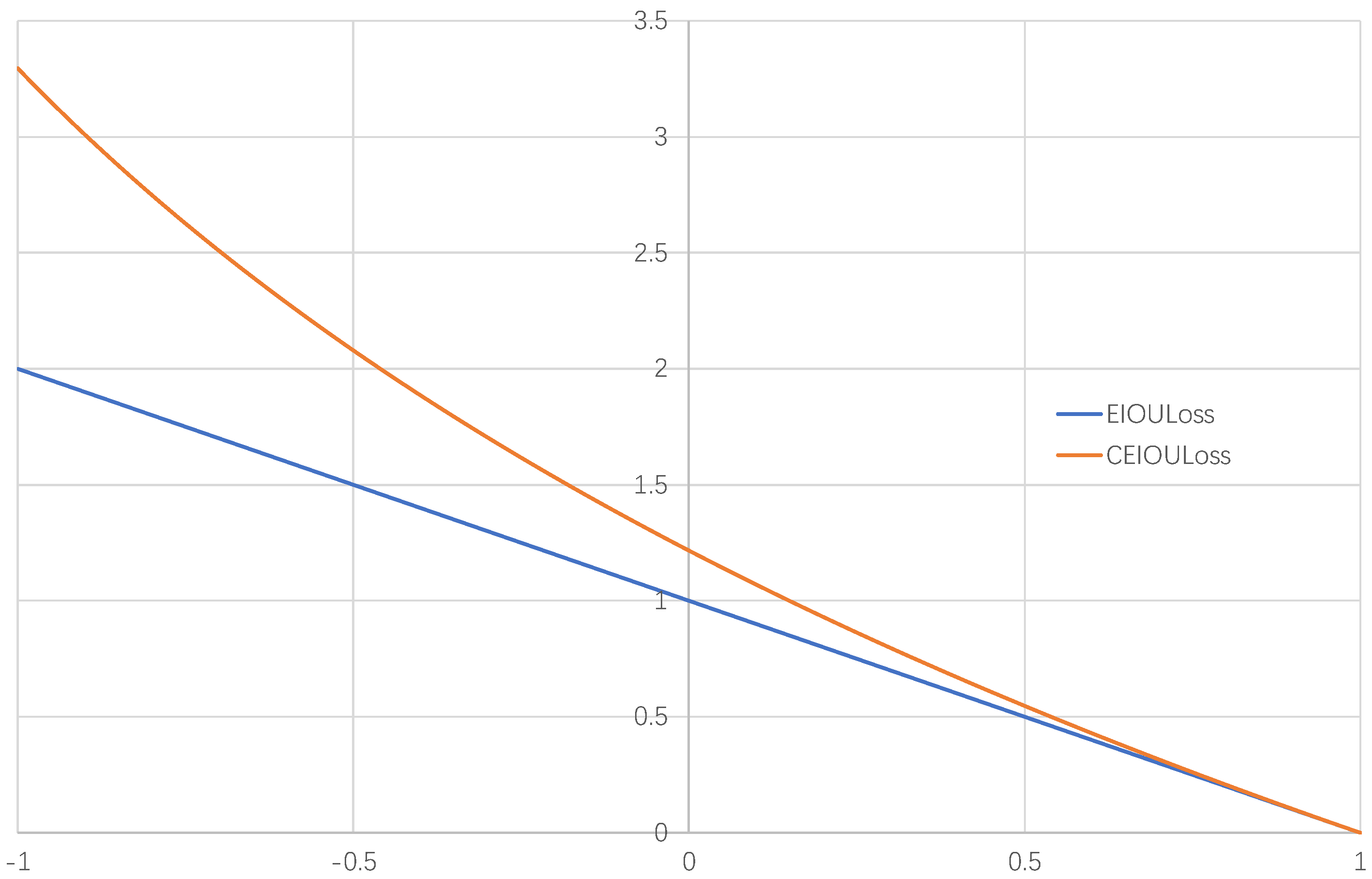
However, in the process of backpropagation, the momentum provided by for network training is constant, and it can also be understood that the gradient of is constant, which cannot give the network a larger momentum to speed up the training of the network when the predicted box and the ground truth box are too far apart. Therefore, this paper proposes a new loss function based on EIOU, namely (Curve ).
is represented by Equation (6).
The comparison of
and
is shown in
Figure 6.
It can be seen from the
Figure 6 that
is a straight line,
is a curve and both lines decrease with the increase in EIOU, but when the EIOU is small, that is, when the gap between the predicted box and the ground truth box is large,
will provide a greater momentum to the training of the network, so that next time the network adjusts the prediction box more accurately, reducing the number of times that the predicted box and the ground truth box overlap, and Since
is a straight line, the momentum it provides is equal regardless of how the magnitude of EIOU changes.
4. Results
The environment configuration for this experiment is as follows.
CPU: AMD R7-4800H; RAM: 16G; GPU: Nvidia GeForce RTX 2060 6G; Operating system: Microsoft windows 10; GPU accelerated library: CUDA 11.5 And CUDNN 11.1; Deep learning environment: Tensorflow-gpu 1.14.0 And Keras 2.2.5; IDE: Pycharm; Development language: Python 3.6.
4.1. Experimental Evaluation Criteria
In this paper, mAP50 is used as the evaluation criteria of this experiment. mAP50 is the average value of AP50 value of all classification detection results. AP50 value refers to the closed area of the precision and recall curve when the IOU threshold is 0.5. The calculation formulas of precision, recall, AP50 and mAP50 are shown as Equations (7)–(10).
TP (True Positives) represents the number of targets actually detected in this dataset, FP (False Positives) represents the number of targets detected incorrectly by the model, and FN (False Negatives) represents the number of targets missed by the model during detection.
4.2. Training Process
The training of YOLOv4 uses the idea of transfer learning. Transfer learning refers to the transfer of a model after a large number of datasets and iterative training in a known field to a target field with similar characteristics. Using this pre-trained weight can enable the network model to quickly obtain feature information in new feature fields, reducing the requirements for the number of datasets and training time during network training to a certain extent, and accelerating the network convergence speed.
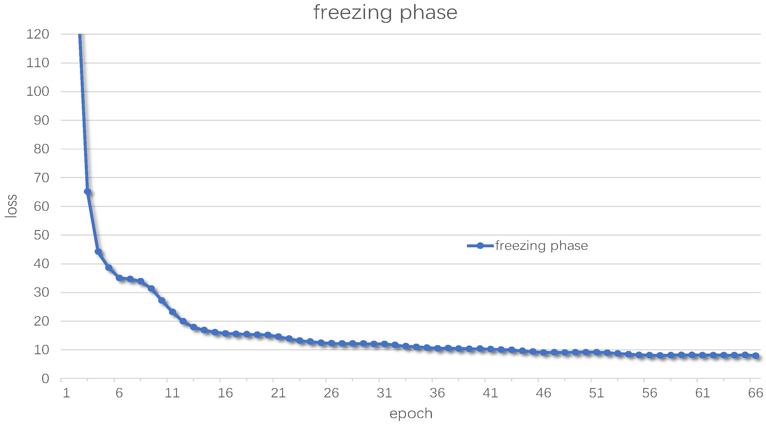
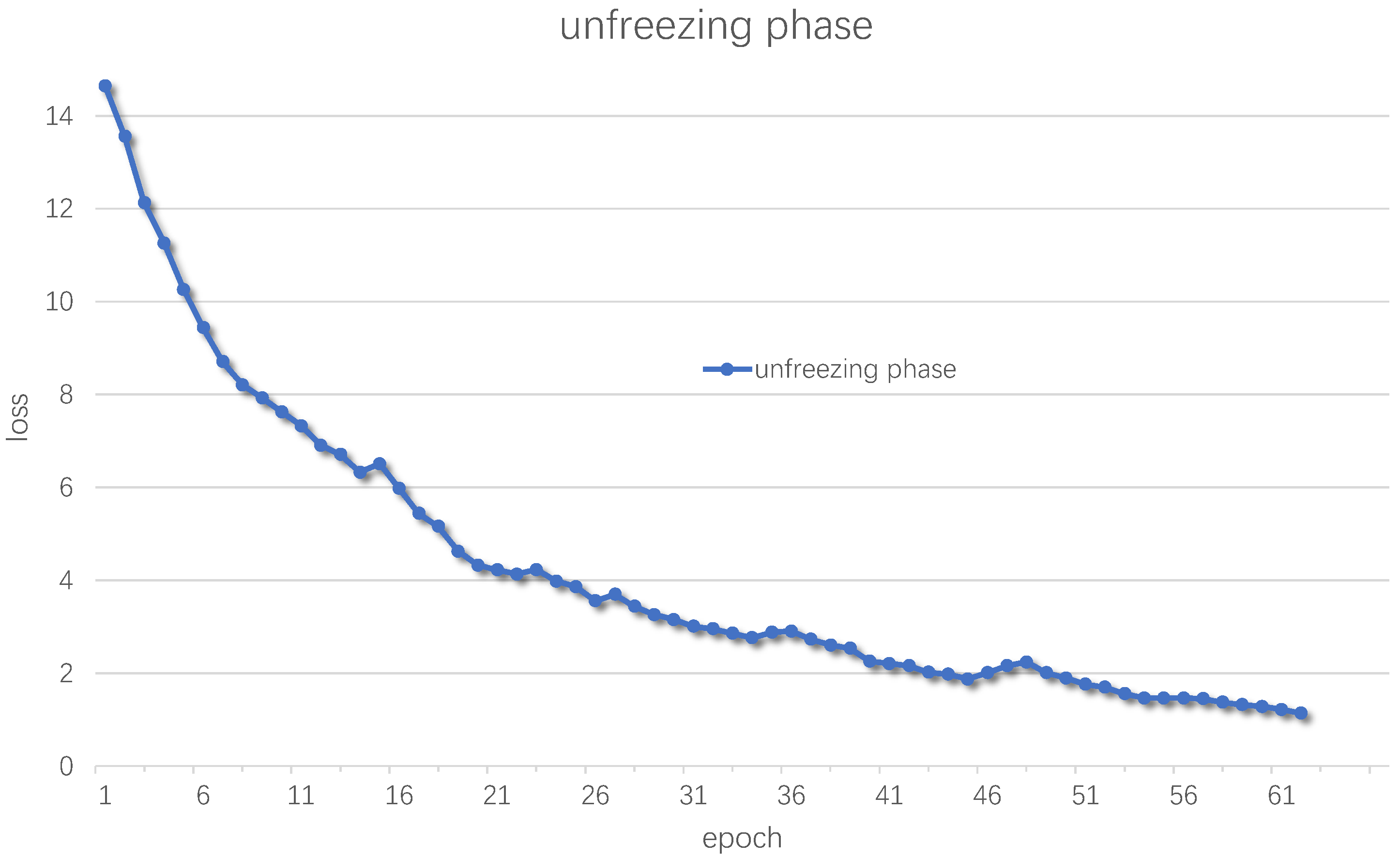
Therefore, this paper will use the already trained YOLOv4 pre-training weights for transfer training. First, the training in the freezing stage is performed, the parameters of the backbone part of the YOLO network will not change with training, and the rest of the parameters will be fine-tuned with training to adapt the network to the new dataset and speed up the initial learning speed of the network for the dataset. Set the batch size to 16, epoch to 100, and use the early stop mechanism, that is, if the loss value drops below the threshold for multiple consecutive epochs, the training in the freezing phase will be stopped. The learning rate is set to , and the cosine annealing learning rate is added, a larger learning rate will decrease at a slower rate. Then in the middle, the learning rate will decrease faster, and finally the learning rate will decrease slowly, making the training of the network more stable. In the unfreezing phase, the backbone of the network will be unfrozen, and all the parameters of the network will participate in the training and will be changed accordingly according to the dataset. Set batch size to 2, epoch to 100, and learning rate to , and the rest are the same as the freezing phase.
The change in loss value in freezing phase is shown in
Figure 7 and unfreezing phase is shown in
Figure 8.
4.3. Experiment Results
In order to further test the performance of the improved algorithm in this paper, three sets of comparative experiments will be conducted, and each set of comparative experiments will use the same training set and test set, the same training strategy and the same evaluation criteria to ensure the validity of the test results. The first set of experiments compares the improved YOLOv4 algorithm proposed in this paper with the current mainstream object detection algorithms such as YOLOv4, YOLOv3, Faster RCNN, etc. The experiment result is shown in
Table 2.
The second set of experiments is to use the same dataset to compare the improved algorithm proposed in this paper with the improved algorithms for tiny targets which are proposed in other articles, and conduct comparative experiments specifically for tiny targets. The experiment result is shown in
Table 3.
The third group of experiments is to verify the impact of the improved modules proposed in this paper on the detection of fabric defects, and to evaluate the improvement effects of each module, respectively. The experiment result is shown in
Table 4.
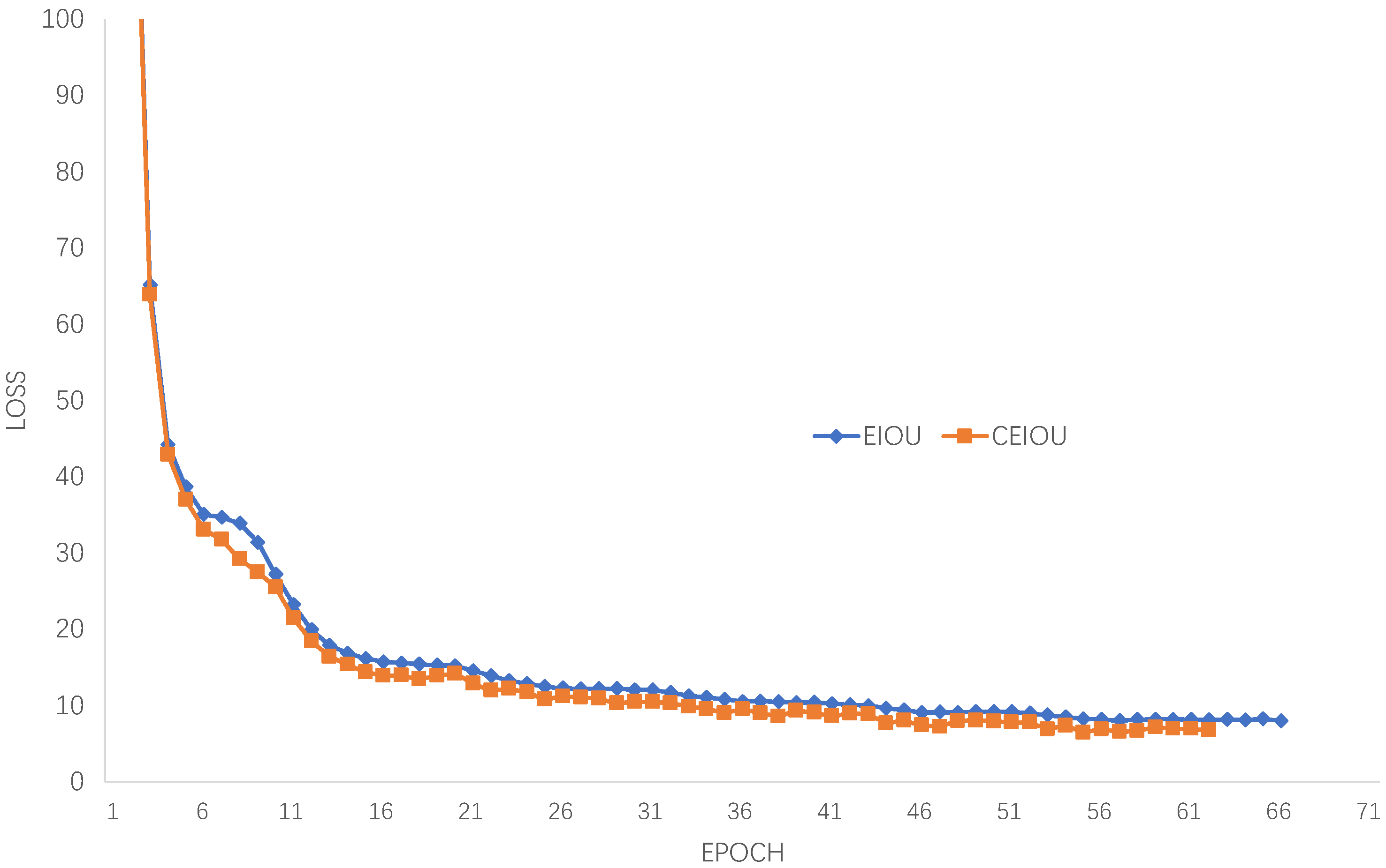
In the third set of experiments, in order to verify the optimization effect of CEIOU loss in the training phase, EIOU and CEIOU were used to train the same dataset with the same training parameters in the frozen training phase. The obtained loss value comparison chart is shown in
Figure 9.
6. Conclusions
Aiming at the insufficiency of the existing target detection algorithms for detecting small and medium-sized targets in fabric defects, a novel YOLOv4 object detection algorithm based on a series of improvements has been proposed, including the use of new data enhancement to expand the dataset, and the use of clustering algorithms to construct new yolo_anchors, adding a feature output layer for yolo_head to predict tiny targets, adding an attention mechanism so that the network will focus on high-weight areas and a new loss function to speed up the convergence of the model. In the comparative experiments with other improved networks for tiny targets, the overall mAP has increased by about 3 percentage points, and the mAP of tiny target detection has increased significantly, which is enough to reflect the effectiveness of this algorithm in tiny target detection.
With the support of hardware facilities in the future, a larger dataset and number of iterations can be used to enhance the detection ability of the network. The structure of the network can be further optimized to improve the detection ability of the network for regular size defects, as well as the use of an anchor-free method to reduce calculations while predicting and obtaining prediction boxes more accurately, or to make the network more easily transplanted into simple devices and mobile terminals to achieve faster and real-time detection.


