Assessment and Prediction of Extreme Temperature Indices in the North China Plain by CMIP6 Climate Model

Abstract

Extreme temperature events are becoming more frequent due to global warming, and have critical effects on natural ecosystems, social and economic spheres, human production and life. Predicting changes in temperature extremes and trends under future climate scenarios helps to assess the impact of climate change accurately. Based on climate observations from 54 meteorological stations in the North China Plain and the projection data from seven general circulation models (GCMs) from the Coupled Model Intercomparison Project phase 6 (CMIP6), this paper researches nine representative extreme temperature indices under four typical climate scenarios. The aim is to reveal the temporal and spatial variations in extreme temperature indices in the North China Plain during the past (1971–2010) and the future (2061–2100). The results show that: using a support vector machine (SVM) to perform regression analysis on the multi-GCMs prediction results, the root mean square error (RMSE) and relative standard deviation (RSD) of the multi-model ensemble simulations obtained by the SVM method are lower than those of the arithmetic mean method and can better match the trend of the historical extreme temperature index; the extreme high temperature index is predicted to show a significant upward trend in the future, while the extreme low temperature index will decrease significantly; and there are significant spatial differences in the extreme temperature index in both historical and future periods, with the extreme temperature index under the high radiation forcing scenario (SSP585) showing the most considerable variation and the most significant spatial differences.

1. Introduction

According to the IPCC report [1], the trend of global warming is strong, with a temperature increase rate of 0.13 °C/10a over the last 50 years. Extreme climate events (heat waves, droughts, etc.) are becoming more common and intense, wreaking havoc on human life, society, the economy, and the environment [2]. In the context of future global warming, the North China Plain, with its flat topography, abundant light and heat resources and being an essential agricultural food production base in China, will most likely be threatened by more severe extreme events in terms of economic population, agricultural production, and ecological environment. As a result, it is critical to fully consider the risk of extreme temperature changes in the North China Plain, improve the prediction of extreme temperature changes of the region, face this serious challenge together, and rationally promote the region’s and country’s green and sustainable joint development and ecological civilization.

The Global Climate Model (GCM) includes fundamental processes in circles of the climate system and can depict material and energy flow between them. It is a valuable tool for delving into the mechanisms of past climate change and forecasting future climate change. The results provide the data needed to study climate change and its effects at multiple spatial and temporal scales and a scientific foundation for human response and adaptation to future climate change [3]. In the 20 years since the CMIP was implemented, the World Climate Research Programme (WCRP) Working Group on Coupled Models (WGCM) has launched the sixth International Coupled Model Comparison Program (CMIP6), which includes the most significant number of participating models, the most abundantly designed numerical experiments, and the most considerable amount of simulated data [4]. The climate system simulations are closer to observed values [5,6]. It has been widely utilized in temperature and precipitation simulations and predictions, among other things [7]. Zhu and Yang examined CMIP6 with CMIP5 simulations of temperature and precipitation on the Qinghai–Tibet Plateau, finding that most CMIP6 models performed better than CMIP5 [8]. At the same time, You et al. also found that CMIP6 could better reproduce the climatic characteristics of China, and the cold bias was improved compared with CMIP5 [9]. Tian found that the simulated precipitation of the CMIP6 model in China was in good agreement with the observed values. In the future scenario, the average annual precipitation in China showed increased rates of precipitation and fluctuation. In northern China the increased rate of precipitation was higher than in southern China [10].

Extreme climate events will become more frequent and intense due to global warming; therefore, predicting and analyzing the occurrence and impacts of extreme climate events has become a demanding problem in climate science. Traditional mathematical methods are being used in the current scientific investigation on predicting extreme temperatures in the North China Plain. For example, Xiao et al. used a statistical downscaling method to obtain daily station-by-station data and estimate future climate change in the North China Plain under two typical climate scenarios (RCP4.5 and RCP8.5) on a multi-model ensemble by downscaling future climate scenarios from 33 GCMs in CMIP5 [11]. Machine learning is a popular study topic in artificial intelligence and pattern recognition. Its theories and methods have been applied to a broad range of issues in engineering and scientific fields. Changes in the meteorological environment have temporal and spatial diversity, and the change process is non-linear variable. Therefore, machine learning approaches can successfully analyze and predict meteorological data [12]. Dong et al. used three machine learning models (XGBoost, SVM, MARS) to estimate the amount of daily diffuse solar radiation (Rd) based on local inputs, stating that three machine learning models can estimate daily Rd based on local inputs [13]; Mo et al. investigated the potential of four machine learning (ML) models, namely, extreme Learning Machine (ELM), Genetic Programming (GP), and RNN [14]. Dong et al. presented a support vector machine (SVM) approach for predicting solar radiation. They stated that the SVM method would be a promising alternative to standard methods for evaluating solar radiation at any location [15]. This demonstrates how machine learning methods can simulate and forecast temperature data in the research domain.

In the North China Plain, there are essentially no studies on the use of machine learning algorithms for extreme temperature prediction. This study uses statistical downscaling methods to downscale the data of seven GCMs in CMIP6 in time and space. It uses Support Vector Regression (SVM) [16] to regress and analyze the simulated data of multiple climate models to obtain a relatively reasonable prediction model. In this paper, nine commonly used extreme temperature indices were selected to firstly simulate and evaluate the extreme temperature indices in the historical period of the North China Plain and then predict the spatial and temporal variability of the extreme temperature indices in the future climate scenarios of the North China Plain, to provide a scientific basis for addressing the disaster risks associated with extreme temperature events. Therefore, predicting future extreme temperature trends in the North China Plain can aid in understanding the extreme climate risks that global warming may bring to agricultural production, allowing agricultural production levels to be stabilized and regional food security to be ensured [7,17].

2. Materials and Methods

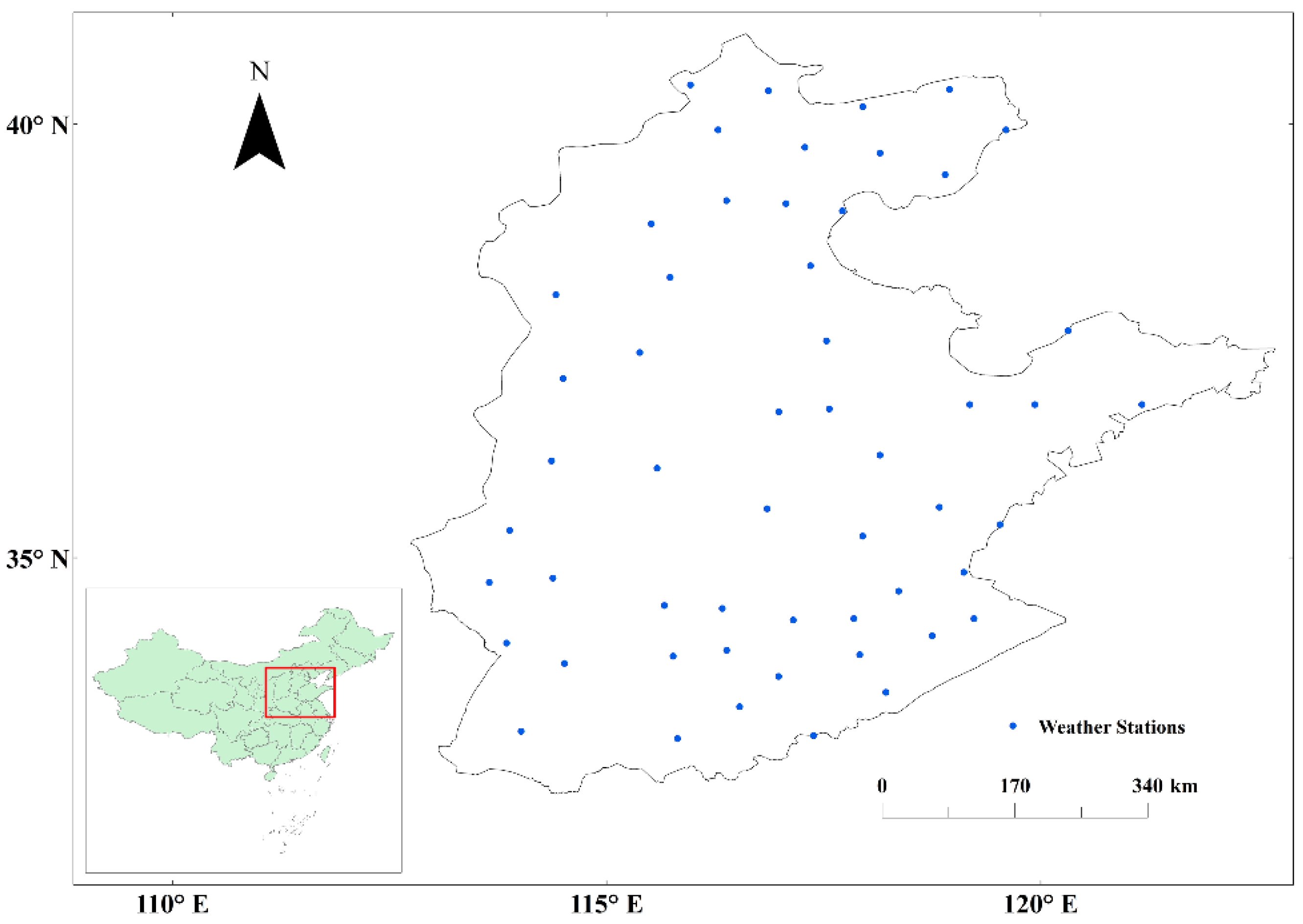
2.1. Overview of the Study Area

The North China Plain spans seven provinces and cities in Beijing: Tianjin, Hebei, Lu, Henan, Anhui, and Suzhou, covering about 300,000 km². It reaches the Yanshan Mountains in the north, leans against the Taihang Mountains in the west, borders the Bohai Sea and the Yellow Sea in the east, and is bounded in the south by the mainstream of the Huai River and the northern Jiangsu irrigation canal. The North China Plain is flat and has a warm temperate monsoon climate with simultaneous rain and heat, suitable for crop growth and an important food production area in China [6]. At the same time, the eastern part belongs to the sea–land transition zone, and the southern part is a climate transition zone with complex climatic conditions, which is an area prone to extreme weather events [16].

2.2. Data Sources

The daily temperature observations at 54 meteorological stations (Figure 1) in the study area were derived from the China Meteorological Science Data Service Sharing Network’s (https://data.cma.cn/, accessed on 1 January 2022) monthly surface precipitation and temperature value grid point dataset (V2.0), which includes four major climate factors: maximum temperature, minimum temperature, total solar radiation, and rainfall. The dataset is based on a 0.5 × 0.5° horizontal resolution spatial interpolation of data from more than 2400 ground stations throughout China [18].

The model data are the historical climate simulation and future scenario experimental data from the CMIP6 climate model. The future scenario experimental data are a combination of different representative concentration pathways (RCPs) and shared socioeconomic pathways (SSPs) [19]. RCPs are a series of enrichment and comprehensive emissions scenario [20] of a 21st century under the influence of human activities on climate change prediction model input parameters, to describe the future population, social economy, science and technology, energy consumption and land use change, greenhouse gases, reactant gas and aerosol emissions, as well as the concentration of the atmospheric composition. CMIP6 not only upgrades RCP2.6, RCP4.5, RCP6.0, and RCP8.5 to SSP126, SSP245, SSP460, and SSP585, but it also provides more options for scientists in future climate prediction. The new emission modes also include SSP119, SSP434, SSP534OS, and SSP370. CMIP6 is used in many models, and seven models were chosen for this investigation from the historical and future scenario data releases (https://esgf-node.llnl.gov/search/cmip6, accessed on 1 January 2022), with model characteristics provided in

Table 1. Information of the 7 global climate models (GCMs) applied in the study.

ID	GCM Name	GCM Abbreviations	The Developer	COUNTRY/AREA
1	BCC-CSM2-MR	BCC	BCC	China
2	CanESM5	CAN	CCCMA	Canada
3	CNRM-CM6-1	CNR1	CNRM	France
4	CNRM-ESM2-1	CNR2	CNRM	France
5	IPSL-CM6A-LR	IPS	IPSL	France
6	MIROC6	MIR1	MIROC	Japan
7	MRI-ESM2-0	MRI	MRI	Japan

. The following four typical climate scenarios were chosen for this study, representing four climatic pathways of (1) sustainable development, (2) moderate development, (3) local development, and (4) conventional development, based on the representativeness of future climate scenarios and the completeness of data under the corresponding climate scenarios:

• SSP126 is a scenario with a stable radiative forcing of 2.6 W/m² in 2100 [21];
• SSP245 is a medium forcing scenario, and the radiative forcing is stabilized at 4.5 W/m² in 2100;
• SSP370 is a net radiative forcing scenario with a stable radiative forcing of 7.0 W/m² in 2100, which represents a mixture of high social vulnerability and relatively high perceived radiative forcing [22];
• SSP585 achieves a strong forcing scenario in 2100, with an anthropogenic radiative forcing of 8.5 W/m².

The selected month-by-month raster data of seven GCMs are downscaled temporally and spatially in this work to obtain daily site data. The Wagga Wagga Institute of Agriculture in Australia developed a statistical downscaling method [11,23] that can effectively downscale the output of GCMs to a fine spatial and temporal scale to enhance the prediction of future extreme temperature events. Unlike many other statistical downscaling methods requiring data regarding atmospheric circulation or sea surface temperature as predictors, it contains spatial and temporal downscaling components. The approach can generate daily data series in real-time from monthly gridded GCMs. Compared to dynamic downscaling, it can adjust for biases in GCM data and is computationally efficient enough to be applied to many GCMs. As a result, the approach can be used to investigate future climate change uncertainty.

2.3. Extreme Temperature Indices

In this study, nine extreme temperature indices defined by the Expert Team on Climate Change Detection and Indices (ETCCDI) (http://etccdi.pacificclimate.org, accessed on 2 January 2022) were selected (

Table 2. Name and interpretation of the nine extreme temperature indices.

ID	Descriptive Name	Definition
TXx	Hottest day	Highest TX (°C)
TNx	Hottest night	Highest TN (°C)
DTR	Diurnal temperature range	Average difference between TX and TN (°C)
TXn	Coldest day	Lowest TX (°C)
TNn	Coldest night	Lowest TN (°C)
TX90p	Warm days	Number of days when TX > 90th percentile (d)
TN90p	Warm nights	Number of days when TN > 90th percentile (d)
SU	Summer days	Number of days with TX > 25 °C (d)
FD	Frost days	Number of days with TN < 0 °C (d)

), and all of the indices were closely related to extreme temperature. The monthly maximum value of daily maximum temperature (TXx), monthly maximum value of daily minimum temperature (TNx), monthly minimum value of daily maximum temperature (TXn), number of summer days (SU), and number of frost days (FD). The remaining indices are percentages, such as the number of warm night days (TN90p) and the number of warm day days (TX90p). They are calculated based on the number of days with temperatures above or below the 90th or 10th percentile for each climate model at each location. Using the 1961–2000 reference period, percentages were calculated relative to the year, centered on a 5-day window for each calendar day [24]. The daily temperature range (DTR) is calculated as the difference between the maximum and minimum temperatures to measure extreme temperature variability. Every metric was calculated as an annual value. The extreme temperature index was calculated using the R package “climdex.pcic”.

2.4. The Support Vector Machine

The SVM data mining method is a data mining method based on statistical learning theory that can successfully deal with many problems, such as regression problems (time-series analysis) and pattern recognition (classification problems, discriminant analysis), and can be extended to fields and disciplines such as prediction and comprehensive analysis. It is based on Vapnik et al.’s [25] statistical learning theory, Mercer’s kernel expansion theorem, and the results of contemporary optimization methods. The best solution is found by translating the sample space to a multi-dimensional feature space and reducing the optimum regression hyperplane issue to a quadratic convex programming problem with constraints in the feature space. Due to the convex nature of the optimality issue, the SVM model, in contrast to regularly used neural network models, provides a unique solution [26].

The regression problem, understood mathematically, is given a training sample $D=\left\{\right(x_1,y_1),(x_2,y_2),\dots ,(x_m,y_m)\}, y_i\in R:x_i \in R$ by learning to hopefully fit each sample point as closely as possible to a linear model of the shape $f\left(\mathit{x}\right)={\mathsf{\omega }}^{\mathrm{T}}\mathit{x}+\mathit{b}\left(\mathsf{\omega }\in \mathit{R}, \mathit{b}\in \mathit{R}\right)$ so that $f\left(\mathit{x}\right)$ and y are as close as possible, where $x$ is the input vector, referred to as the influence factor, $y_i$ is the predicted object, and $w$ and $b$ are the model parameters to be determined. In traditional regression models for samples $\left(\mathit{x}, \mathit{y}\right)$, the model usually calculates the loss directly based on the difference between the model output $f(\mathit{x}$) and the true output $y$, and the loss is zero when $f\left(\mathit{x}\right)$ is exactly the same as $y$. In support vector regression, it is assumed that the maximum error with $\epsilon$ is allowed between $f\left(\mathit{x}\right)$ and y, and the loss is calculated only when the absolute value of difference between $f\left(\mathit{x}\right)$ and y is greater than $\epsilon$. In other words, with $f\left(\mathit{x}\right)$ as the center, an interval band with a width of 2$\epsilon$ is constructed. If the training sample falls into this interval band, the prediction is considered correct. Thus, the SVR problem can be formalized as in Equation (1):

$$\begin{array}{c}\min \\ \omega ,b\end{array}\frac{{\Vert \omega \Vert }^2}{2}+C{\displaystyle {{\displaystyle \sum }}_{i=1}^m}{l}_{\epsilon }\left(f\right(x_i)-y_i)$$

(1)

where $C$ is the regularization constant, and $l_{\epsilon }$ is the loss function.

If a given sample is not linearly regressed when using support vector machines to solve regression problems [27], the sample can be mapped from the original space to a multi-dimensional feature space. Then, the sample can be a linear regression in the multi-dimensional feature space, and then an appropriate regression hyperplane can be found. That is, the sum-fitting regression function $f\left(\mathit{x}\right)={\mathsf{\omega }}^{\mathrm{T}}\mathsf{\phi }\left(\mathit{x}\right)+\mathit{b}$, where $\mathsf{\phi }\left(\mathit{x}\right)$ represents the feature vectors that $\mathsf{\phi }\left(\mathit{x}\right)$ maps to the sample $\mathit{x}$. Finally, the optimal regression function can be used for regression prediction. The regression model based on SVM uses the principle of structured risk minimization to minimize the risk of training experience, reduce the complexity of the model, and improve the generalization ability of the model.

Furthermore, this work compares the SVM and arithmetic mean calculation outcomes utilizing Root Mean Square Error (RMSE) and relative standard deviation (RSD) based on the root mean square error (RMSE) between model simulation and observation, with the formula

$$RMSE=\sqrt{{{\displaystyle \sum }}_{i=1}^n{\left(x_i-y_i\right)}^2/n}$$

(2)

$$RSD=\sqrt{{{\displaystyle \sum }}_{i=1}^n{\left(x_i-\overline{x}\right)}^2/\left(n-1\right)}/\overline{x}\times 100\%$$

(3)

where $x_i$, $y_i$ are the simulated and observed values in year $i$, respectively, and $\overline{x}$ is the arithmetic mean.

3. Results

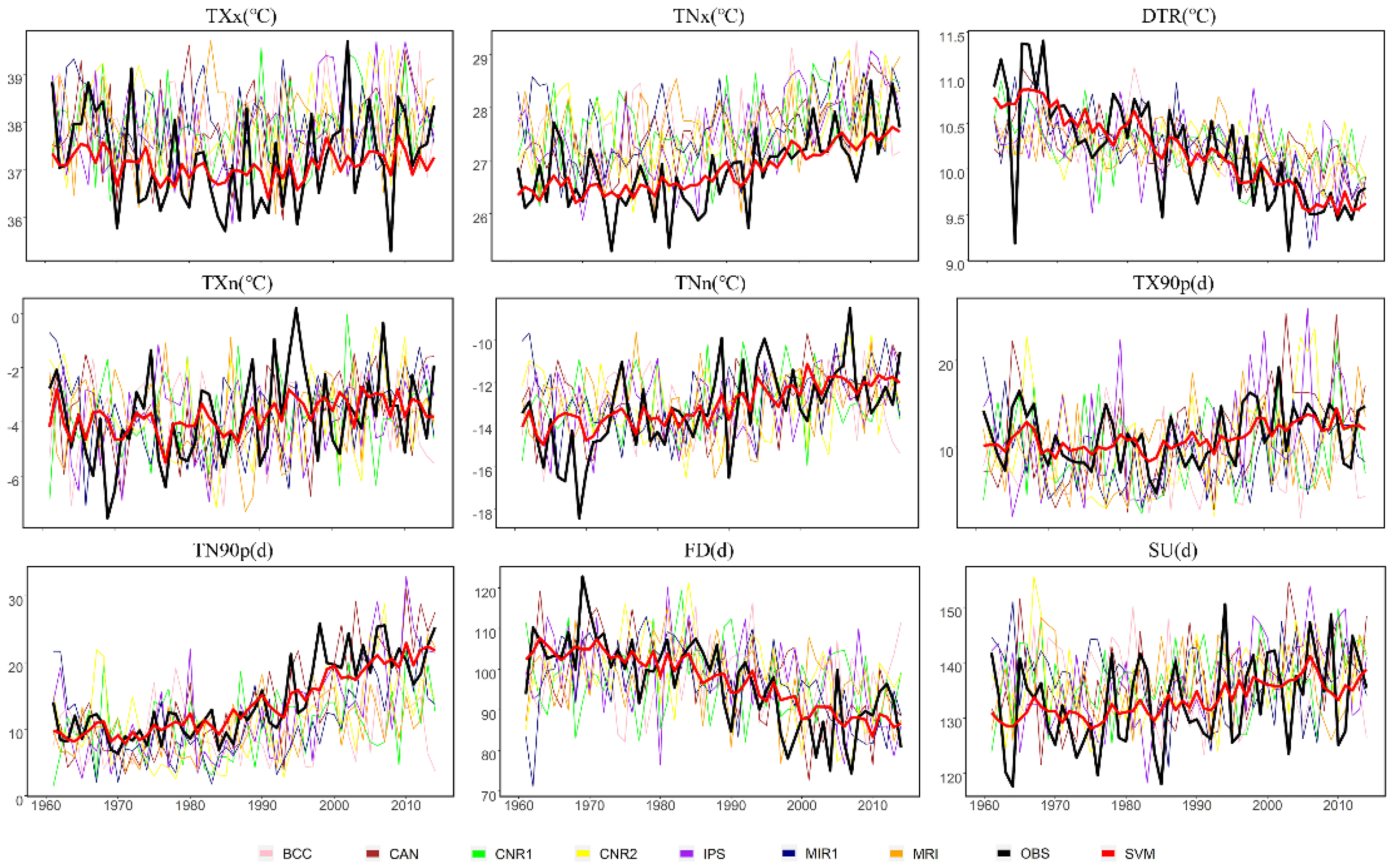
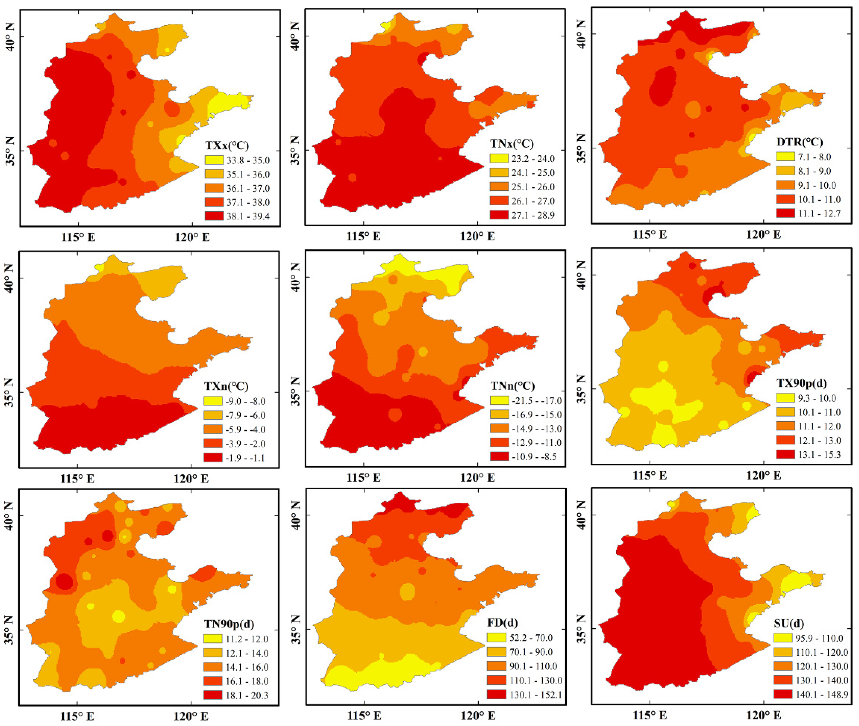
3.1. Simulation and Assessment of Extreme Temperature Indices in the North China Plain during the Historical Period

All seven extreme high temperature indices (TXx, TNx, TXn, TNn, TN90p, TX90p, and SU) showed a fluctuating upward trend during this period, while the extreme low temperature indices (FD) and DTR showed a fluctuating downward trend, as shown by the trend of simulated and observed extreme temperature indices (OBS) in the North China Plain from 1961 to 2014 (Figure 2). The calculated temperature indices of the model simulations did not precisely match the actual values, and the extreme temperature indices of the SVM simulated values were all quite similar to the observed index fluctuations over time. The RMSEs and RSDs between the nine extreme temperature indices simulated by the seven climate models and the multi-model arithmetic average (MEAN) and actual values are much bigger than the simulated values by the SVM, as shown in

Table 3. Root mean square error (RMSE) and relative standard deviation (RSD) between simulations and observed values for the nine extreme temperature indices.

GCMs	TXx	TNx	DTR	TXn	TNn	TX90p	TN90p	FD	SU
BCC	2.00 (5.38%)	1.67 (6.24%)	0.68 (6.68%)	2.31 (79.64%)	2.94 (22.81%)	6.60 (58.43)	8.66 (60.55%)	15.35 (17.28%)	13.88 (11.11%)
CAN	2.03 (5.47%)	1.58 (5.89%)	0.73 (7.23%)	2.46 (86.65%)	2.88 (22.46%)	6.62 (58.83%)	7.03 (50.02%)	13.31 (14.89%)	14.27 (11.30%)
CNR1	2.05 (5.53%)	1.62 (6.05%)	0.76 (7.45%)	2.68 (96.35%)	3.18 (25.02%)	6.55 (58.14%)	8.59 (60.00%)	16.07 (18.20%)	14.03 (11.11%)
CNR2	1.91 (5.16%)	1.59 (5.94%)	0.77 (7.58%)	2.63 (90.56%)	3.23 (25.16%)	6.17 (55.00%)	7.73 (54.33%)	14.13 (15.88%)	13.00 (10.34%)
IPS	2.06 (5.55%)	1.57 (5.87%)	0.75 (7.43%)	2.66 (92.95%)	3.10 (24.16%)	7.02 (62.47%)	7.60 (53.72%)	14.89 (16.66%)	13.63 (10.86%)
MIR1	2.04 (5.48%)	1.63 (6.08%)	0.72 (7.12%)	2.46 (87.00%)	3.06 (23.91%)	6.53 (57.94%)	7.91 (55.41%)	14.13 (15.85%)	14.73 (11.74%)
MRI	2.14 (5.75%)	1.66 (6.19%)	0.73 (7.19%)	2.65 (91.11%)	3.16 (24.61%)	6.66 (59.33%)	7.69 (53.61%)	14.08 (15.97%)	13.46 (10.62%)
MEAN	1.75 (4.72%)	1.41 (5.25%)	0.66 (6.48%)	2.12 (73.32%)	2.68 (21.00%)	4.31 (38.18%)	5.88 (40.93%)	11.55 (12.94%)	11.44 (9.08%)
SVM	1.38 (3.71%)	0.90 (3.36%)	0.54 (5.33%)	1.76 (60.45%)	2.30 (17.96%)	3.66 (32.63%)	4.27 (30.12%)	9.48 (10.61%)	9.17 (7.27%)

. The simulated results of the SVM, as shown in Figure 2 and

Table 4. Trends in nine extreme temperature indices in the North China Plain from 1961 to 2014.

GCMs	TXx (°C/10a)	TNx (°C/10a)	DTR (°C/10a)	TXn (°C/10a)	TNn (°C/10a)	TX90p (d/10a)	TN90p (d/10a)	FD (d/10a)	SU (d/10a)
BCC	−0.03	0.07	−0.12	0.02	0.04	−0.26	0.80	−0.52	−0.62
CAN	0.10	0.30	−0.12	0.29	0.43	1.67	3.82	−3.64	1.93
CNR1	0.04	0.16	−0.09	0.09	0.17	0.18	1.05	−0.79	0.91
CNR2	0.10	0.18	−0.04	0.03	0.08	1.11	1.65	−1.83	1.40
IPS	0.16	0.30	−0.09	0.12	0.28	1.24	2.77	−2.55	2.13
MIR1	−0.11	0.10	−0.19	0.16	0.28	−0.13	1.57	−2.45	−1.03
MRI	0.04	0.13	−0.09	0.02	0.14	0.53	1.47	−1.55	0.31
MEAN	0.04	0.18	−0.10	0.10	0.20	0.62	1.88	−1.90	0.72
OBS	0.01	0.24	−0.27	0.30	0.70	0.45	2.92	−4.76	1.66
SVM	0.01	0.23	−0.26	0.19	0.51	0.57	2.73	−4.16	1.62

, have reduced uncertainty in interannual variability and can better reverse the temporal patterns of the extreme temperature indices. The simulated values correlate well with the observed values, making them helpful in assessing and forecasting extreme temperature events in the North China Plain.

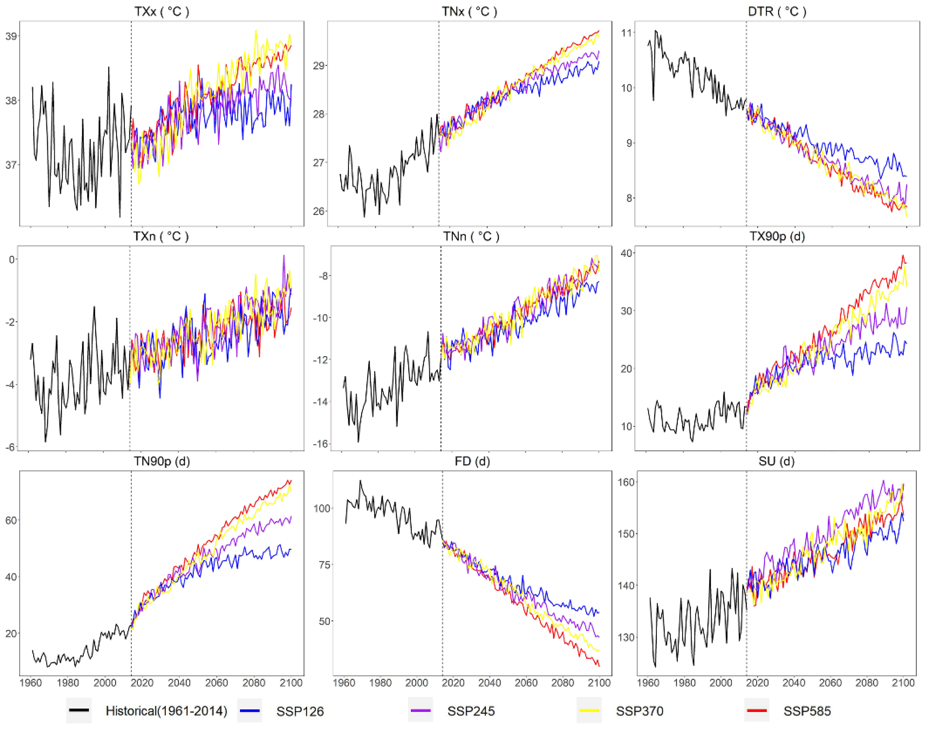
3.2. Temporal Variability Characteristics of Extreme Climate Index Changes under Future Climate Scenarios

The extreme high temperature index (TXx, TNx, TXn, TNn, TN90p, TX90p, and SU) increases significantly under the four climate scenarios (SSP126, SSP245, SSP370, and SSP585) over the projection period (2015–2100) (Figure 3). In contrast, the extreme low temperature index (TXx, TNx, TXn, TNn, TN90p, TX90p, and SU) decreases significantly (FD). Extreme temperature indices show similar trends in all four climate scenarios through 2050. Except for TXn, TNn, and Su, the differences in extreme temperature indices change rates under different climate scenarios steadily rise after 2050. The extreme temperature indices TXx, TNx, TX90p, and TN90p climb the quickest under the SSP585 climate scenario; for example, TX90p will be close to 40 d in 2100, whereas the rise is flatter and stabilizes under the SSP126 climate scenario; for instance, TX90p will be approximately 24.3 d in 2100. Under several climate scenarios, the change rates of the intense heat indices TXn, TNn, and Su did not differ much, and all exhibited a strong upward trend. The extreme low temperature index (FD) drops the fastest under the SSP585 climate scenario, dropping 15.5 days between 2080 and 2100. In contrast, I drop slowly and stabilize the SSP126 climate scenario, falling just 4.2 days between 2080 and 2100. With a reduction of roughly 1.2 °C, the temperature steadily rises.

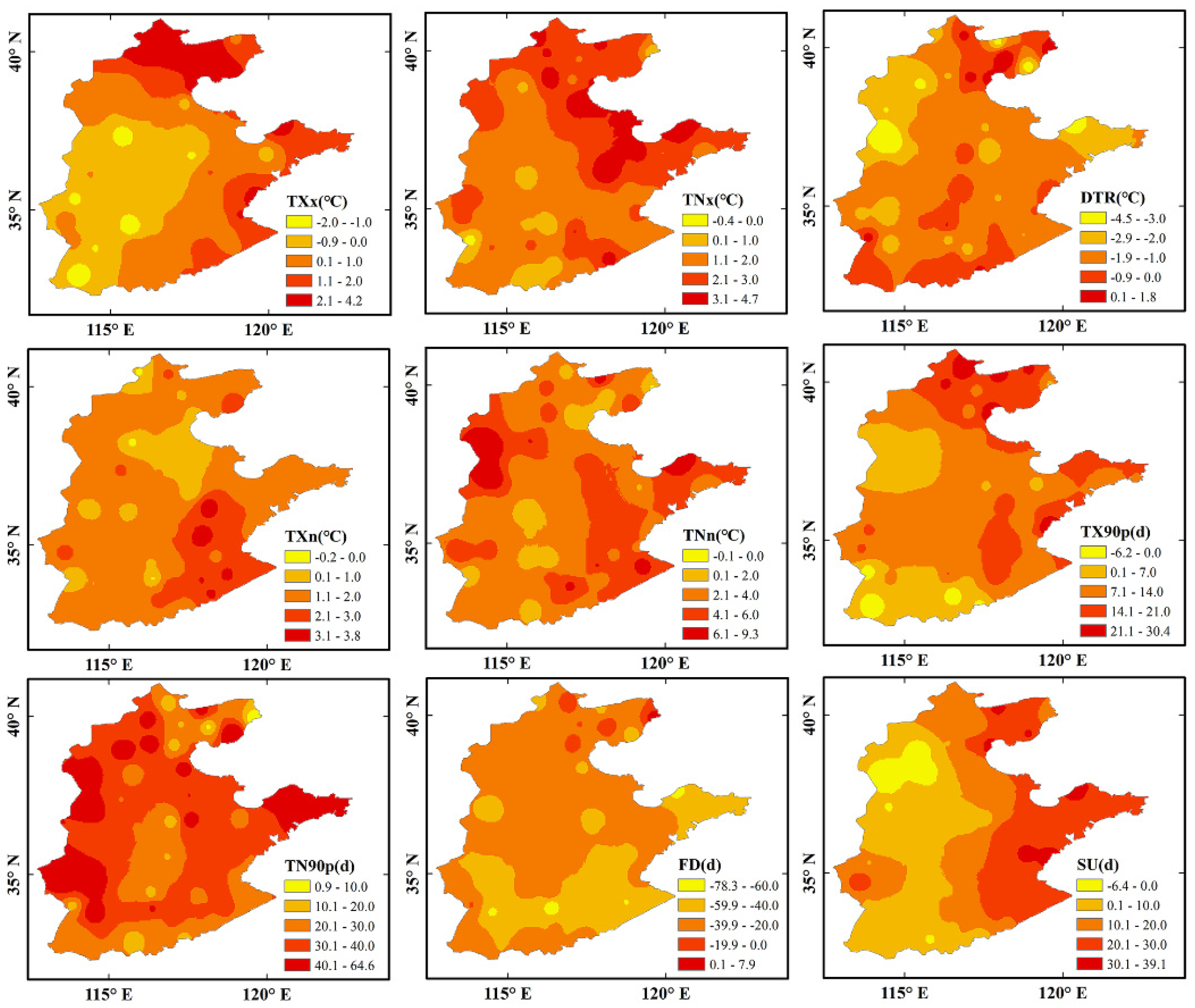
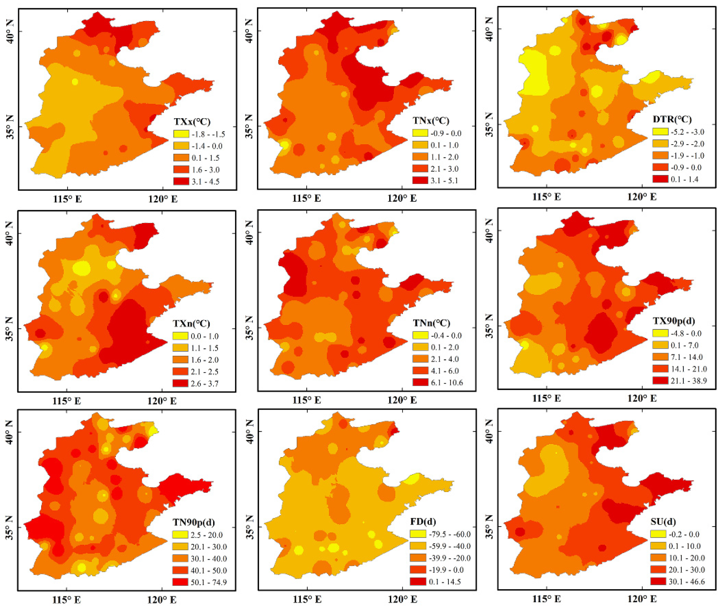
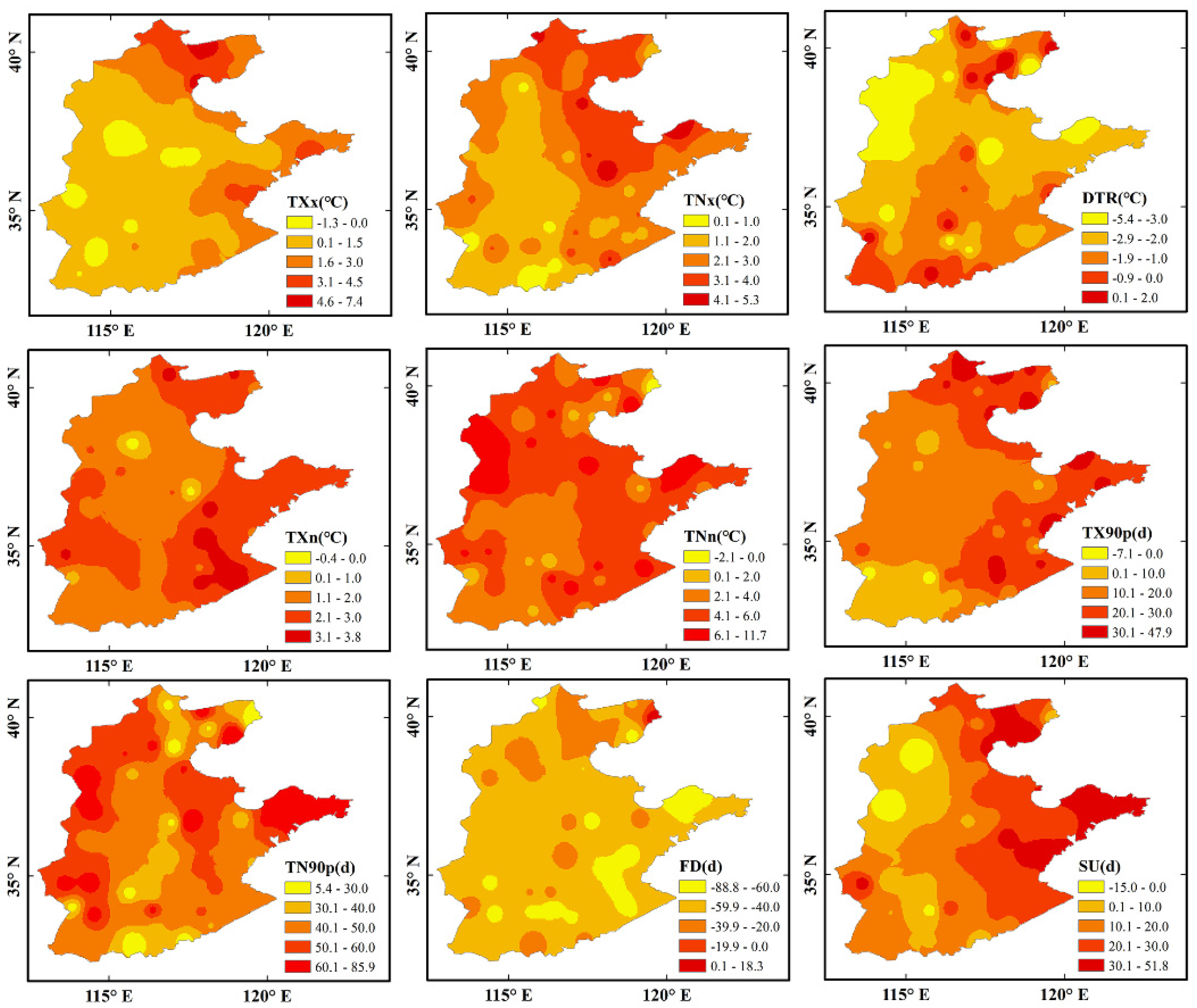
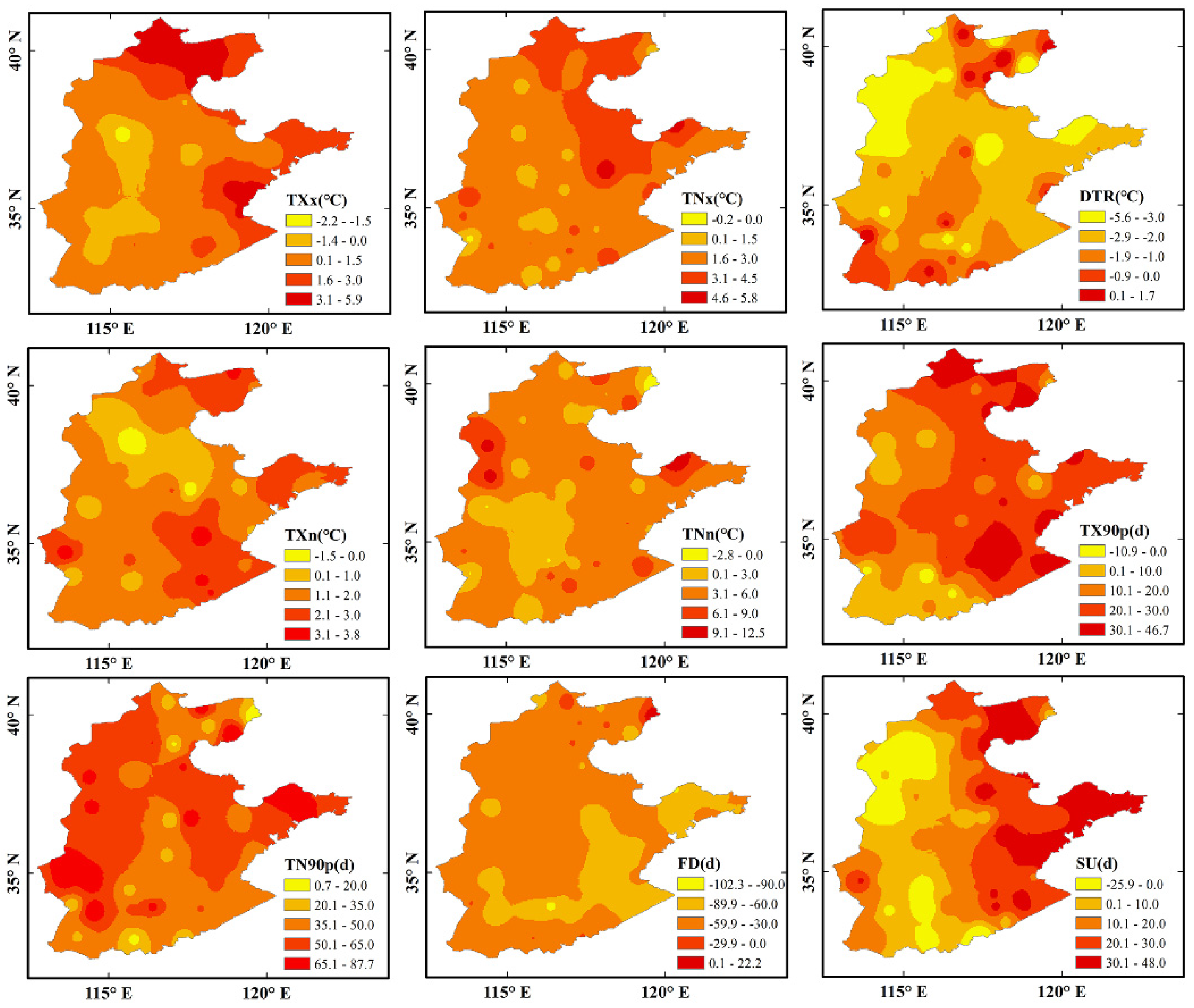
3.3. Spatial Variation Characteristics of Extreme Temperature Indices in the North China Plain

There are evident geographical disparities in the extreme temperature indices in the North China Plain throughout the reference period (1971–2010) due to changes in the geographic position, terrain, biological environment, and other variables (Figure 4). tx90p and tn90p have relatively significant differences between the north and south; TNx, TXn, and TNn have the opposite spatial distribution characteristics of DTR, being high in the south and low in the north, with north–south differences between 6.7 and 13 °C; TXx and TNx have relatively large differences between the north and south; and FD has significant north–south variances: for example, FD in the southern region is typically less than 90 days, and even less than 70 days in specific locations, but FD in the northern part is often greater than 90 days.

Figure 5, Figure 6, Figure 7 and Figure 8 exhibit the regional variation features of extreme temperature indices under four future climatic scenarios (2061–2100). TXx increased by more than 1.1 °C in the northern and southern parts of the North China Plain compared to the base period, while most of the central regions decreased by 0~0.9 °C; TNx, TXn, TNn, TX90p, TN90p, and SU all showed an overall increasing trend, but there were some differences between the southern and northern parts; the extreme low temperature index FD showed a decreasing trend in most areas of the North China Plain, with decreases ranging The geographic variability of the extreme temperature indices in the SSP245, SSP370, and SSP585 climate scenarios are similar to that in the SSP126 scenario. However, it is more extensive, notably in the SSP585 high forcing climate scenario (Figure 6, Figure 7 and Figure 8). The increase in TXx under the SSP585 climate scenario was more significant than 1.6 °C in the southern and northern parts of the North China Plain and between 0.1 and 1.5 °C in most of the central area (Figure 8); the variability of other extreme temperature indices was more significant than under the SSP126 climate scenario, and spatial differences were more prominent.

4. Discussion

Similar to comparative studies [11], we simulated and predicted the spatial and temporal variation characteristics of extreme temperature indices in the North China Plain for different periods of history and the future using SVM regression using day-by-day temperature monitoring data from 54 meteorological stations and CMIP6 climate model data processed by statistical downscaling. Based on the CMIP5 global climate model, Bai et al. [2] simulated and predicted the climate of the North China Plain. The results showed that the maximum and minimum temperature increases under both climate scenarios (RCP4.5 and RCP8.5) were similar until 2040. The temperature increase under RCP8.5 was much higher than that under RCP4.5 after 2040. The extreme temperature index in the study area was studied by Wang et al. [28] using the independent weighted mean method based on the CMIP6 climate model. The results showed that the extreme high temperature index tends to increase in the future. In contrast, the extreme low temperature index decreases, and the extreme temperature index under the high radiative forcing scenario (SSP585) has the most significant change. The findings of this study indicate a similar trend, with the four climatic scenarios showing relative changes in the extreme climate index before 2050, and more evident disparities in the changes after 2050, with SSP585 showing the highest evolution and SSP126 leading the slightest difference. However, the comparative forecast findings still contain some discrepancies due to climate model selection and simulation methodology variances. The results of Bai and Wang et al., for example, demonstrate that from 2040, the growth in different climatic scenarios will be more diverse. In contrast, the estimated threshold of this study is 2050. As a result, further research may be carried out by adding or filtering climate models for comparison studies. Meanwhile, while the SVM method is more effective in the simulation and evaluation of extreme temperature indices in the historical period than individual climate models and the arithmetic mean, other machine learning algorithms, such as random forests and decision trees, must be compared to it to find a more suitable simulation algorithm for this study area.

Although the simulation method of GCMs in CMIP6 has improved noticeably, there are still some uncertainties in the corresponding future GHG emissions due to variances in the feedback processes of various GCMs, which has a significant impact on the predictability of the findings [20,29]. Furthermore, due to substantial differences in structural principles, climate forcing settings, emission scenario design, and model resolution, the simulation performance of climate change can be significantly different among GCMs. The simulation results may have a bias, which increases the difficulty of future climate simulation and the uncertainty of simulation results. To address these problems, the simulation effect of the CMIP6 climate model can be improved.

The first is the downscaling approach, divided into two categories: statistical downscaling and dynamic downscaling. Statistical downscaling establishes a functional relationship between global-scale meteorological factors and regional-scale meteorological factors to obtain more reasonable simulation results, whereas active downscaling nests the regional climate model in the global climate model to receive high-resolution regional climate information [30,31]. The downscaling approach efficiently solves the problem of climate model scale mismatch by converting the output of large-scale, low-resolution GCMs or regional climate models into small-scale, high-resolution regional climatic information. By layering the regional climate model RegCM4.0 into the global climate model in one direction, Hao Lisheng et al. [32] increased the simulation accuracy of the climate in the Hebei area. Chen Hao et al. [33] used an artificial neural network-based statistical downscaling model to estimate evaporation from the Yarkant River basin and reservoirs under future climate change scenarios, reducing the uncertainty of simulation findings.

The second technique is a multi-model ensemble simulation. The use of a multi-model ensemble simulation can reduce the uncertainty of climate model simulation results and improve the simulation capability of climate models due to the differences in the selection, resolution, parameterization, and response processes of physical parameters among climate models. The GCM simulation of global and regional climate has certain uncertainties due to differences in the selection, resolution, parameterization, and response processes of physical parameters among climate models, and the use of multi-model ensemble simulation can reduce the uncertainty of climate model simulation results and improve the simulation capability of climate models. Chen et al. [34] conducted a study on predicting future changes in precipitation in China based on ensemble-averaged simulation results of 16 climate models with equal weight coefficients. The simulation results better reproduced the climatic state distribution characteristics of annual rainfall at the regional scale in China. Through climate model simulations, Hu et al. [35] discovered that equal-weight ensemble simulations outperformed median ensemble simulations. The multi-model ensemble simulation approach does not imply that the primary averaging method is utilized alone to create the model ensemble, and the simulation capabilities of various climate change models vary. The simulation ability of the model ensemble can be effectively improved by using the weighted averaging method instead of the equal-weighted averaging method and assigning different weighting coefficients to other climate models, which is also an important future development direction for using climate models to study climate change [36].

5. Conclusions

In this paper, we use a statistical downscaling of data from seven GCMs, then SVM was used to stimulate and predict the future climate of the North China Plain under various climate scenarios using a multi-GCM model ensemble, analyze its spatial and temporal variability characteristics, and provide the necessary database for future climate adaptation and response to climate change.

(1)

The simulated values of extreme temperature indices from the multi-climate model SVM method better agree with the observed values than individual GCM models. The arithmetic means method is suitable for simulating and predicting extreme temperature indices in the North China Plain.

(2)

The extreme high temperature indices (TXx, TNx, TXn, TNn, TN90p, TX90p, and SU) indicate a considerable growing tendency for the four future climate scenarios (2061–2100), whereas the extreme low temperature indices drop dramatically. TXx, TNx, TN90p, and TX90p altered the most in the SSP585 climate scenario, whereas TXx, TNx, TN90p, and TX90p changed the least with the SSP126 climate scenario. Under different climate scenarios, TXn, TNn, and Su did not alter appreciably.

(3)

In the North China Plain, there are significant spatial differences in extreme temperature indices in both historical and future periods, except DTR. The variance in the extreme temperature index grows with the growth of the scenario’s radiative forcing, and spatial differences become more pronounced, reaching a maximum under the SSP585 climate scenario.

References

1. Stocker, T.F.; Qin, D.; Plattner, G.; Tignor, M.M.; Allen, S.K.; Boschung, J.; Nauels, A.; Xia, Y.; Bex, V.; Midgley, P.M.; et al. Climate Change 2013. The Physical Science Basis. In Working Group I Contribution to the Fifth Assessment Report of the Intergovernmental Panel on Climate Change; Cambridge University Press: Cambridge, UK, 2014. [Google Scholar]
2. Bai, H.; Xiao, D.; Liu, J.; Wang, H.; Zhang, H.; Li, Z. Spatio-temporal pattern of extreme climate events and agro-meteorological disasters in North China from 1965 to 2014. Geogr. Geoinform. Sci. 2018, 34, 99–105. [Google Scholar]
3. Zhao, Y.; Xiao, D.; Bai, H. Prediction and application of CMIP5 climate model for future climate change in China. Meteorol. Sci. Technol. 2019, 47, 608–621. [Google Scholar]
4. Zhou, T.; Zou, L.; Chen, X. Review of the Sixth International Comparative Program of Coupled Models (CMIP6). Prog. Clim. Chang. Res. 2019, 87, 5–16. [Google Scholar]
5. Fu, Y.; Lin, Z.; Guo, D. Improvement of the simulation of the summer East Asian westerly jet from CMIP5 to CMIP6. Atmos. Ocean. Sci. Lett. 2020, 13, 550–558. [Google Scholar] [CrossRef] [Green Version]
6. Kim, Y.H.; Min, S.K.; Zhang, X.; Sillmann, J.; Sandstad, M. Evaluation of the CMIP6 multi-model ensemble for climate extreme indices. Weather. Clim. Extrem. 2020, 29, 100269. [Google Scholar] [CrossRef]
7. Chen, H.P.; Sun, J.Q. Robustness of Precipitation Projections in China: Comparison between CMIP5 and CMIP3 Models. Atmos. Ocean. Sci. Lett. Engl. Ed. 2014, 7, 67–73. [Google Scholar]
8. Yyzab, C.; Syab, C. Evaluation of CMIP6 for historical temperature and precipitation over the Tibetan Plateau and its comparison with CMIP5. Adv. Clim. Chang. Res. 2020, 11, 239–251. [Google Scholar]
9. You, Q.; Cai, Z.; Wu, F.; Jiang, Z.; Pepin, N.; Shen, S.S. Temperature dataset of CMIP6 models over China: Evaluation, trend and uncertainty. Clim. Dyn. 2021, 57, 17–35. [Google Scholar] [CrossRef]
10. Tian, D.; Guo, Y.; Dong, W. Future Changes and Uncertainties in Temperature and Precipitation over China Based on CMIP5 Models. Adv. Atmos. Sci. Engl. 2015, 32, 10. [Google Scholar] [CrossRef]
11. Xiao, D.; Zhao, Y.; Bai, H.; Tang, J.; Feng, P.; Liu, D. Modeling and estimation of climate in the North China Plain by cmip5 global climate model. Geogr. Geo-Inf. Sci. 2020, 36, 8. [Google Scholar]
12. Yu, S. Analysis and prediction model of meteorological environment and winter heating energy consumption of hospitals based on machine learning. China Equip. Eng. 2021, 27–28. [Google Scholar]
13. Dong, J.; Wu, L.; Liu, X.; Fan, C.; Leng, M.; Yang, Q. Simulation of Daily Diffuse Solar Radiation Based on Three Machine Learning Models. Comput. Model. Eng. Sci. 2020, 123, 49–73. [Google Scholar] [CrossRef]
14. Chen, J.L.; Li, G.S.; Xiao, B.B.; Wen, Z.F.; Lv, M.Q.; Chen, C.D.; Jiang, Y.; Wang, X.X.; Wu, S.J. Assessing the transferability of support vector machine model for estimation of global solar radiation from air temperature. Energy Convers. Manag. 2015, 89, 318–329. [Google Scholar] [CrossRef]
15. Chen, J.L.; Li, G.S. Evaluation of Support Vector Machine for Estimation of Solar Radiation from Measured Meteorological Variables; Springer: Vienna, Austria, 2014. [Google Scholar]
16. Chapelle, O.; Haffner, P.; Vapnik, V.N. Support Vector Machines for Histogram-Based Image Classification. IEEE Trans. Neural Netw. 1999, 10, 1055–1064. [Google Scholar] [CrossRef] [PubMed]
17. Elguindi, N.; Grundstein, A.; Bernardes, S.; Turuncoglu, U.; Feddema, J. Assessment of CMIP5 global model simulations and climate change projections for the 21st century using a modified Thornthwaite climate classification. Clim. Chang. 2014, 122, 523–538. [Google Scholar] [CrossRef]
18. Zhao, Y.; Zhu, J.; Xu, Y. Establishment and quality assessment of precipitation grid data set in China in recent 50a. Meteorol. Sci. 2014, 34, 414–420. [Google Scholar]
19. Taylor, K.E.; Stouffer, R.J.; Meehl, G.A. An Overview of CMIP5 and the Experiment Design. Bull. Am. Meteorol. Soc. 2012, 93, 485–498. [Google Scholar] [CrossRef] [Green Version]
20. Moss, R.H.; Edmonds, J.A.; Hibbard, K.A.; Manning, M.R.; Rose, S.K.; Van Vuuren, D.P.; Carter, T.R.; Emori, S.; Kainuma, M.; Kram, T. The next generation of scenarios for climate change research and assessment. Nature 2010, 463, 747–756. [Google Scholar] [CrossRef]
21. Zhang, L.; Chen, X.; Xin, X. Overview and review of THE CMIP6 Scenario Model Comparison Plan (Scenari-oMIP). Prog. Clim. Chang. Res. 2019, 15, 519–525. [Google Scholar]
22. Tebaldi, C.; Debeire, K.; Eyring, V.; Fischer, E.; Fyfe, J.; Friedlingstein, P.; Knutti, R.; Lowe, J.; O’Neill, B.; Sanderson, B.; et al. Climate model projections from the Scenario Model Intercomparison Project (ScenarioMIP) of CMIP6. Earth Syst. Dyn. 2021, 12, 253–293. [Google Scholar] [CrossRef]
23. Liu, D.L.; Zuo, H. Statistical downscaling of daily climate variables for climate change impact assessment over New South Wales, Australia. Clim. Chang. 2012, 115, 629–666. [Google Scholar] [CrossRef]
24. Zhi, L.; Zheng, F.L.; Liu, W.Z.; Jiang, D.J. Spatially downscaling GCMs outputs to project changes in extreme precipitation and temperature events on the Loess Plateau of China during the 21st Century. Glob. Planet. Chang. 2012, 82–83, 65–73. [Google Scholar]
25. Cortes, C. Support-Vector Networks. Mach. Learn. 1995, 20, 273–297. [Google Scholar] [CrossRef]
26. Chen, L. Improving Least Squares Support Vector Machine and Its Application; East China Jiaotong University: Nanchang, China, 2014. [Google Scholar]
27. Su, Y.X.; Xu, H.; Yan, L.J. Support Vector Machine-Based Open Crop Model (SBOCM): Case of Rice Production in China. Saudi J. Biol. Sci. 2017, 24, 537–547. [Google Scholar] [CrossRef]
28. Wang, H.; Xiao, D.; Zhao, Y.; Bai, H.; Zhang, K.; Tang, J.; Liu, J.; Guo, F.; Liu, D. Evaluation and prediction of extreme temperature index in North China Plain based on CMIP6 climate model. Geogr. Geoinform. Sci. 2021, 37, 86–94, 142. [Google Scholar]
29. Zhou, T.; Chen, X. Uncertainty problems of climate sensitivity, climate feedback process and 2 °C warming threshold value. Acta Meteorol. Sin. 2015, 73, 624–634. [Google Scholar]
30. Cheng, A.; Feng, Q.; Zhang, J.; Li, Z.; Wang, G. A review on the response process of climate change under future climate scenarios. Geogr. Sci. 2015, 35, 84–90. [Google Scholar]
31. Fowler, H.J.; Blenkinsop, S.; Tebaldi, C. Linking Climate Change Modelling to Impacts Studies: Recent Advances in Downscaling Techniques for Hydrological Modelling; Wiley-Blackwell: Hoboken, NJ, USA, 2007. [Google Scholar]
32. Hao, L.; Xiang, L.; Zhang, J. Test analysis of China’s climate change projection data in Hebei Province. J. Atmos. Sci. 2015, 38, 362–370. [Google Scholar]
33. Chen, H.; Yang, T.; Hu, G.; Wang, S. Analysis of evaporation change of reservoir in Yeerqiang Basin under climate change. People’s Yangtze River 2016, 47, 31–34. [Google Scholar]
34. Chen, L. Prediction of CMIP5 model on the change of extreme precipitation events in China at the end of the 21st century. Sci. Bull. 2013, 58, 743–752. [Google Scholar]
35. Hu, Q.; Jiang, D.; Fan, G. Assessment of the ability of CMIP5 global climate model to simulate climate on the Tibetan Plateau. Atmos. Sci. 2014, 38, 924–938. [Google Scholar]
36. Xu, Y.; Gao, X.; Giorgi, F. Upgrades to the reliability ensemble averaging method for producing probabilistic climate-change projections. Clim. Res. 2010, 41, 61–81. [Google Scholar] [CrossRef] [Green Version]
Figure 1. Spatial distribution of meteorological stations in the study area.
Applsci 12 07201 g001
Figure 2. Trends in observed and simulated nine extreme temperature indices in the North China Plain from 1961 to 2014.
Applsci 12 07201 g002
Figure 3. Trends in nine extreme temperature indices in the North China Plain under four future climate scenarios.
Applsci 12 07201 g003
Figure 4. Spatial characteristics of extreme temperature indices in the North China Plain from 1971 to 2010.
Applsci 12 07201 g004
Figure 5. Spatial characteristics of changes in extreme temperature indices in the North China Plain from 2061 to 2100 under the SSP126 scenario.
Applsci 12 07201 g005
Figure 6. Spatial characteristics of changes in extreme temperature indices in the North China Plain from 2061 to 2100 under the SSP245 scenario.
Applsci 12 07201 g006
Figure 7. Spatial characteristics of changes in extreme temperature indices in the North China Plain from 2061 to 2100 under the SSP370 scenario.
Applsci 12 07201 g007
Figure 8. Spatial characteristics of changes in extreme temperature indices in the North China Plain from 2061 to 2100 under the SSP585 scenario.
Applsci 12 07201 g008