Article

Unsteady Aerodynamic Characteristics of a High-Speed Train Induced by the Sudden Change of Windbreak Wall Structure: A Case Study of the Xinjiang Railway

1
National Rail Transit Electrification and Automation Engineering Technology Research Center (Hong Kong Branch), Hong Kong, China
2
Department of Civil and Environmental Engineering, The Hong Kong Polytechnic University, Hung Hom, Kowloon, Hong Kong, China
3
Key Laboratory of Traffic Safety on Track of Ministry of Education, School of Traffic & Transportation Engineering, Central South University, Changsha 410075, China
4
Department of Civil and Environmental Engineering, The Hong Kong University of Science and Technolgy, Clear Water Bay, Kowloon, Hong Kong, China
*
Authors to whom correspondence should be addressed.
Appl. Sci. 2022, 12(14), 7217; https://doi.org/10.3390/app12147217
Submission received: 24 June 2022 / Revised: 15 July 2022 / Accepted: 15 July 2022 / Published: 18 July 2022
(This article belongs to the Special Issue Aerodynamics of High-Speed Trains)

Abstract

:
Under strong winds, the effect of sudden windbreak transition (WT) on high-speed trains is severe, leading to a deterioration of train aerodynamics and sudden yawing motion of the car body. To address these problems, based on a high-speed train and the specific geometric conditions derived from Xinjiang railway, first, the impact of a WT on the train and reasons for sudden changes in aerodynamic forces were determined by flow structural analysis. Furthermore, based on a multibody system dynamic model, the dynamic responses to WT were analysed. The results show that the impacts of WT were the strongest on the head car. WT had a strong effect on the train due to the unreasonable structural shape and the insufficient height of the windbreak in the transition region. This led to a strong push effect on the train; subsequently, the train’s dynamic characteristics deteriorated.

1. Introduction

In strong wind areas, crosswinds are a typical safety risk for train operation, and train aerodynamics are important to consider [1,2,3]. High-speed trains are affected by various factors, including the nose and head shape, the car body shape, the pantograph, and the train speed [4]. Furthermore, wind speed is a key factor that been studied using prescribed yaw angles for various train speeds [5]. Various methods are applied to study train aerodynamics under crosswinds. Generally, full-scale tests can directly reflect the aerodynamic performance of a train [6,7]. In the United Kingdom, Gallagher et al. [8] compared the aerodynamic performances of trains using the CFD method, model testing, and full-scale tests under crosswinds. Due to the limitations of full-scale tests, such as the high cost and experimental settings, model tests are typically conducted, which include the wind tunnel and moving model tests [9,10]. Various wind tunnel tests have been conducted with crosswinds, including studies of current and new train designs [11], investigation of the geometric details on train aerodynamics [12], etc. Pressure is easily measured with moving model tests, but aerodynamic forces are not easy to measure directly. Therefore, Xiang et al. [13] and Liu et al. [14] developed a method for examination of the aerodynamic force characteristics of moving vehicles under crosswinds. With a focus on train stability under crosswinds, Dorigatti et al. [15] compared static and moving experimental results for a model passenger train and found that there were small differences in the pressure distributions that were limited to the nose and underbody of the train. With advancements in computational efficiency, an increasing number of studies on train aerodynamics have been conducted using the CFD method [16], including studies on the effect of bogie’s geometric complexity on force measurement, the slipstream of freight trains and passenger trains under crosswinds [17,18], and the prediction performance of different turbulence models for train aerodynamics under crosswinds.
Terrain and facilities surrounding the railway, including cuttings, embankments, bridges, and tunnels, affect trains in the presence of crosswinds [19,20]. Owing to varying terrain, transition regions can be generated beside the railway. Under a crosswind, these transitions lead to an unsteady wind. Using a wind tunnel test, Zhang et al. [21] built a 1:20 scale model in an attempt to study train aerodynamics in the transition region between the subgrade and tunnel under crosswinds. The results of their study demonstrated that the impact of the transition from the cutting to the tunnel was greater than that of the embankment–tunnel transition. The effects of long-span bridge towers on a train were investigated by Li et al. [22] and Wu et al. [23] using wind tunnel tests. The results demonstrated that due to the shielding effects of towers, sudden wind load changes considerably affect train aerodynamics. In addition, the findings indicated that the corresponding dynamic responses of the train fluctuated considerably.
Windbreak walls are built to protect the running safety of trains under crosswinds due to their low cost and their effectiveness [24,25]. Uniform and regular windbreaks result in a significant improvement in train safety in general; however, when the windbreak is built on varying terrain, windbreak transitions (WTs) occur along the railway. Sudden and irregular WTs affect a train’s aerodynamic and dynamic performances [26]. For instance, a windbreak wall was built along the LanXin high-speed railway in China [27,28]; however, some portions of this railway pass through complex landforms, which include flat ground, embankments, and cuttings. Therefore, the windbreak was built discontinuously, creating many irregular transition areas between different types of terrain, as shown in Figure 1. Full-scale tests were conducted, which showed that when trains passed through WT areas under crosswinds, a yawing phenomenon occurred. This results in potential effects on passenger comfort and operational safety.
According to practice cases, as shown in Figure 1, the focus of the present study was WT structure shape. We first analysed transient aerodynamic forces, followed by investigation of the flow field deterioration mechanism in this WT. Furthermore, the dynamic running state of the train was evaluated.

2. Materials and Methods

2.1. Objective Geometry

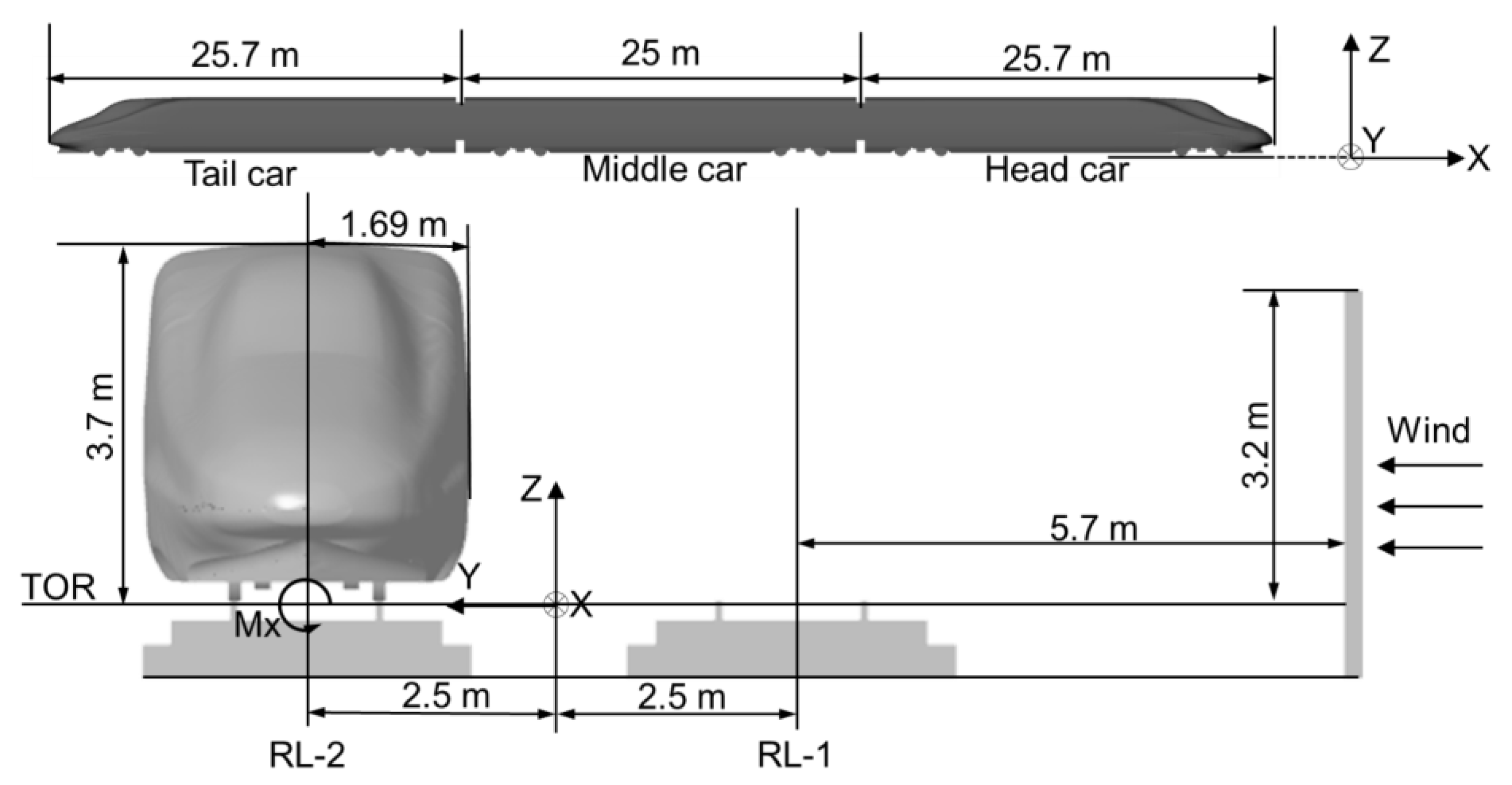
The WT was studied based on a model of the characteristics of the actual railway; detailed shapes and sizes are shown in Figure 2. In practice, the distance from the windbreak to the centre of the railway is differs between flat ground cutting positions; therefore, there is a right-angle connection structure between these two windbreaks. In practice, the windbreak is modularly constructed, with a fixed length of 5 m, resulting in a height difference between the two continuous modules. In the computational model studied in this work, the windward side (WWS) boundary is 60 m from the centre of the double railway lines, and the leeward side (LWS) boundary is 80 m from the same position. According to the actual conditions, the train speed is 250 km/h, and the wind speed is 35 m/s, with a 90° wind angle. China’s high-speed train, CRH 2, was considered in this study, as shown in Figure 3. The train height, h, was used as the reference size in the following analyses.
Generally, the length of a high-speed train is longer than three cars, according to Niu et al. [29]; with the length of the train increased from one car to four cars under crosswinds, the head car’s side force reaches maximum and changes slightly with changes in length. However, the tail car’s side force decreases as the length of the train increases. The windproof ability is worse in the WT region, and the wind impacts the train suddenly. As the length increases, the changing law of the aerodynamic force of the train is the same as that reported by Niu et al. [29]. Therefore, in terms of the most dangerous car—i.e., the head car—a length of three cars is sufficient. The aerodynamic forces of the tail car are higher with the present length than those with a longer train, so qualitative analysis can be conducted, reflecting the actual situation to some extent. In previous studies [30,31], sudden aerodynamic forces were also researched for train three cars; therefore, in this paper, we investigated a case involving three cars.

2.2. Research Method

Based on decomposed sliding mesh technology [32], and to better meet the requirements of numerical methods for grid size, a scale model (1/10) was utilized for calculation and analysis. Because the moving state was studied in the current work and under crosswinds, there is an unsteady flow around the train, so a turbulence model should be used. Although large eddy simulation (LES) and detached eddy simulation (DES) can show more detailed flow structures, they require considerable computational resources and are time-consuming and costly. However, for research on engineering applications, the unsteady Reynolds-averaged Navier–Stokes (URANS) method is also feasible for reliable aerodynamic forces and average flow fields [33]. In previous studies [34,35], the URANS method and different turbulence models were used for similar research geometry, such as shear stress transport (SST) k-ω turbulence models, renormalisation group (RNG) k-ε turbulence, the realisable k-ε turbulence model, etc. Not only does the SST k-ω method save computational cost, but it also has a higher predicting ability with respect to forces and the flow field around the train [36,37]. Therefore, a URANS method based on the SST k-ω method [38] was used in the present study. The time step was set to 0.0001 s to make the Courant–Friedrichs–Lewy (CFL) less than 1 in most cells around the train. Simulations were conducted using Fluent 18.1, which is based on the finite volume method (FVM), to discretise the governing equations. A second-order upwind scheme was set for the convection and diffusion terms, and a second-order implicit scheme was set for the time derivative. The pressure–velocity coupling and solution procedures were based on the Semi-Implicit Method for Pressure-Linked Equations Consistent (SIMPLEC) algorithm.
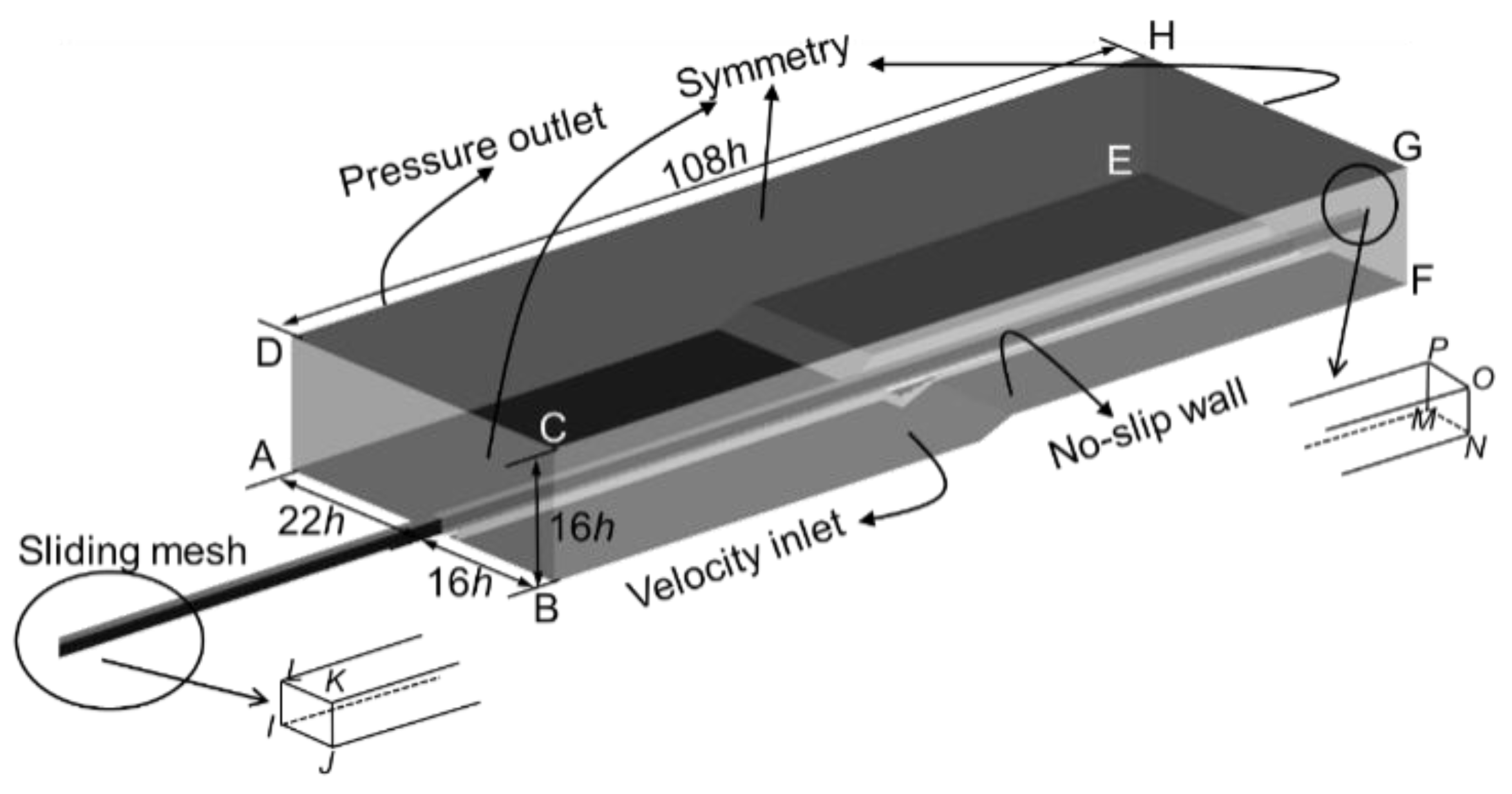
The size of the computational domain and corresponding boundary conditions are illustrated in Figure 4. For the fixed domain, symmetry wall boundary conditions were set for the faces of ABCD, EFGH, and DCGH, with no convective flux across a symmetry plane; therefore, the normal velocity component at the symmetry plane is zero. To reproduce the crosswind effect, a velocity-inlet boundary condition was used on the BFGC face. In addition, a zero-pressure outlet was set for the AEHD face to simulate the real atmospheric environment. Finally, no-slip walls were used for the ground, windbreak, and train surfaces. In the sliding zone, the IJKL and MNOP faces were zero-pressure outlets, and the other faces were interface boundary conditions.

2.3. Computational Mesh

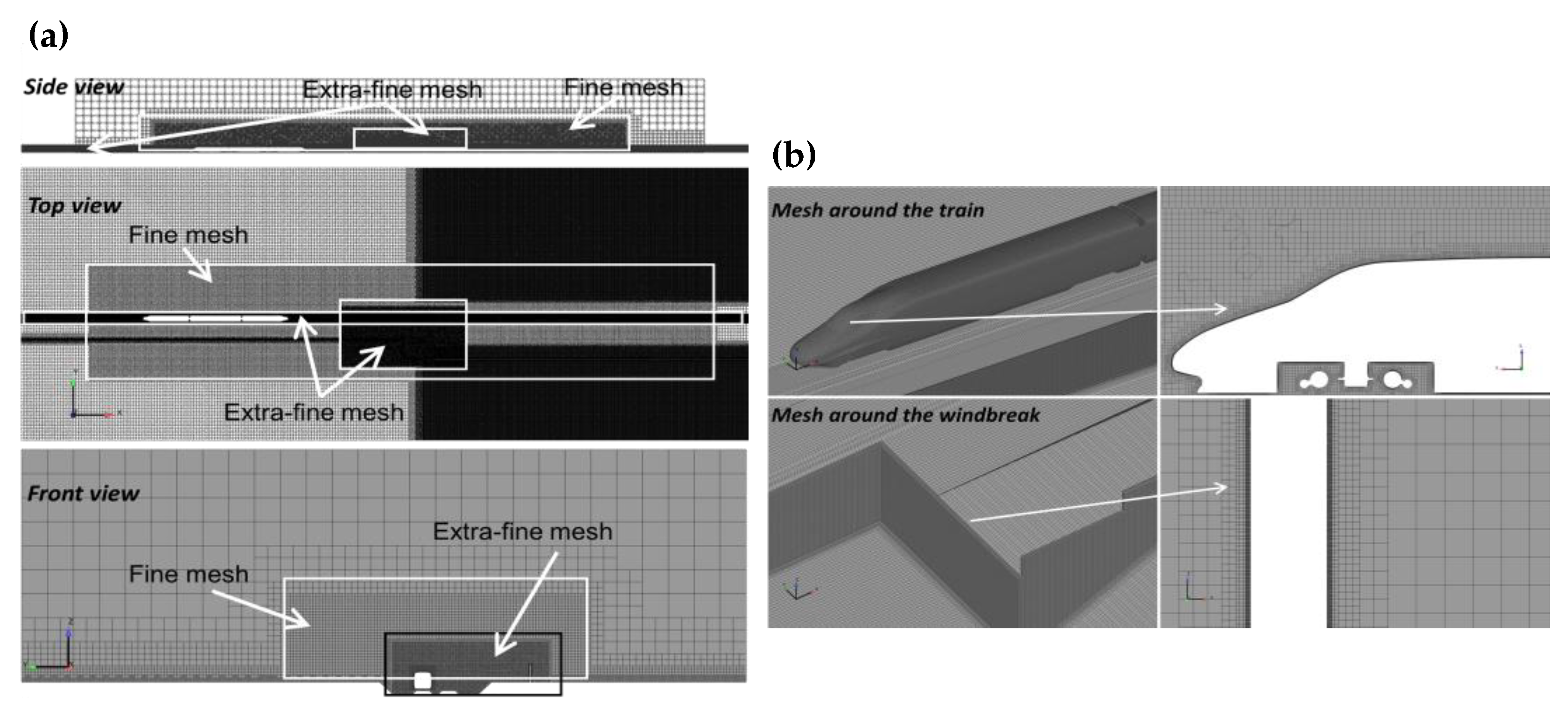
The mesh was an unstructured hexahedral grid generated by OpenFOAM. As shown in Figure 5a, two boxes were used to refine the railway region; a fine mesh was used along the 3/4 length of the railway. The WT region and the sliding mesh domain were set as extra-fine mesh. Figure 5b shows the mesh around the train and windbreak, as well as the corresponding layer meshes. To capture the high gradient velocity change near the wall, ten prism layers were attached to the train surface; the height of the first layer was 0.1 mm, and the average nondimensional wall distance (y+) was approximately 30–40 around the geometry. In Fluent [39], a y+-insensitive wall treatment was embedded into the ω equation to blend the viscous sublayer and the logarithmic layer formulations; therefore, the shear stress in the first cell close to the wall can be determined reliably.
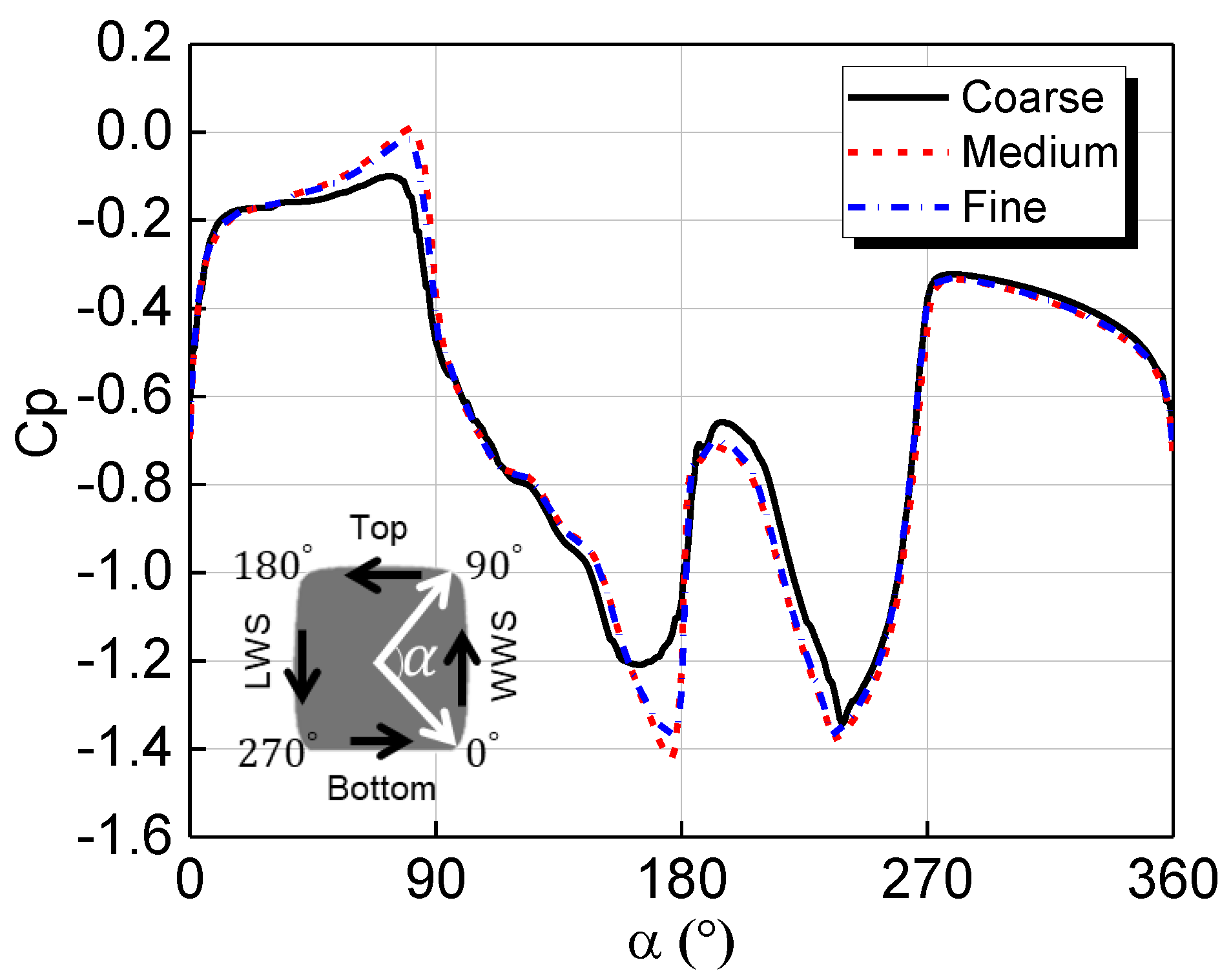
Furthermore, as presented in Table 1, three different mesh resolutions—coarse mesh (22 million), medium mesh (41 million), and fine mesh (64 million)—were considered to avoid the mesh sensitivity. As shown in Figure 6, when the train was stationary in the WT region, the Cp values (defined in Equation (1)) along the middle cross section of the head car were compared for the different mesh resolutions. Due to the poor wind-proofing ability of the WT, the WWS and bottom pressures were greater than those of the LWS and top, respectively, resulting in sudden positive side and lift forces. The three mesh resolutions resulted in a similar phenomenon. However, in both top-corner positions, there was an obvious deviation between the results of coarse mesh and those of medium mesh and fine mesh. Results obtained from the medium and fine meshes were in closer agreement. Therefore, the finer mesh was deemed unnecessary for the simulations, and the medium mesh was used in the present work.

2.4. Data Processing

In this work, non-dimensional coefficients were utilized. As shown in Equation (1), Fy, Fz, and Mx are the side force, lift force, and roll moment, respectively, where ρ is the dry air density under standard atmospheric pressure conditions (101,325 Pa) and the temperatures at 15 °C, which is 1.225 kg/m3, and u is the train speed. A is the reference area, which is 11.22 m2 in the full-scale projected area; and l is the reference length, which is 3 m for the full-scale train. Cp is the pressure coefficient; P is the static pressure on the train surface; and P0 is the reference pressure, which is 0 Pa. In Equation (2), the non-dimensional time t* is used, t is the physical computational time. In Equation (3), U is the non-dimensional velocity obtained from the ratio between the speed of the domain and the crosswind.
CFy = Fy/(0.5 ρu2A); CFz = Fz/(0.5 ρu2A); CMx = Mx/(0.5 ρu2Al); Cp = (P − P0)/(0.5 ρu2)
t* = tu/h
U = Udomain/Ucrosswind

2.5. Results Validation

The time step, grid generation, and mesh independence were selected in Section 2.2 and Section 2.3. The numerical algorithm can be considered to be reliable if results of the numerical simulations were similar to those of wind tunnel tests. Due to the lack of experimental data for comparison with the computational model used in the current work, a previously reported wind tunnel test for a 1:8 scale high-speed train under crosswinds was used for validation [40]. To make the verification more reliable, the same train model and wind tunnel were used in the numerical simulation. The CRH 2 train model was used in this study, so validation was conducted based on the CRH 2 train. Yaw angles from 0° to 19.8° and aerodynamic forces were investigated in an 8 m × 6 m wind tunnel [40]. In the simulation, a resultant wind speed was used to achieve the yaw angle of the test, so the width of the computational domain was wider than that of the experiment, and the length was also longer to allow improved development of the inlet wind. However, the height was identical to that of the wind tunnel test. The numerical method, mesh strategy, and other relative settings were the same as those described above.
Table 2 shows a comparison of aerodynamic forces between the simulation and the test. The maximum deviation between the simulation and the test was less than 5% for the tail car, possibly as a result the complicated flow underneath the tail car. Overall, the comparison results indicate that the relevant numerical settings in the present work are feasible for further CFD analysis. The train’s aerodynamic forces are dominated by the flow structures, indirectly proving that the analysis of average flow structures presented in this paper is acceptable; this indirect approach was also used in previous studies [41].

3. Results, Analysis, and Discussion

3.1. Transient Aerodynamic Forces

Figure 7 shows the aerodynamic forces and moment variations of each car along the WT. The time mark shows the time at which each car passed the WT region. The aerodynamic coefficients exhibited sudden changes in the region of the WT, and the impact of this change was delayed after the WT. In particular, as indicated by the dashed circle in each figure, there was a sudden increase in the values of CFy, CFz, and CMx for each car, although there was a certain distance between this change position and the WT region. The impact of the WT occurred at about t* = 38 for the head car, at about t* = 40 for the middle car, and at about t* = 50 for the tail car. After the impact of WT, the aerodynamic performance recovered to a relatively steady state in the cutting after approximately t* = 85 for the head car, t* = 90 for the middle car, and t* = 100 for the tail car. Therefore, the continuous impact time of the WT was approximately Δt* = 47, Δt* = 50, and Δt* = 50 for the head car, middle car, and tail car, respectively.
The impact times of the WT on each car were similar, but the strongest impact occurred on the right-angle structure of the windbreak, as shown in Figure 7. The aerodynamic forces changed from a minimum to a maximum and then dropped to the minimum value. The transient time (Δt)* of the head car was the shortest, followed by the middle car and the tail car. With respect to the peak-to-peak values of CFy, CFz, and CMx around the right-angle windbreak region, that of the head car was significantly larger than those of the middle car and the tail car. This indicates that the impact of such a WT was more significant for the head car.
Furthermore, as shown in Table 3, in the flat ground and cutting position, the value of CFy for each car was negative, whereas CMx had positive values. This indicates that the backflow was dominant in the flat ground and cutting positions. However, in the WT region, not only was the original steady state broken by the sudden peak value, but the action directions of the aerodynamic loads were opposite to those in the flat ground and cutting positions.

3.2. Transient Flow Structures

3.2.1. Flow Structures on Flat Ground: t* = 47

Before the position of WT at t* = 47 (Figure 8a), the pressure profile on the train body is shown in Figure 8b. As shown in regions A and B, the pressure on the LWS was higher than that on the WWS, especially for the middle car. Thus, the CFy of the middle car had a maximum value of about −0.7 at this time. For the head and tail cars, the CFy values were about −0.4 and −0.2, respectively. Based on the top and bottom pressure distributions, in regions C and D, the pressure at the top was higher than that at the bottom. Thus, the head car’s CFz presented a negative value of about −0.1 at t* = 47. For the middle car in region E, the total pressure difference between the top and bottom was smaller, and the CFz value was close to 0. For the tail car in region F, the pressure of the top position was significantly less than that at the bottom. Consequently, the CFz of the tail car was positive and the largest of the three cars, with a value of approximately 0.4 at this time.
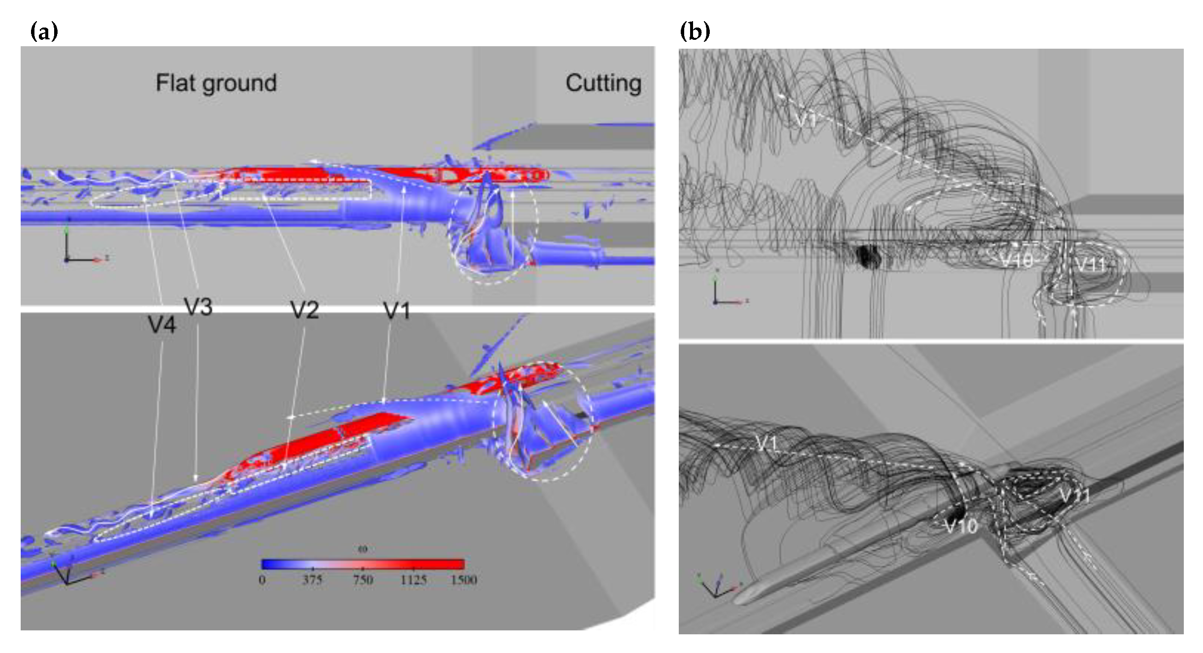
The vortex around the train at t* = 47 is shown in Figure 9. In Figure 9a, the second invariant of the velocity gradient, Q, is used to show the vortices, which are coloured according to the vorticity concentration (ω) [42]. Four vortices are evident around the train, combined with the space streamlines in Figure 9b, the vortex V1 formed due to the space between the WWS of the head car, and the LWS of the windbreak. Vortex V2, which was generated from the lower position of the WWS of the train and V2 in the rear half of the train, was stronger than that in the front half. After the tail car, the V3–V4 generated from the tail car’s nose position and V3 was smoother than V4. After a certain distance, vortices V2, V3, and V4 mixed. A detailed view is shown in Figure 10; strong vortices were induced by the WT, and these vortices increased the side forces on the head and middle cars; however, at this moment, the tail car was influenced by backflows derived from the windbreak walls. Therefore, as shown in Figure 7(a1–a3), at t* = 47, the CFy values of the head and middle cars increased after a step change. Figure 10 shows that the step change for the head car is more sudden, whereas that for the middle car is smoother. In particular, the impact of the vortex induced by the WT on the head car was the strongest and fastest. After the head car, the vortex streamlines impacted the middle car gradually, so the step change of CFy for the middle car was smoother. This phenomenon can be seen clearly in Figure 7.

3.2.2. Flow Structures in the WT Region: t* = 65–48

At t* = 65, when the head car operated in the region of WT, as shown in Figure 11a, there was a region of strong airflow that rushed into the railway in region A and induced an intense positive pressure on the head car’s WWS. The head car’s LWS was surrounded by negative pressures, so the CFy value of the head car (Figure 7(a1)) suddenly became a positive peak value during this time. However, the middle car and tail car were still under the protection effect of the windbreak, so the CFy of the middle car was negative and similar to that at t* = 47, and the CFy of the tail car was also negative and slightly larger than that at t* = 47 due to the impact of extra airflow from the WT region.
The detailed pressure distribution on the train is shown in Figure 11b. Overall, in WWS regions A and B of the head car, the pressure was higher than that in LWS region C. The CFy of the head car was positive. For the middle car (region D) and tail car (region E), it was evident that the LWS pressure was higher than that at the WWS, so their CFy values were still negative. However, because the tail car’s LWS nose part was dominated by strong negative pressures, the CFy of the tail car was less than that of the middle car. The head car’s top pressure became negative and lower than that at the bottom. Thus, the CFz of the head car suddenly became positive in the WT region. In region G of the middle car, the difference between the top and bottom was smaller, and CFz of the middle car was still near zero, similar to that at t* = 47. For the tail car, although the pressure difference for the car body was slight, the pressure on the top of the nose was less than that at the bottom. This resulted in a higher positive CFz value for the tail car, similar to that at t* = 47.
Figure 12a depicts flow structures derived from the train when the head car ran in the WT region At t* = 65. There were new vortices induced by the WT, as indicated by the circle. Furthermore, Figure 12b shows the source of the airflow from the WT. There were mainly two sources. One was from the right-angle region. The direction and magnitude of this part of the airflow changed suddenly near the right-angle structure, and this part of the airflow directly impacted the train, generating vortex V10. The other source is the top position of the slope. The height of the windbreak was insufficient, and this part of airflow rushed into the railway and directly impacted the train, generating vortex V11. Combined with the information presented in Figure 12b, the positions of vortices V10 and V11 corresponded to regions B and A of the head car, respectively. The impact of these two vortices explains why the head car’s CFy showed a sudden peak value in the WT region.
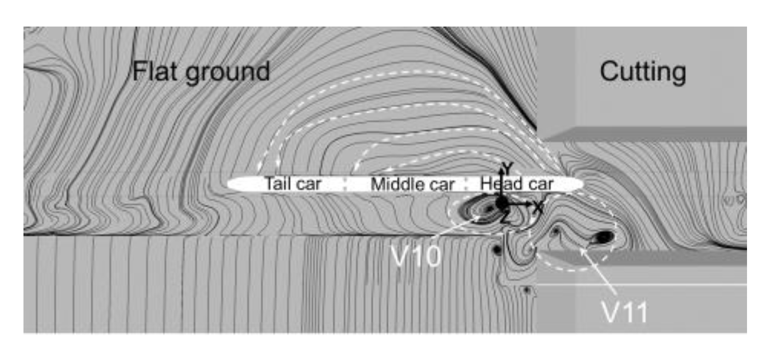
For the detailed flow structures, Figure 13 shows a top view of streamlines around the train and further explains why the head car’s CFy presented a positive change, whereas those of the middle car and the tail car had negative values. Because the entire train was surrounded by a region of backflow from the WT area, the CFy values of the middle car and the tail car were higher than their corresponding values at time t* = 47.
Figure 14 shows the flow field at t* = 75 and t* = 84, respectively, as the train moved through the WT region. At t* = 75, when the middle car was in the WT region, similar to the results at t* = 65, vortices V10 and V11 were generated by the airflow from the right-angle of windbreak (region A) and the top of the slope (B), respectively. In addition, in region C, with the adequate protection of the uniform windbreak and cutting depth, the airflow from region C generated a vortex in the LWS of the train, with no impact on the train. Therefore, the main impact on the train was still in the WT region, and a strong, positive wind speed was evident between vortices V10 and V11. This part of the airflow generated the sudden peak values of CFy for the middle and tail cars. At t* = 84, as the tail car moved away from the right-angle region of the windbreak, the effect of the strong wind speed decreased; then, the train slowly recovered to a steady state. Nevertheless, due to the viscous effect induced by the car body, vortex V11 extended to region D and generated a positive wind speed area on the WWS of the middle car. This resulted in the smallest negative side force for the middle car, as depicted in Figure 7a.

3.2.3. Flow Structures in Cutting Position: t* = 94

The train exited the WT region and ran into the cutting region at t* = 94. Figure 15 shows the pressure distribution around the train. In the cutting position, as shown in Figure 15a, the pressure in region B on the LWS was larger than that in region A of the WWS. Thus, the CFy values of three cars were negative. Furthermore, the pressure was negative in region C in the head car’s WWS and region D in the tail car’s LWS. Therefore, the absolute value of CFy gradually decreased along the train, and a similar pressure distribution phenomenon can be found in Figure 15b. For the pressure distributions at the top and bottom of the train shown in Figure 15b, it is evident that the head car’s pressure difference was smaller. Thus, the CFz was near zero in the cutting position and gradually became positive along the train, especially for the tail car.
Figure 16a displays the flow field around the train in the cutting region at t* = 94. Without the impact of WT, vortex V1 was absent, and only V2–V4 appeared, similar to the flat ground position results. As shown in Figure 16b, vortex V2 generated positive and negative alternating wind speeds in the WWS, and V3–V4 mainly caused a negative wind speed value behind the tail car. In the WT region, a strong vortex and wind speed were generated by the right-angle structure. Figure 17 shows the top view of the flow structure with the train running far from the WT region. Vortices V10 and V11 occurred close to the WT region, similar to when the train operated on flat ground. On the LWS, uniform backflow occurred on the train side. On the WWS, as shown by the dashed, curved arrow, with the effect of vortex V11 and the tail car, a part of airflow moved with the train at the tail of the train, but another portion of the airflow was compressed by the head car and ran opposite to the operation direction of the train. Influenced by these two parts of the airflow, unordered small vortices formed between them.

3.3. Analysis of Vehicle System Dynamic (VSD) Responses

To understand the dynamic characteristics when of train running in the WT region, the dynamic parameters of the train were analysed, as shown in Figure 18. The VSD model of the train used in this paper is the same as that used in our previous work [43]. Other detailed information, including the vehicle system dynamics equation, the definition of dynamic overturning coefficient D (its critical safety value is D < 0.8), the wind load action on the train, etc., can be found in [43]; therefore the detailed VSD model will not be discussed further here.
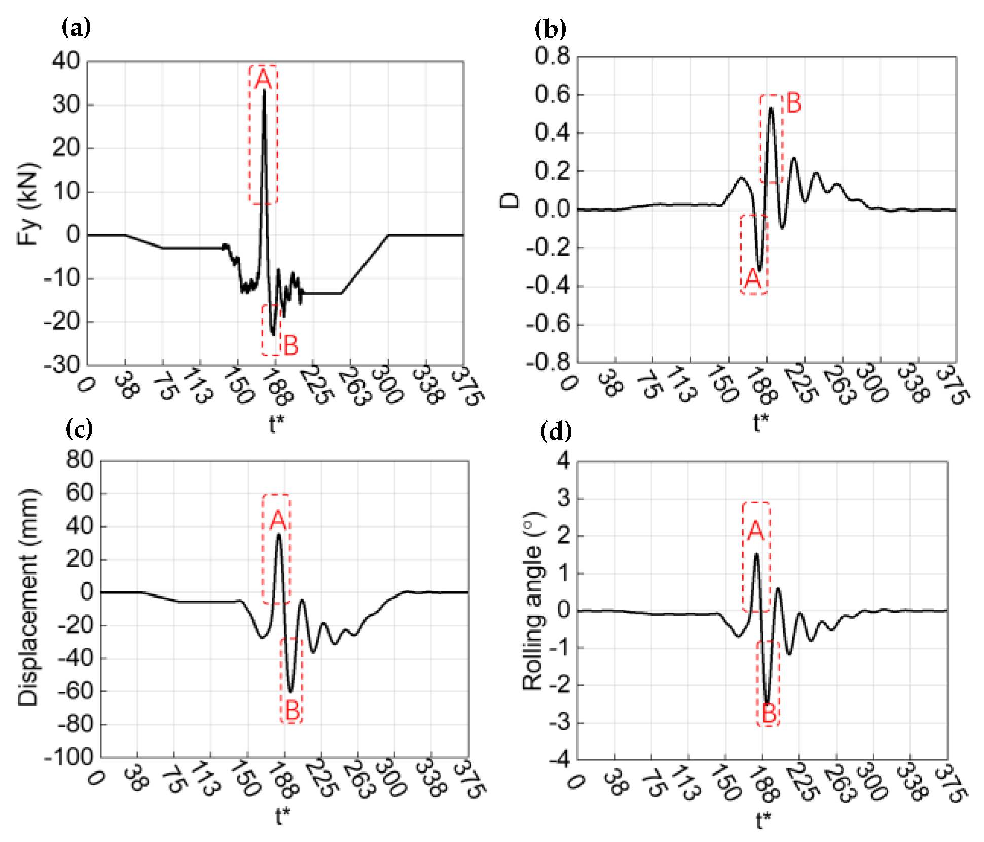
Figure 19a shows the time history of the side force of the head car; extra steady-state values added at the beginning and end position of side force’s time history make the VSD analysis steady, so t* of the horizontal axis in Figure 19 is not consistent with that in Figure 17. Figure 19b–d shows the dynamic overturning coefficient (D), the lateral displacement of the centre of the car body, and the rolling angle. Overall, the peak values of dynamic response in region B and region A were close to each other. Compared with Figure 19a, region A was the position where the positive aerodynamic forces appeared, whereas region B was the location where the aerodynamic forces returned to negative values. This indicates that within a short period, the aerodynamic forces suddenly changed from smaller negative values to larger positive values before finally recovering to the negative values again. In this process, the absolute value of the sudden aerodynamic positive peak was larger than that of the subsequent negative peak value. However, the value of dynamic responses that occurred at the moment the train recovered to the original state is also drastically. Table 4 shows the exact values of the dynamic response parameters. The train always operated safely (D < 0.8), but there was an obvious yawing motion. The absolute value of the maximum (D) was 0.53, the lateral displacement was 60 mm, and the rolling angle was 2.5°.

4. Conclusions and Further Work

Based on three cars and the specific simulated geometric conditions, the impact of windbreak transition (WT) on the train aerodynamic performance and dynamic responses under crosswinds were studied in the current work. The following conclusions were drawn:
  • The impact of the WT was the largest on the head car, and the continuous impact time of the WT was approximately Δt* = 47, Δt* = 50, and Δt* = 50 for the head car, middle car, and tail car, respectively. The sudden wind loads induced by the WT resulted from the position of the right-angle structure and an insufficient height region.
  • The action mechanisms of the WT were the airflow rushed into the railway from the right-angle windbreak region and the slope region, with the airflow directly impacting the train. In particular, two main vortices generated by the WT, V10 and V11, played a key role.
  • The WT region resulted in sudden and continuous dynamic impacts on the train, and the dynamic responses when the train recovered to the original state were also drastically. Under current running conditions, the dynamic overturning coefficients reached to 0.53, the lateral displacement was 60 mm, and the rolling angle was 2.5°.
In the current work, the entire process of aerodynamic and dynamic responses was studied in detail when the train ran through the WT region. Due to the complex terrain along the railway, different structural shapes of WT could be studied in further work. Furthermore, mitigation measures should be investigated to reduce the impact of the WT on the operational safety of trains. In addition, with respect to aerodynamical torques arising on the surface of high-speed trains when they move through the surrounding air medium, including those stemming from both laminar and turbulent regimes under the influence of wind acting on a train in a sideway direction [44,45], investigation of the stability motion of high-speed trains will be conducted in future work. Furthermore, the economic parameters of building structural shapes of WT used in actual engineering should be investigated in future works.

Author Contributions

Z.-W.C.: writing—original draft preparation; E.-Z.R.: data curation and investigation; T.-H.L.: writing—review and editing, supervision, and funding acquisition. Y.-Q.N.: writing—review and editing; X.-S.H.: visualization; Y.-T.X.: validation; W.-H.L.: formal analysis; Z.-J.G.: software and validation; L.Z.: writing—review and editing. All authors have read and agreed to the published version of the manuscript.

Funding

This work was supported by the National Key R&D Program of China (Grant No. 2020YFA0710903), the National Natural Science Foundation of China (Grant No. U1334205), the Open Project of Key Laboratory of Traffic Safety on Track of Ministry of Education, Central South University (Grant No. 502401002), and The Hong Kong Polytechnic University’s Postdoc Matching Fund Scheme (Grant No. 1-W16W).

Institutional Review Board Statement

Not applicable.

Informed Consent Statement

Not applicable.

Data Availability Statement

Not applicable.

Conflicts of Interest

The authors declare that they have no conflict of interest.

References

  1. Chen, Z.; Liu, T.; Jiang, Z.; Guo, Z.; Zhang, J. Comparative analysis of the effect of different nose lengths on train aerodynamic performance under crosswind. J. Fluids Struct. 2018, 78, 69–85. [Google Scholar] [CrossRef]
  2. Hemida, H.; Krajnović, S. LES study of the influence of the nose shape and yaw angles on flow structures around trains. J. Wind Eng. Ind. Aerodyn. 2010, 98, 34–46. [Google Scholar] [CrossRef]
  3. Chen, Z.; Ni, Y.; Wang, Y.; Wang, S.; Liu, T. Mitigating crosswind effect on high-speed trains by active blowing method: A comparative study. Eng. Appl. Comput. Fluid Mech. 2022, 16, 1064–1081. [Google Scholar] [CrossRef]
  4. Dong, X.; Liu, T.; Xia, Y.; Yang, F.; Chen, Z.; Guo, Z. Comparative analysis of the aerodynamic performance of trains and dynamic responses of catenaries for windbreak walls with different heights under crosswind. Proc. Inst. Mech. Eng. Part F J. Rail Rapid Transit 2022, 78, 69–85. [Google Scholar] [CrossRef]
  5. Montenegro, P.; Barbosa, D.; Carvalho, H.; Calçada, R. Dynamic effects on a train-bridge system caused by stochastically generated turbulent wind fields. Eng. Struct. 2020, 211, 110430. [Google Scholar] [CrossRef]
  6. Liu, T.; Wang, L.; Gao, H.; Xia, Y.; Guo, Z.; Li, W.; Liu, H. Research progress on train operation safety in Xinjiang railway under wind environment. Transp. Saf. Environ. 2022, 4, tdac005. [Google Scholar] [CrossRef]
  7. Liu, T.-H.; Wang, L.; Chen, Z.-W.; Gao, H.-R.; Li, W.-H.; Guo, Z.-J.; Xia, Y.-T.; Huo, X.-S.; Wang, Y.-W. Study on the pressure pipe length in train aerodynamic tests and its applications in crosswinds. J. Wind. Eng. Ind. Aerodyn. 2022, 220, 104880. [Google Scholar] [CrossRef]
  8. Gallagher, M.; Morden, J.; Baker, C.; Soper, D.; Quinn, A.; Hemida, H.; Sterling, M. Trains in crosswinds–comparison of full-scale on-train measurements, physical model tests and CFD calculations. J. Wind. Eng. Ind. Aerodyn. 2018, 175, 428–444. [Google Scholar] [CrossRef] [Green Version]
  9. He, X.-h.; Zuo, T.-h.; Zou, Y.-f.; Yan, L.; Tang, L.-b. Experimental study on aerodynamic characteristics of a high-speed train on viaducts in turbulent crosswinds. J. Cent. South Univ. 2020, 27, 2465–2478. [Google Scholar] [CrossRef]
  10. Li, W.; Liu, T.; Martinez-Vazquez, P.; Guo, Z.; Huo, X.; Xia, Y.; Chen, Z. Effects of embankment layouts on train aerodynamics in a wind tunnel configuration. J. Wind. Eng. Ind. Aerodyn. 2022, 220, 104830. [Google Scholar] [CrossRef]
  11. Cheli, F.; Ripamonti, F.; Rocchi, D.; Tomasini, G. Aerodynamic behaviour investigation of the new EMUV250 train to cross wind. J. Wind. Eng. Ind. Aerodyn. 2010, 98, 189–201. [Google Scholar] [CrossRef]
  12. Sicot, C.; Deliancourt, F.; Boree, J.; Aguinaga, S.; Bouchet, J. Representativeness of geometrical details during wind tunnel tests. Application to train aerodynamics in crosswind conditions. J. Wind Eng. Ind. Aerodyn. 2018, 177, 186–196. [Google Scholar] [CrossRef]
  13. Xiang, H.; Li, Y.; Chen, S.; Li, C. A wind tunnel test method on aerodynamic characteristics of moving vehicles under crosswinds. J. Wind Eng. Ind. Aerodyn. 2017, 163, 15–23. [Google Scholar] [CrossRef]
  14. Liu, T.; Chen, Z.; Guo, Z.; Krajnović, S. Reasonable pressure tap layout to measure the aerodynamic forces of a train at different yaw angles. Measurement 2020, 166, 108255. [Google Scholar] [CrossRef]
  15. Dorigatti, F.; Sterling, M.; Baker, C.; Quinn, A. Crosswind effects on the stability of a model passenger train—A comparison of static and moving experiments. J. Wind Eng. Ind. Aerodyn. 2015, 138, 36–51. [Google Scholar] [CrossRef]
  16. Chen, Z.; Ni, Y. Sudden flow induced by mountain ridges beside windbreaks in a railway and its mitigation measures. Transp. Saf. Environ. 2022, 4, tdac004. [Google Scholar] [CrossRef]
  17. Chen, Z.-W.; Liu, T.-H.; Yan, C.-G.; Yu, M.; Guo, Z.-J.; Wang, T.-T. Numerical simulation and comparison of the slipstreams of trains with different nose lengths under crosswind. J. Wind. Eng. Ind. Aerodyn. 2019, 190, 256–272. [Google Scholar] [CrossRef]
  18. Flynn, D.; Hemida, H.; Baker, C. On the effect of crosswinds on the slipstream of a freight train and associated effects. J. Wind Eng. Ind. Aerodyn. 2016, 156, 14–28. [Google Scholar] [CrossRef] [Green Version]
  19. Guo, Z.; Liu, T.; Chen, Z.; Liu, Z.; Monzer, A.; Sheridan, J. Study of the flow around railway embankment of different heights with and without trains. J. Wind. Eng. Ind. Aerodyn. 2020, 202, 104203. [Google Scholar] [CrossRef]
  20. Dong, X.; Liu, T.; Shi, Z.; Xia, Y.; Yang, F.; Chen, Z. Influence of porosity of reformed earth embankment windbreak wall on flow field and displacement of catenary under crosswinds. J. Wind. Eng. Ind. Aerodyn. 2021, 214, 104652. [Google Scholar] [CrossRef]
  21. Zhang, J.; Zhang, M.; Li, Y.; Fang, C. Aerodynamic effects of subgrade-tunnel transition on high-speed railway by wind tunnel tests. Wind. Struct. 2019, 28, 203–213. [Google Scholar] [CrossRef]
  22. Li, Y.; Hu, P.; Cai, C.; Zhang, M.; Qiang, S. Wind tunnel study of a sudden change of train wind loads due to the wind shielding effects of bridge towers and passing trains. J. Eng. Mech. 2013, 139, 1249–1259. [Google Scholar] [CrossRef]
  23. Wu, M.; Li, Y.; Chen, N. The impact of artificial discrete simulation of wind field on vehicle running performance. Wind. Struct. 2015, 20, 169–189. [Google Scholar] [CrossRef]
  24. Lou, P.; Tao, W.; Cai, C.; He, X.; Zou, Y.; Ai, Y. Influence of Wind Barriers with Different Curvatures on Crosswind Aerodynamic Characteristics of a Train-Bridge System. Appl. Sci. 2022, 12, 1747. [Google Scholar] [CrossRef]
  25. Niu, J.; Zhang, Y.; Li, R.; Chen, Z.; Yao, H.; Wang, Y. Aerodynamic simulation of effects of one-and two-side windbreak walls on a moving train running on a double track railway line subjected to strong crosswind. J. Wind. Eng. Ind. Aerodyn. 2022, 221, 104912. [Google Scholar] [CrossRef]
  26. Chen, Z.; Liu, T.; Li, M.; Yu, M.; Lu, Z.; Liu, D. Dynamic response of railway vehicles under unsteady aerodynamic forces caused by local landforms. Wind. Struct. 2019, 29, 149–161. [Google Scholar] [CrossRef]
  27. Huo, X.; Liu, T.; Chen, Z.; Li, W.; Gao, H.; Wang, S. Comparative analysis of the aerodynamic characteristics on double-unit trains formed by different types of high-speed train. J. Wind. Eng. Ind. Aerodyn. 2021, 217, 104757. [Google Scholar] [CrossRef]
  28. Chen, Z.; Liu, T.; Yu, M.; Chen, G.; Chen, M.; Guo, Z. Experimental and numerical research on wind characteristics affected by actual mountain ridges and windbreaks: A case study of the Lanzhou-Xinjiang high-speed railway. Eng. Appl. Comput. Fluid Mech. 2020, 14, 1385–1403. [Google Scholar] [CrossRef]
  29. Niu, J.; Zhou, D.; Liang, X. Numerical investigation of the aerodynamic characteristics of high-speed trains of different lengths under crosswind with or without windbreaks. Eng. Appl. Comput. Fluid Mech. 2018, 12, 195–215. [Google Scholar] [CrossRef]
  30. Sun, Z.; Hashmi, S.A.; Dai, H.; Cheng, X.; Zhang, T.; Chen, Z. Safety comparisons of a high-speed train’s head and tail passing by a windbreak breach. Veh. Syst. Dyn. 2021, 59, 823–840. [Google Scholar] [CrossRef]
  31. Hashmi, S.A.; Hemida, H.; Soper, D. Wind tunnel testing on a train model subjected to crosswinds with different windbreak walls. J. Wind. Eng. Ind. Aerodyn. 2019, 195, 104013. [Google Scholar] [CrossRef]
  32. Chen, Z.; Liu, T.; Zhou, X.; Niu, J. Impact of ambient wind on aerodynamic performance when two trains intersect inside a tunnel. J. Wind. Eng. Ind. Aerodyn. 2017, 169, 139–155. [Google Scholar] [CrossRef]
  33. Mamouri, A.R.; Lakzian, E.; Khoshnevis, A.B. Entropy analysis of pitching airfoil for offshore wind turbines in the dynamic stall condition. Ocean. Eng. 2019, 187, 106229. [Google Scholar] [CrossRef]
  34. Liu, T.; Chen, Z.; Zhou, X.; Zhang, J. A CFD analysis of the aerodynamics of a high-speed train passing through a windbreak transition under crosswind. Eng. Appl. Comput. Fluid Mech. 2018, 12, 137–151. [Google Scholar] [CrossRef] [Green Version]
  35. Deng, E.; Yang, W.; Lei, M.; Zhu, Z.; Zhang, P. Aerodynamic loads and traffic safety of high-speed trains when passing through two windproof facilities under crosswind: A comparative study. Eng. Struct. 2019, 188, 320–339. [Google Scholar] [CrossRef]
  36. Morden, J.A.; Hemida, H.; Baker, C. Comparison of RANS and detached eddy simulation results to wind-tunnel data for the surface pressures upon a class 43 high-speed train. J. Fluids Eng. 2015, 137. [Google Scholar] [CrossRef]
  37. Yao, S.-B.; Sun, Z.-X.; Guo, D.-L.; Chen, D.-W.; Yang, G.-W. Numerical study on wake characteristics of high-speed trains. Acta Mech. Sin. 2013, 29, 811–822. [Google Scholar] [CrossRef] [Green Version]
  38. Menter, F.R. Two-equation eddy-viscosity turbulence models for engineering applications. AIAA J. 1994, 32, 1598–1605. [Google Scholar] [CrossRef] [Green Version]
  39. ANSYS, F. ANSYS Fluent Theory Guide 18.1; ANSYS, Inc.: Canonsburg, PA, USA, 2017; Available online: http://www.ansys.com (accessed on 1 June 2022).
  40. Zhang, L.; Yang, M.-z.; Liang, X.-f. Experimental study on the effect of wind angles on pressure distribution of train streamlined zone and train aerodynamic forces. J. Wind. Eng. Ind. Aerodyn. 2018, 174, 330–343. [Google Scholar] [CrossRef]
  41. Chen, G.; Li, X.-B.; Liu, Z.; Zhou, D.; Wang, Z.; Liang, X.-F.; Krajnovic, S. Dynamic analysis of the effect of nose length on train aerodynamic performance. J. Wind Eng. Ind. Aerodyn. 2019, 184, 198–208. [Google Scholar] [CrossRef]
  42. Wang, J.; Minelli, G.; Dong, T.; Chen, G.; Krajnović, S. The effect of bogie fairings on the slipstream and wake flow of a high-speed train. An IDDES study. J. Wind. Eng. Ind. Aerodyn. 2019, 191, 183–202. [Google Scholar] [CrossRef]
  43. Chen, Z.; Liu, T.; Li, W.; Guo, Z.; Xia, Y. Aerodynamic performance and dynamic behaviors of a train passing through an elongated hillock region beside a windbreak under crosswinds and corresponding flow mitigation measures. J. Wind Eng. Ind. Aerodyn. 2021, 208, 104434. [Google Scholar] [CrossRef]
  44. Ershkov, S.V. Non-stationary Riccati-type flows for incompressible 3D Navier–Stokes equations. Comput. Math. Appl. 2016, 71, 1392–1404. [Google Scholar] [CrossRef]
  45. Miloh, T.; Landweber, L. Generalization of the Kelvin–Kirchhoff equations for the motion of a body through a fluid. Phys. Fluids 1981, 24, 6–9. [Google Scholar] [CrossRef]
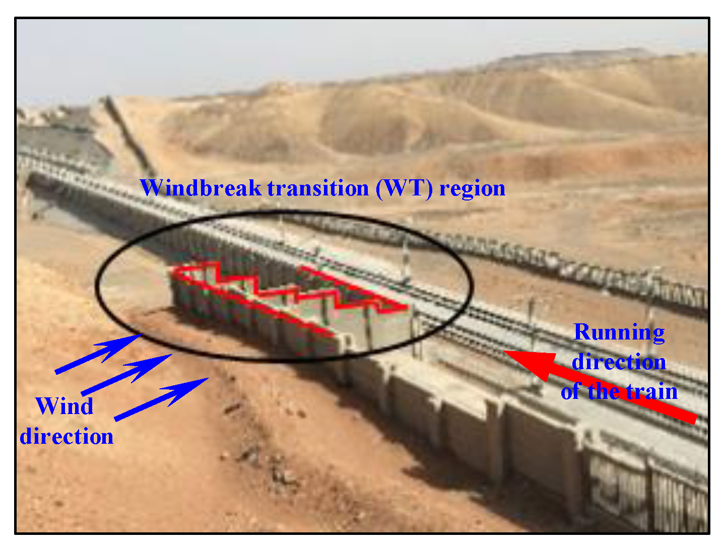
Figure 1. WT region on an actual high-speed railway.
Applsci 12 07217 g001
Figure 2. WT region in the study simulation.
Applsci 12 07217 g002
Figure 3. High-speed train model.
Applsci 12 07217 g003
Figure 4. Computational domain and boundary conditions.
Applsci 12 07217 g004
Figure 5. Computational mesh: (a) different views and (b) the mesh around the model and the surface layer mesh.
Applsci 12 07217 g005
Figure 6. Comparison of different mesh resolutions.
Applsci 12 07217 g006
Figure 7. Aerodynamic forces and moment variation along the WT: (a1a3) CFy of head car, middle car and tail car, respectively, (b1b3) CFz of head car, middle car and tail car, respectively, and (c1c3) CMx of head car, middle car and tail car, respectively.
Applsci 12 07217 g007
Figure 8. Pressure distribution on the train surface at t* = 47: (a) train position and (b) pressure distribution.
Applsci 12 07217 g008
Figure 9. Flow structures around the train at t* = 47: (a) vortex distribution (Q = 5000) and (b) space streamlines.
Applsci 12 07217 g009
Figure 10. Top view of streamlines at a height 0.5 h.
Applsci 12 07217 g010
Figure 11. (a) The distribution of the wind speed coefficient (U) at a height of 0.5 h and (b) pressure distribution on the train surface.
Applsci 12 07217 g011
Figure 12. Flow structures around the train at t* = 65: (a) vortex distribution (Q = 5000) and (b) space streamlines.
Applsci 12 07217 g012
Figure 13. Top view of the streamlines at a height of 0.5 h.
Applsci 12 07217 g013
Figure 14. Flow structures and speed contours around the train at different times: (a) t* = 75 and (b) t* = 84.
Applsci 12 07217 g014
Figure 15. Pressure distribution at t* = 94: (a) top view at a height of 0.5 h and (b) train surface.
Applsci 12 07217 g015
Figure 16. Flow field distribution at t* = 94: (a) vortex around the train (Q = 5000) and (b) velocity distribution at a height of 0.5 h.
Applsci 12 07217 g016
Figure 17. Top view of streamlines at a height of 0.5 h.
Applsci 12 07217 g017
Figure 18. Vehicle dynamic model: (a) bogie model and (b) entire train model.
Applsci 12 07217 g018
Figure 19. Dynamic response time history: (a) side force (Fy), (b) overturning coefficient (D), (c) lateral displacement, and (d) the rolling angle of the car body centre.
Applsci 12 07217 g019
Table 1. Details of the different grid resolutions.
ItemCoarseMediumFine
Number of volume meshes/million224164
Size of the smallest mesh on train surface/mm3.11–1.60.96
Number of prism layers101010
First boundary layer/mm0.310.1–0.160.096
Table 2. Comparison of the side and lift force coefficients between the wind tunnel tests and simulations under a crosswind at a yaw angle of 19.8°.
CFyCFz
Head CarMiddle CarTail CarHead CarMiddle CarTail Car
Test1.9320.9420.3021.9991.4641.198
Numerical2.0100.9570.3122.0121.4801.253
Error4.04%1.59%3.31%0.65%1.09%4.59%
Table 3. Aerodynamic coefficient in different positions along the WT.
Flat GroundTransition Region:
Maximum Sudden
Peak Value
Cutting
Head CarMiddle CarTail CarHead CarMiddle CarTail CarHead CarMiddle CarTail Car
CFy−0.20−0.50−0.101.000.300.48−0.40−0.220.00
CFz−0.14−0.020.380.210.360.400.020.100.20
CMx0.030.280.10−0.56−0.20−0.280.180.100.00
Table 4. Value of the maximum dynamic responses.
DLateral Displacement (mm)Rolling Angle (°)
Maximum positive value0.53351.55
Maximum negative value−0.32−60−2.5
Peak-to-peak value0.85954.05
Publisher’s Note: MDPI stays neutral with regard to jurisdictional claims in published maps and institutional affiliations.