Abstract
Given the problems of low accuracy and complex process steps currently faced by the field of fault diagnosis, a fault diagnosis method based on multi-sensor data weighted fusion (MSDWF) combined with depth-wise separable convolutions (DWSC) is proposed. The method takes into account the temporal and spatial information contained in multi-sensor data and can realize end-to-end bearing fault diagnosis. MSDWF is committed to comprehensively characterizing the state information of bearings, and the weighted operation of the multi-sensor data is to establish the interactive information to tap into the inline relationship in the data; DWSC equipped with residual connection is used to realize the decoupling of the channel and spatial correlation of the data. In order to verify the proposed method, the data obtained by a different number of sensors with weighted and unweighted states are used as the input of DWSC, respectively, for comparison, and finally, the effectiveness of MSDWF is verified. Through the comparison between different fault diagnosis methods, the method based on MSDWF and DWSC shows better stability and higher accuracy. Finally, when facing different experimental datasets, the method has similar performance, which shows the stability of the method on different datasets.
1. Introduction
With the improvement of the degree of mechanization, mechanical equipment failure has become a problem that cannot be ignored and will bring significant safety accidents and economic losses. A large proportion of all mechanical equipment failures are caused by bearing failures [1]. In industry, bearings, as one of the essential parts of machines, are often used in a variety of mechanical equipment. They are often faced with complex working conditions, which results in various types of bearing failures. To avoid mechanical equipment damage caused by bearing faults, more and more scholars pay attention to bearing fault diagnosis [2,3,4].
For many years, many effective methods have been put forward in the research of fault diagnosis [5,6,7]. Poongodi et al. [8] collected the sound signals of gears under different loads and speeds and extracted kurtosis, root means square (RMS), standard deviation (SD), and other distinctive features of the signals from the different signal domains to identify the faulty of the gear. Wang et al. [9] proposed to obtain prominent features to construct the initial feature set, then t-distributed Stochastic Neighbor Embedding (t-SNE) and other methods were applied to reduce the correlation of the initial features and characterize the local information of the dataset, and finally input the obtained low-dimensional sensitive feature subset into the k-nearest neighbor classifier (KNNC) for fault classification. Obviously, the methods mentioned above have cumbersome steps of feature extraction, which greatly lower the efficiency of fault diagnosis and cannot be widely applied and keep up with the fast technological development.
With the vigorous development of computer techniques, deep learning (DL) rises in response to the proper time and conditions, and so fault diagnosis combined with DL has become popular [10,11,12]. Zhao et al. [13] proposed to combine convolutional neural networks (CNN) with batch normalization (BN) and the exponential moving average technology to solve the problems of complex working conditions and imbalanced datasets. The method has good accuracy and robustness. Zhao et al. [14] proposed to embed soft thresholding into the structures as nonlinear transformation layers to remove noise effects and integrate specific neural networks (NN) to adaptively adjust the threshold, which effectively improved the ability of feature learning to previous DL methods and obtain high accuracy for fault recognition of vibration signals in high noise environments. Liang et al. [15] integrated dilated convolution network with a residual connection to process time domain vibration signals. The above methods combined with DL promote efficiency and decrease the complicated procedures of fault diagnosis. However, it only utilizes the signal of a single state or a single sensor for fault diagnosis, which makes it difficult to fully express the rich features contained in the raw signal.
In some studies, scholars have proposed methods combining the data fusion method and DL for fault recognition [16,17,18]. Mao et al. [19] propose to combine the signal information from three domains into the matrix with three rows and input the matrix to a pre-trained VGG-16 model, which can distinguish the different bearing defects precisely and achieve the online monitoring of early bearing failure effectively. Li et al. [20] proposed to extract permutation entropy (PE) from multi-sensor data and input multiscale permutation entropy (MPE) into multi-channel CNN (MCCNN). Jing et al. [21] proposed an adaptive data fusion method based on multi-sensor data and different fusion levels. Min et al. [22] proposed to input the data obtained from multiple sensors into CNN to accomplish the end-to-end fault diagnosis.
The above research on multi-sensor and multi-state data fusion has achieved many successes and raised the fault diagnosis accuracy to some extent. However, there are the following problems: (1) It is not considered that the interference information produced by the strong noise and variable working conditions will distort the signal, and the weak features will be drowned. (2) MCCNN utilized to process multi-sensor or multi-state data does not achieve complete decoupling of the channel and spatial correlation [23]. Based on the above reasons, the paper proposes the method of bearing fault diagnosis based on DWSC and MSDWF. The general idea of the method is as follows: the time series data obtained by different sensors are weighted by the self-attention method (SAM). The similarity matrix of time series data is extracted from the data themselves by SAM to achieve the weighting of the original data, which strengthens the weak features in the signal and weakens the influence of the interference information caused by the strong noise and variable working conditions. DWSC equipped with residual connection is to perform depth-wise convolutions (DWC) and point-wise convolutions (PWC) on the weighted multi-sensor data. Among them, the DWC uses a convolution kernel to process the data of one sensor to realize the decoupling of channel correlation, and then PWC is used to process all data. Through the affine transformation of the features, PWC not only decreases the number of parameters involved in the whole operation but also realizes the decoupling of spatial correlation. In MCCNN, one convolution kernel is used to process data of multiple channels, so only incomplete decoupling of the channel and spatial correlation can be achieved, which is the most significant difference between them. The method based on MSDWF and SAM obtains the utmost out of the spatial and temporal information in multi-sensor data and can realize end-to-end fault diagnosis effectively and efficiently.
2. Basic Method
2.1. SAM
SAM is the unique attention mechanism (AM) that is the theory in natural language processing (NLP). AM is to imitate the way humans think when they observe things [24]. That is, when people observe things, to fully use computing resources, they will automatically ignore unimportant information and focus more on information that is more important to the target. Its essence is a method of data weighting. By increasing the weighting of important information and reducing the weighting of interference information, limited computing resources can be reasonably utilized to process the information efficiently. The mathematical expression for the method is as follows:
where represents Query, that is, the information of the entire text, represents Key, that is, the prompt information of the text, represents Value, that is, the content obtained according to the prompt information, and represents the length of the text information, which is a scaling factor used to normalize data.
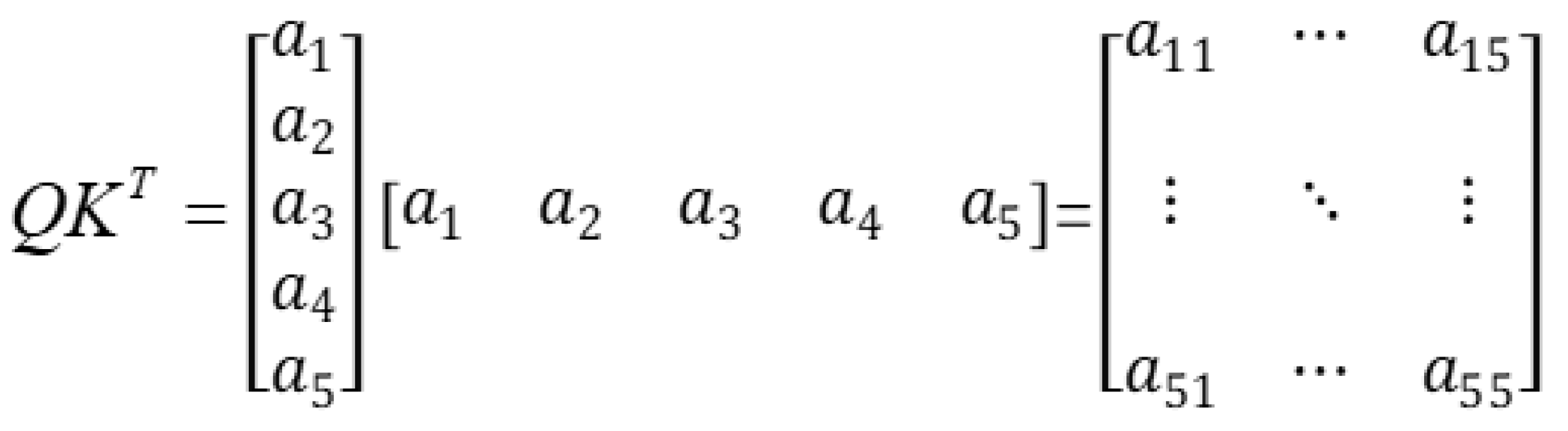
SAM is unique AM that calculates the similarity between data located at different positions in the vector to obtain the intrinsic relationship between these data. In the SAM, the value of Q is equal to K and V. The original input vector is used to obtain the inline relationship between its data. In SAM, QKT represents that the original input vector is multiplied by its transposed vector to obtain a similarity matrix. In the matrix, each row represents the similarity between data at different positions in the vector, as shown in Figure 1.

Figure 1.
Similarity matrix in self-attention mechanism.
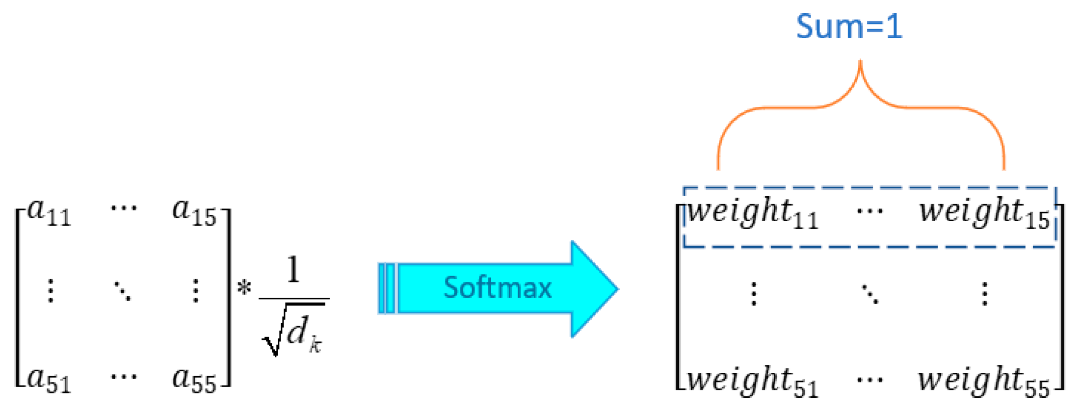
The matrix is scaled by the scaling factor and normalized by Softmax to make the sum of data in each row of the matrix one. The resulting matrix is the weighting matrix, as shown in Figure 2.
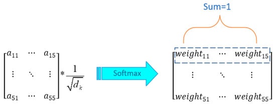
Figure 2.
Weighting matrix in self-attention mechanism.
In the end, the weighting matrix is multiplied by the original input vector to obtain the final weighted vector.
2.2. Depth-Wise Separable Convolutions
DWSC is an improved convolution model for MCCNN. It consists of DWC and PWC, by which the channel and spatial correlation are completely decoupled, and better diagnosis results are achieved [25].
In DWSC, DWC is to convolve each sensor data independently. That is, a convolution kernel calculates only the data of one channel, thereby realizing the mapping of cross-channel correlation and decoupling the channel correlation. Therefore, the number of input and output channels is equal, and then the data are processed by PWC for the next operation. The size of the convolution kernel in DWC is generally 3 × 3.
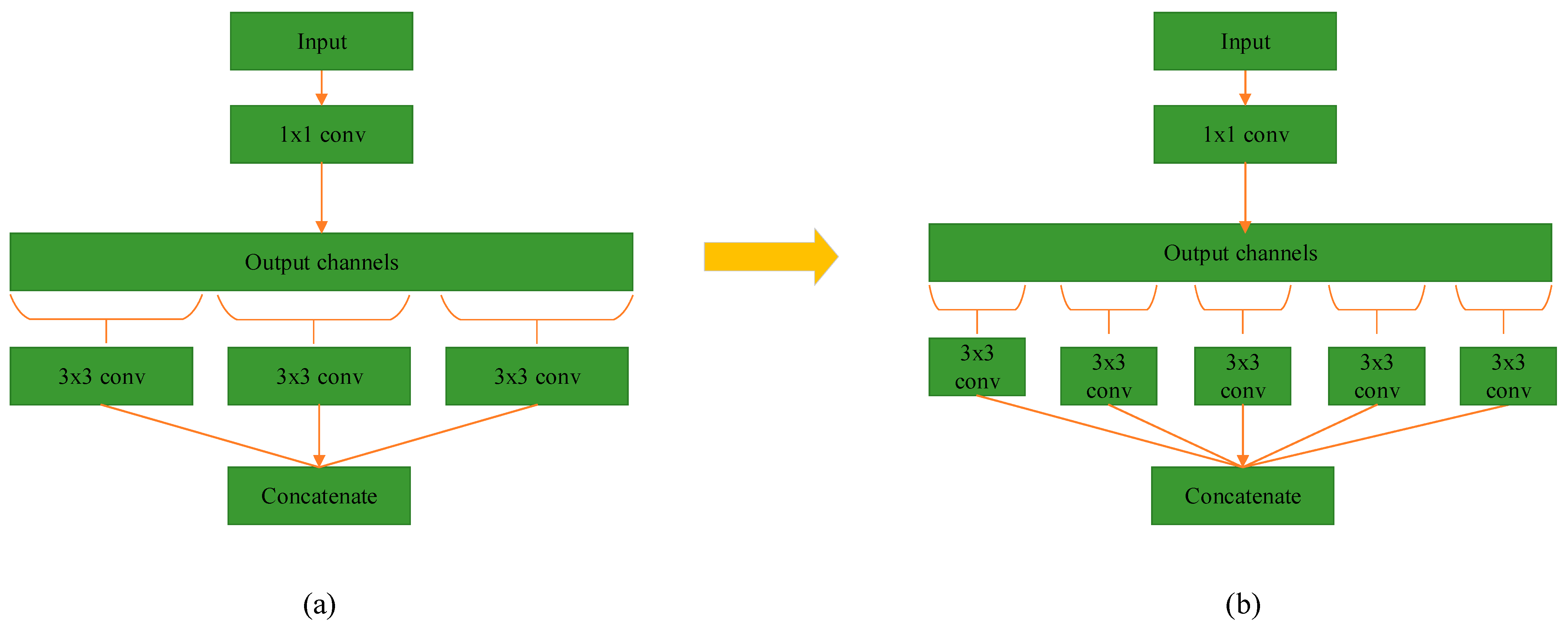
PWC is processed by the 1 × 1 convolution kernel on all channels simultaneously, which realizes the mapping and decoupling of spatial correlation and can also reduce the number of parameters involved in the whole operation. DWSC achieves complete decoupling of cross-channel and spatial correlations through DWC and PWC. In MCCNN, a convolution kernel usually processes data of multiple channels, which decouples cross-channel and spatial correlation to a certain extent but does not achieve complete decoupling, which is the most significant difference between the two methods. The specific comparison between the two methods is shown in Figure 3.
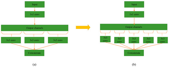
Figure 3.
(a) Multi−channel convolution, (b) depth−wise separable convolutions.
It should be noted that the sequence of 1 × 1 convolution and 3 × 3 does not affect the performance of DWSC. The paper uses the operation sequence of the first DWC.
3. Proposed Method Based on MSDWF and DWSC
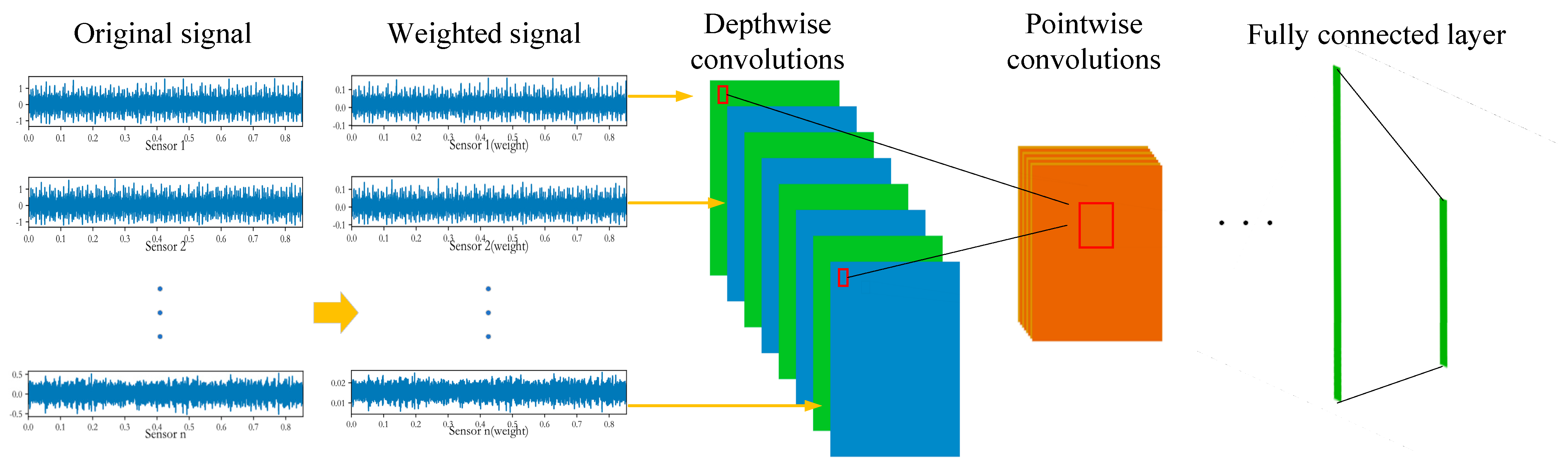
The proposed basic structure based on MSDWF and DWSC is shown in Figure 4. Its structure consists of SAM, DWSC equipped with a residual connection, convolutions, BN, pooling, and Sigmoid, and a fully connected layer (FCL). The bearing vibration signal is a time series vector, and its internal data have an extremely high correlation. For the multi−sensor vibration signals obtained by different sensors, SAM is first used to find out the associated information between the internal data of the vibration signal and strengthen the interaction information between the data to obtain the signal sequence with more obvious characteristics. Then, the weighted data of each sensor are convoluted by DWC respectively to fully extract the unique features and realize the decoupling of the channel correlation of the multi−sensor data. Then the output results are processed by PWC to obtain the spatial features hidden in the multi−sensor data and to completely decouple the spatial correlation. The detailed fault diagnosis structure based on MSDWF and DWSC can be seen as follows:
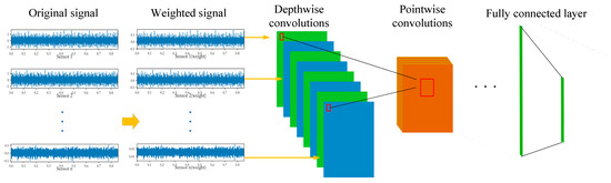
Figure 4.
The architecture of proposed method.
Step 1: Sensors are arranged at different positions of mechanical equipment to obtain vibration signal information at different spatial positions. When the number of sensors arranged is , the obtained vibration data can be indicated as , where represents the data obtained by the th sensor.
Step 2: The data obtained by each sensor are input into SAM for weighting, in which a group of sensor data as a vector sequence is weighted, and the weighted data can be expressed as , where represents the weighted data of the th sensor.
Step 3: The weighted data are divided into two sets for training and test, and then the training data are input into DWSC to realize the decoupling of channel correlation and spatial correlation. After that, the rich features extracted by DWSC are subject to a series of operations such as convolution, BN, pooling, and Sigmoid to characterize the advanced features further. Then, FCL is used to process the obtained advanced features for classification.
Step 4: The test data are input into the trained model for testing and to obtain the test results and analyze the results.
Step 5: The different comparative experiments were carried out to verify the advantage and performance of the method proposed in the paper, and the contrast results were analyzed.
4. Experiment Validation
In order to thoroughly verify the performance of the model proposed, two types of bearing datasets were used for verification. The first type of dataset is the vibration signal of the rolling bearing from Case Western Reserve University (CWRU). The second type is the accelerated life experimental data of the rolling bearing from the rotor bearing laboratory of Xi’an Jiaotong University (XJTU). The two experiments were conducted to compare the differences in fault diagnosis results between the different number of sensors, weighted and unweighted data, and other fault diagnosis methods.
4.1. Case 1: Bearing Fault Diagnosis Based on CWRU Bearing Datasets
4.1.1. Experiment Setup and Data Description
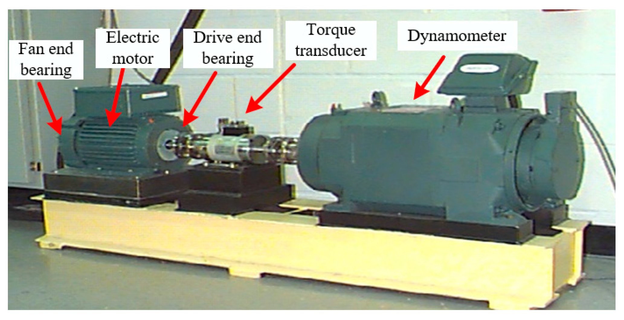
The experimental equipment of CWRU is shown in Figure 5. It consists of a power meter, a torque sensor, an acceleration sensor, and a 2-horsepower motor. In the experiment, three sets of sensor data were obtained by placing the sensors at the motor supporting base and at the twelve o’clock direction of both the fan end (FE) and drive end (DE) of the motor housing. By electro discharge machining, 7, 14, and 21 mils diameter faults were introduced to SKF bearings. The faults were located in three, six, and twelve o’clock directions of the inner race, ball, and outer ring, respectively. The sampling frequency is 12 K and 48 K.

Figure 5.
The experimental platform of CWRU.
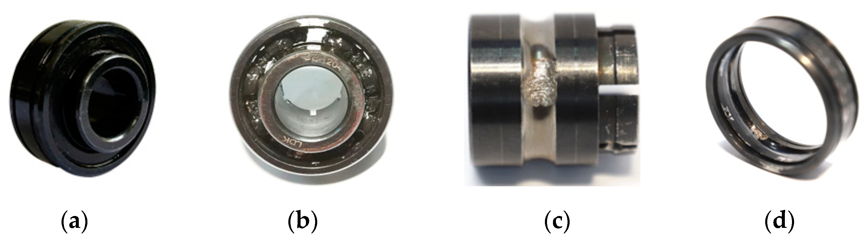
The data used in the experiment are one of DE with the sampling frequency of 12 K. The ball pass frequency on the outer race (BPFO) of the experimental bearing is 104.56 Hz, ball pass frequency on the inner race (BPFI) is 157.94 Hz, and ball spin frequency (BSF) is 137.48 Hz. The selected fault types are inner race, ball, and outer race faults in the six o ‘clock direction. The selected fault diameter is 7 and 14 mils diameter faults, and the motor load is 0 and 1 horsepower (HP). There are nine different failure types in the experiment. Each type of bearing failure can be seen in Figure 6. A total of 2700 samples were selected from three sets of sensor data with 1024 data as one sample, and the number of samples in each set of sensor data is 900. In order to verify the proposed method, three samples were selected from three sets of sensor data, respectively, and the three selected samples were merged into a matrix with three rows and 1024 columns. That is, the number of the new sample is 900, of which 80% were used for training and 20% for tests. A detailed and specific description of the data used in the experiment of CWRU is listed in Table 1.

Figure 6.
Bearing fault. (a) normal, (b) cage fracture, (c) inner race wear, (d) outer race wear.

Table 1.
Experimental datasets of CWRU.
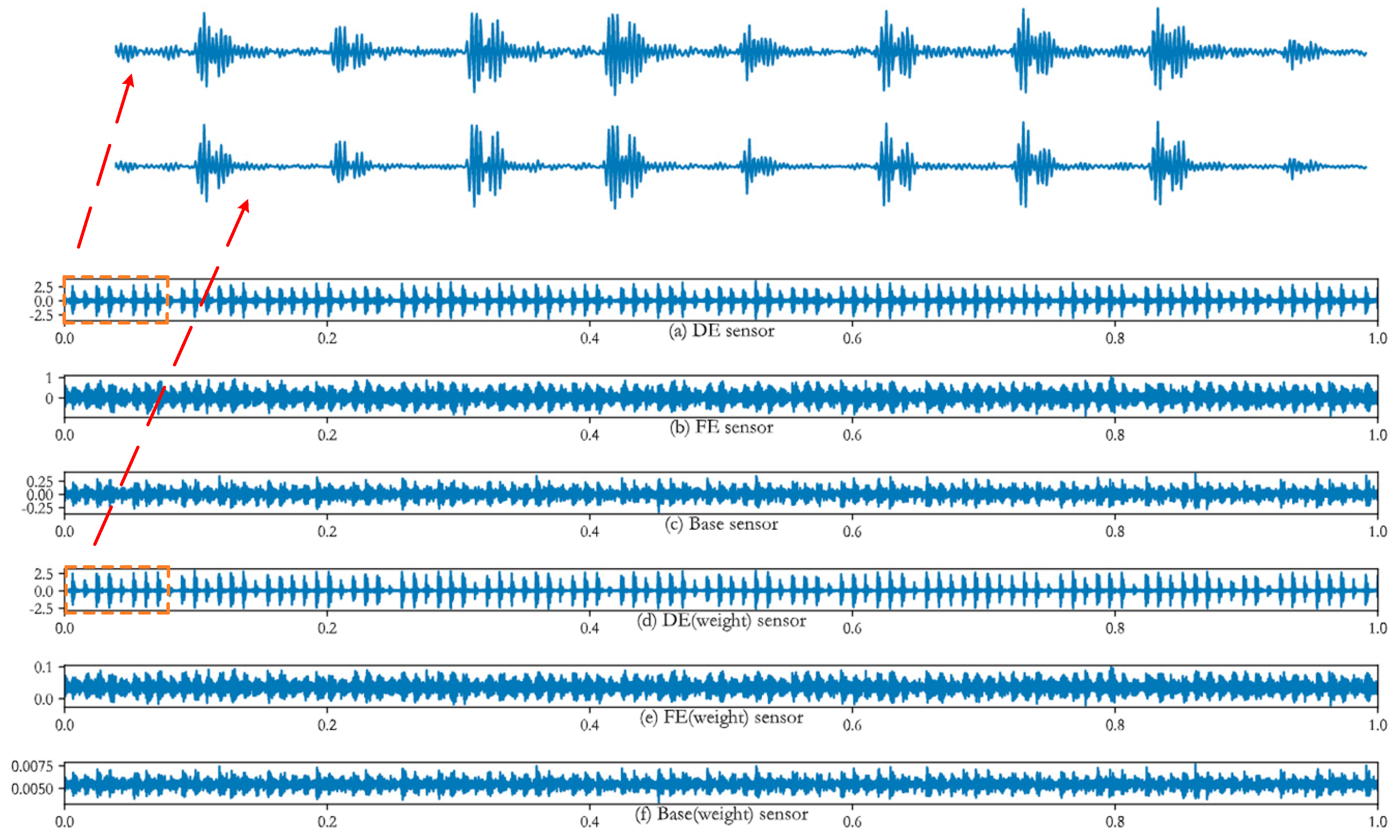
For the original multi-sensor data, the SAM is used to weight them first to obtain the time series data with more obvious features, which is to facilitate the subsequent convolution operation to extract more typical and representative features. As shown in Figure 7, the outer race fault data with no motor load and the fault diameter of 7 mils are selected to compare the time domain graphs of the unweighted and weighted. By comparing the time domain graphs composed of the first 1024 points of the data in Figure 7a,d, it can be observed that by weighting, the waveforms of the data with high similarity in the signal become more unified, the characteristics of the signal become more obvious, and the overall waveform of the signal becomes more regular and symmetrical.
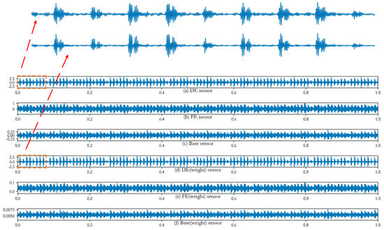
Figure 7.
Time domain graph of outer race fault. (a−c) are the unweighted data obtained by the sensors located at DE, FE, and base, respectively, (d−f) are the corresponding weighted data.
4.1.2. Model Parameters and Results Analysis
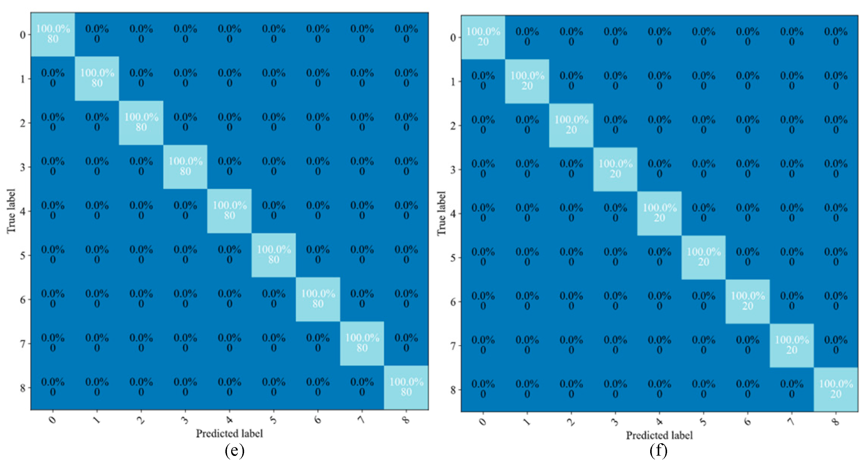
The data weighted by the SAM are input into DWSC for DWC and PWC, as well as the subsequent convolution, BN and pooling, Sigmoid, and classification. The model parameters are given in Table 2. The results of training and testing of the proposed model on CWRU datasets are shown in Figure 8. Figure 8a,b show changes in the accuracy and loss of training and testing datasets with epoch, respectively. As can be seen in Figure 8, when the epoch is about 15 times, the model basically reaches convergence, and the change of accuracy and loss tends to be basically stable. The highest fault diagnosis accuracy rate is 100%. Figure 8c,d are the visualization results by t-SNE, Figure 8c is the visualization graph of the training result, and Figure 8d is the visualization graph of the test result. It can be seen that diverse fault types are almost perfectly separated in Figure 8c,d. Figure 8e,f are the confusion matrix of the training and test results. It can be observed that for the nine fault types, the proposed model can identify and classify them perfectly, and the recognition accuracy of each type of fault is 100%.
Table 2.
Structure and parameters of DWSC and other layers.
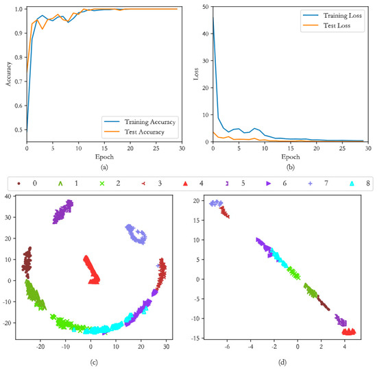
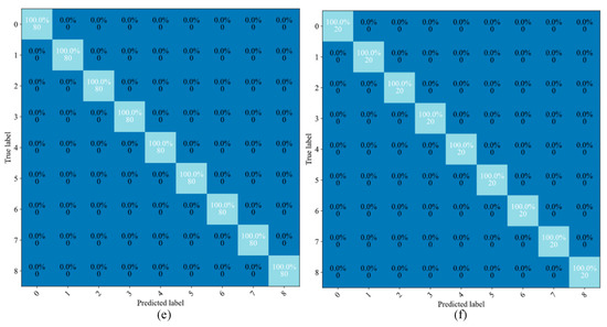
Figure 8.
Training and test results. (a,b) are the changes of the accuracy and loss of the training and testing datasets with epoch, (c,d) are the visualization results of the training and testing results by t-SNE, (e,f) are the confusion matrix of the training and test results.
4.1.3. Comparison between Different Number of Sensors
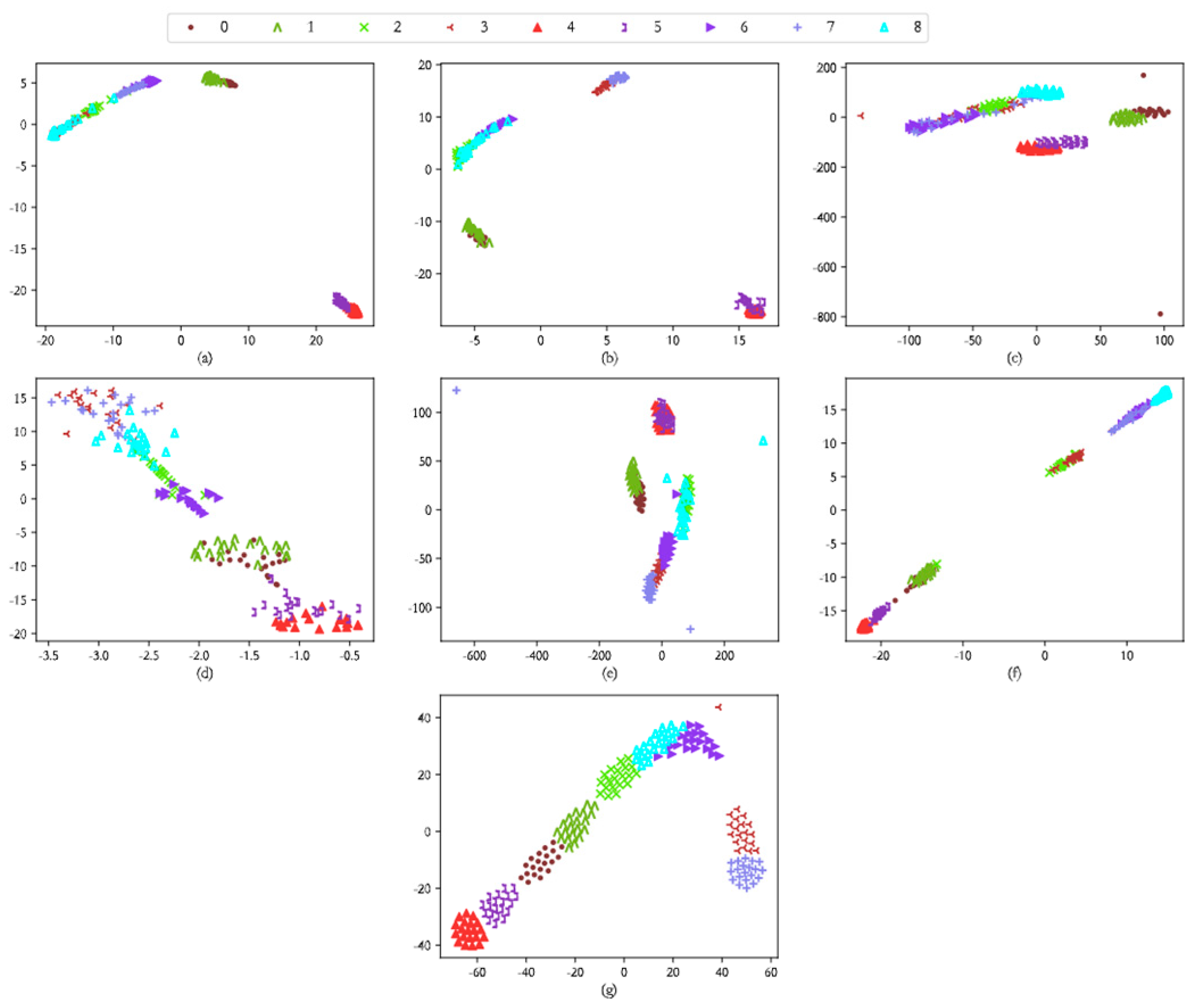
To further test the performance of MSDWF, the signals obtained by different numbers of sensors were input into DWSC to compare the fault diagnosis accuracy. Each sensor data have two states: weighted and unweighted. That is, a total of seven different curves are shown in Figure 9. It can clearly be seen that the weighted single sensor data have higher accuracy and faster convergence rate than the unweighted data and the weighted data fusion of all sensors has the highest accuracy, fastest convergence rate, and best stability, which indicates the superior performance and advantages of the method. In addition, the t-SNE visualization results of different kinds of input data are shown in Figure 10. Figure 10a–c are the visualization results of the weighted data of the base sensor, FE sensor, and DE sensor, respectively, which show a high degree of separation for each fault type, but a small part of the different fault types is still mixed; Figure 10d–f are the visualization results of the unweighted data, and it can be observed that the most of all the fault types are mixed. Compared with the weighted data, there is no good recognition between various types of faults of unweighted data; Figure 10g is the t-SNE visualization result of the weighted data of all sensors, and there is the highest degree of separation for each type of bearing fault.
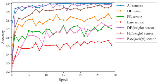
Figure 9.
Comparison of recognition accuracy between the different types input.
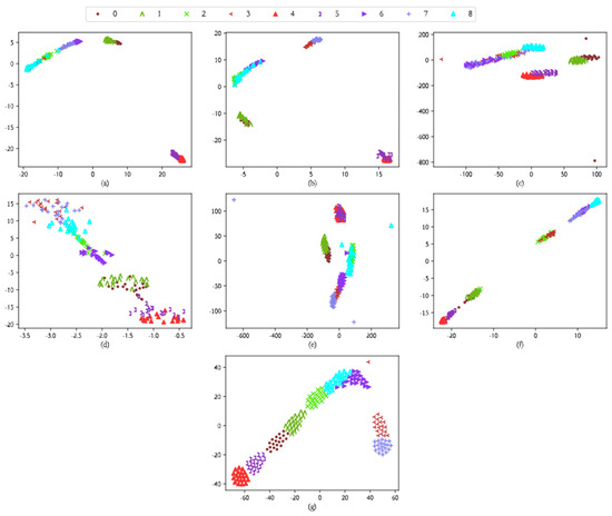
Figure 10.
Visualization result of t-SNE dimensionality reduction. (a–c) are the t-SNE visualization results of the weighted data of the base sensor, FE sensor and DE sensor respectively, (d–f) are the t-SNE visualization results of the unweighted data, (g) is the t-SNE visualization result of the weighted data of all sensors.
4.1.4. Comparison between Different Methods
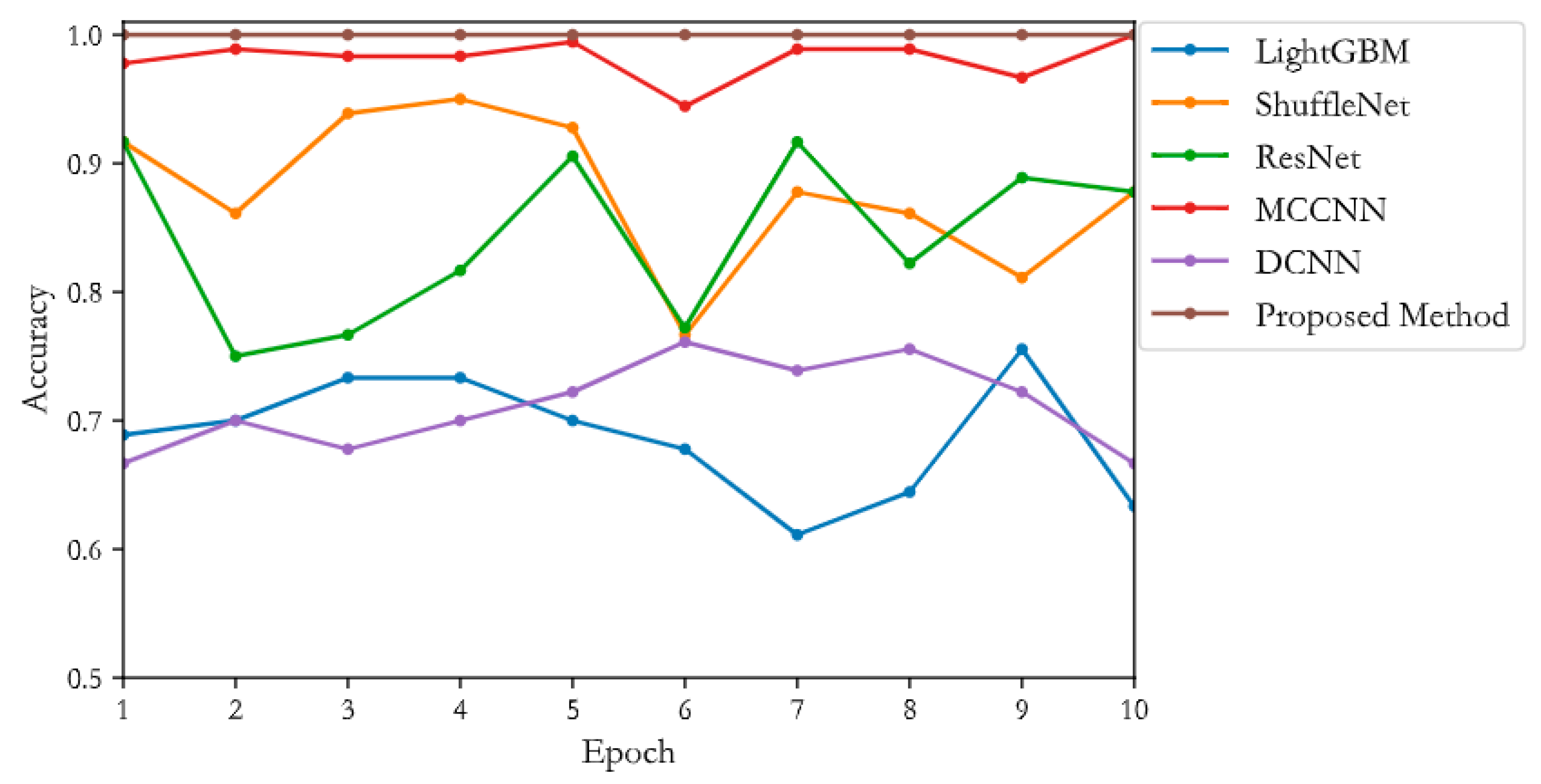
To test the differences between DWSC and other methods, such as Resnet, DCNN, ShuffleNet, MCCNN, and boosting type of integrated algorithm Light Gradient Bosting Machine (LightGBM) that has eminent performance in the field of machine learning, a total of ten comparative experiments were conducted, and the comparative results of accuracy are shown in Figure 11. The average value and SD of fault classification accuracy of each method in ten experiments are listed in Table 3. The average accuracy of DWSC is 100%, followed by MCCNN, with an average accuracy of 98.17% and SD of 0.015. ShuffleNet and ResNet have similar accuracy, 87.89% and 84.33%, with SD of 0.055 and 0.062, respectively. DCNN and LightGBM have the lowest accuracy, 71.11% and 68.78%, with SD of 0.033 and 0.046, respectively.
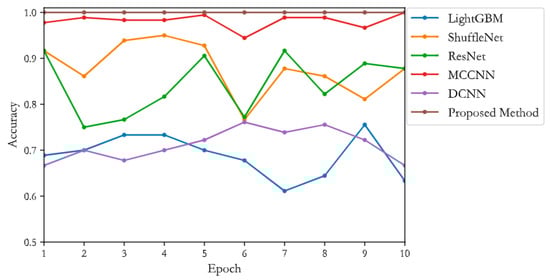
Figure 11.
Comparisons between the different fault diagnosis methods.
Table 3.
Average accuracy and SD of the different methods.
4.2. Case 2: Bearing Fault Diagnosis Based on XJTU Bearing Datasets
4.2.1. Experiment Setup and Data Description
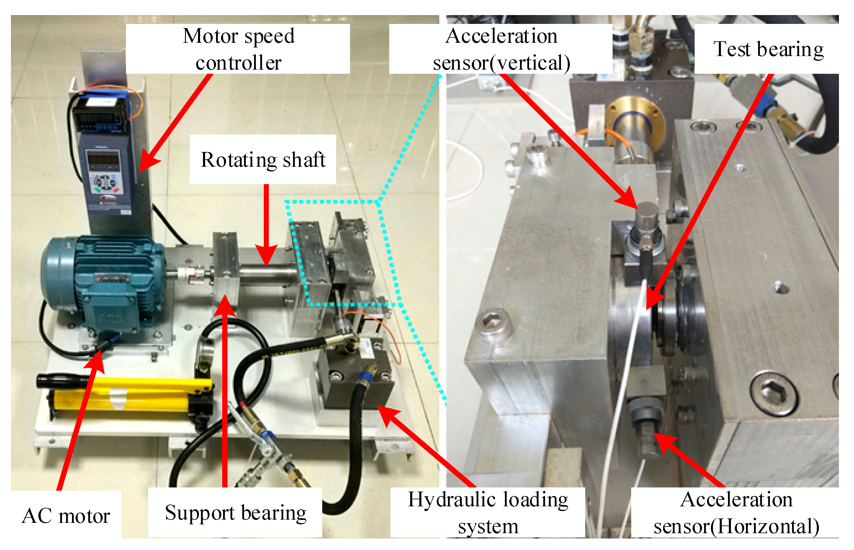
The test platform of XJTU consists of the rotating shaft, motor speed controller, support and test bearing, AC motor, and other parts; the test platform can be seen in Figure 12. Two unidirectional sensors were fixed in the vertical direction and horizontal direction of the test bearing by the magnetic base to obtain two sets of sensor data. The experimental bearing is LDK UER 204 rolling bearing, and the experiment has a 25.6 KHz sampling frequency. BPFO of the bearing is 115.62 Hz, BPFI is 184.38 Hz, and BSF is 144.66 Hz. The parameter information of the bearing is listed in Table 4.

Figure 12.
The experimental platform of XJTU.
Table 4.
LDK UER 204 rolling bearing parameters.
The selected fault types include five fault types: inner race, cage, outer race, composite fault of the inner and outer race (CFIO), and composite fault of the inner race, cage, and rolling body (CFICR). By taking 1024 data as a sample, a total of 2000 samples were selected from two sets of sensor data, and the sample number of each set of sensor data is 1000. In order to verify the method proposed in the paper, two samples were selected from two sets of sensor data, respectively, and the two selected samples were merged into a matrix with two rows and 1024 columns. That is, the new number of samples is 1000, of which 80% were used for training and 20% for tests. A detailed and specific description of the data used in the experiment of XJTU is given in Table 5.
Table 5.
Experimental datasets of XJTU.
4.2.2. Diagnostic Results and Analysis
First, the data were weighted by SAM, and then the weighted data were input into DWSC for DWC and PWC, as well as the subsequent convolution, BN and pooling, Sigmoid in turn, and classification.
The training and testing results of the proposed method on the XJTU datasets are shown in Figure 13. Figure 13a,b show the accuracy and loss changes of the training and testing datasets with epoch, respectively, and it can be observed that when the epoch is about 12, the model basically reaches convergence, and the changes of accuracy and loss tend to be basically stable, and the highest fault diagnosis accuracy rate is 100%. Figure 13c,d are the visualization results by t-SNE, Figure 13c is the visualization graph of the training result, and Figure 13d is the visualization graph of the test result. It can be clearly seen in Figure 13c,d that diverse fault types have an almost perfect separation degree. Figure 13e,f are the confusion matrix of the training and test results. It can be observed that the model proposed in the paper can identify and classify the five fault types perfectly and the recognition accuracy of each type of fault is 100%.
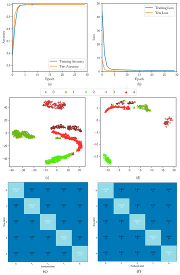
Figure 13.
Training and test results. (a,b) are the changes of accuracy and loss of the training and testing datasets with epoch, (c,d) are the visualization results of the training and testing results by t-SNE, (e,f) are the confusion matrix of the training and test results.
4.2.3. Diagnostic Results and Analysis
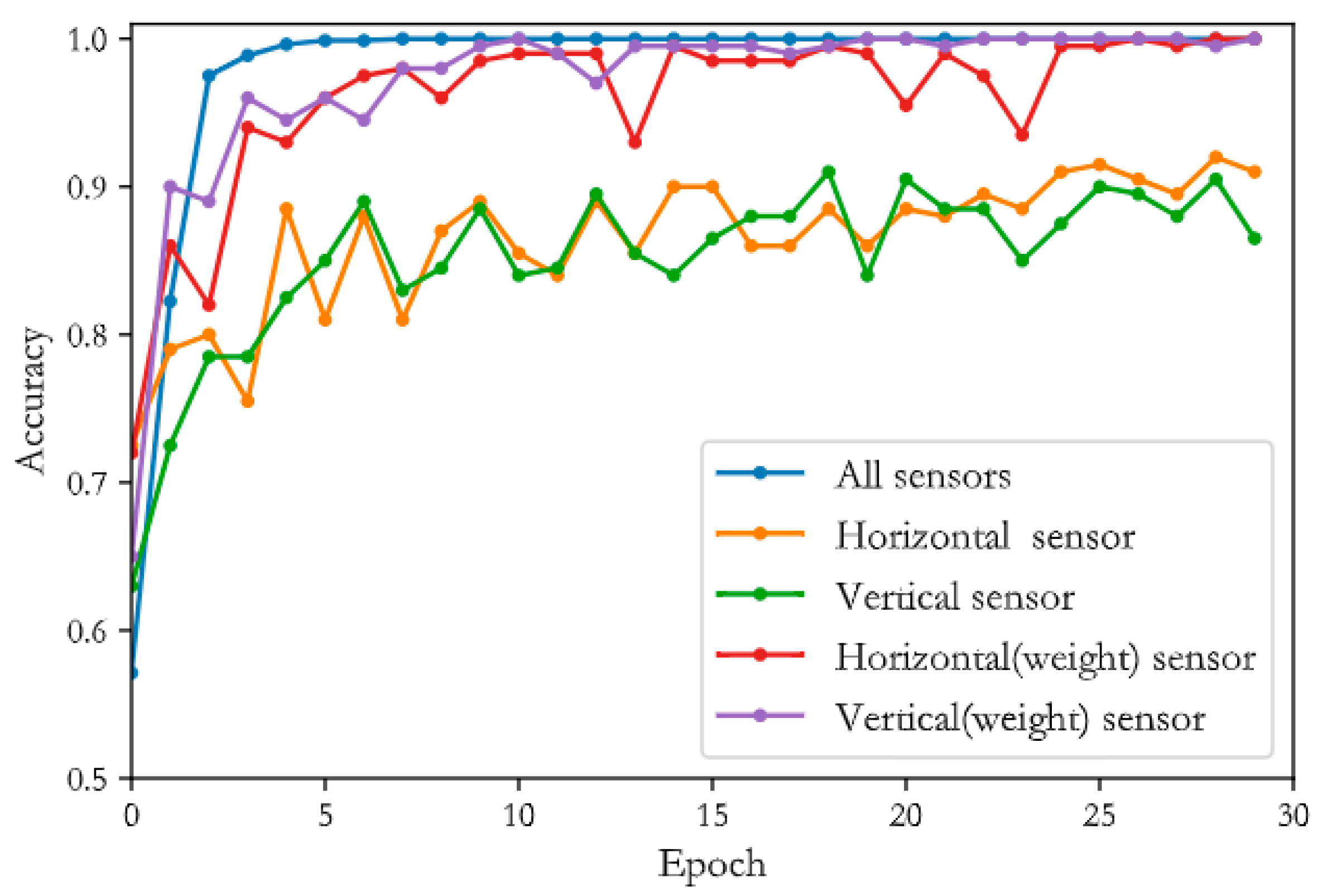
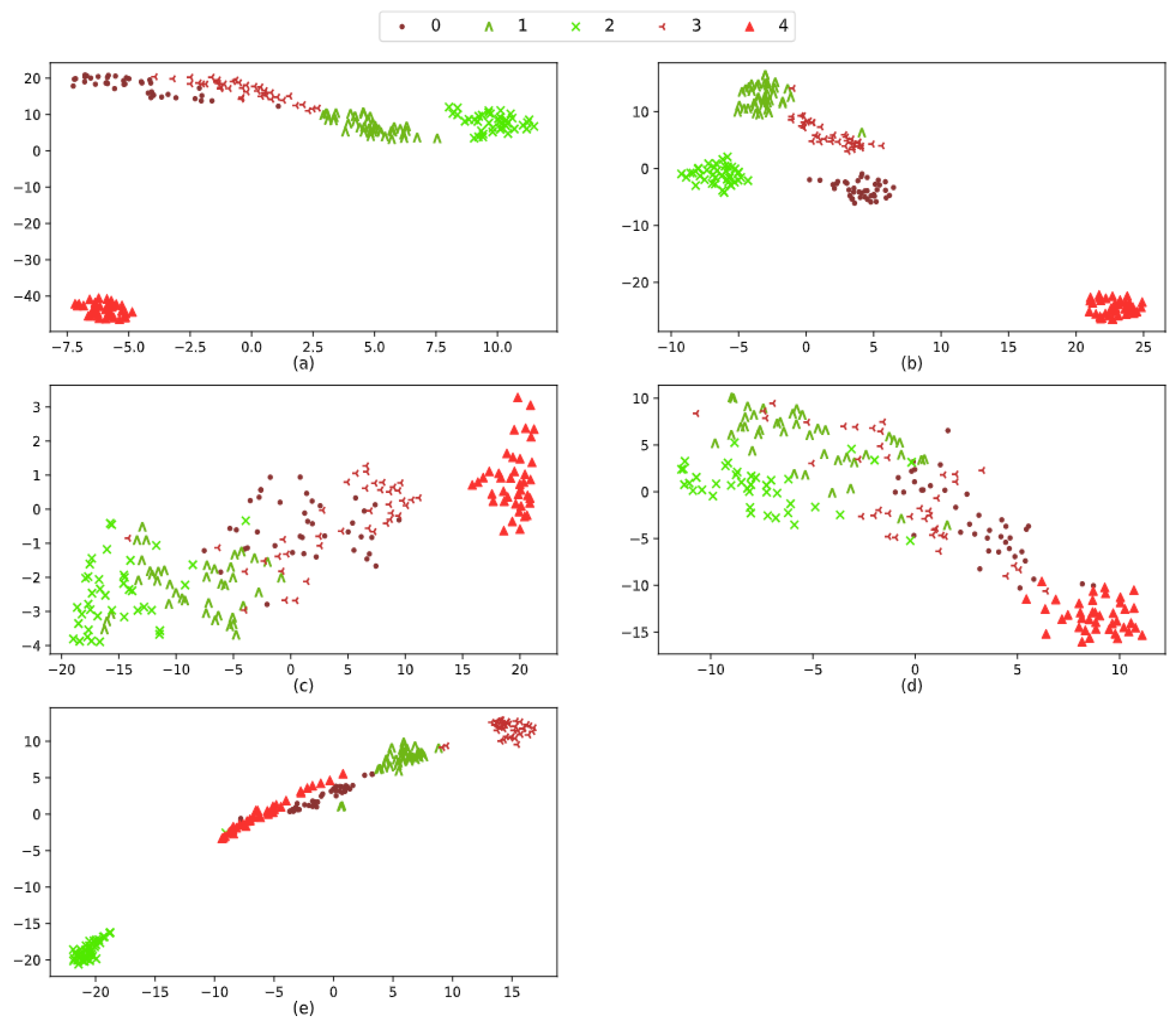
On the XJTU-bearing datasets, the performance of the MSDWF was also verified. That is, the multi-sensor and single sensor inputs are compared, and the weighted and unweighted data are compared. The results are shown in Figure 14. As can be seen in Figure 14, the weighted single sensor data have higher accuracy and faster convergence rate than the unweighted data, and the weighted data fusion of all sensors has the highest accuracy, fastest convergence rate, and best stability, which indicates the superior capacity and advantages of the method. The t-SNE visualization results of all the types of input are shown in Figure 15. Figure 15a,b are the t-SNE visualization results of the weighted data of the vertical sensor and horizontal sensor, respectively, which show a high degree of separation for each fault type, but a small part of the data is still mixed; Figure 15c,d are the t- SNE visualization results of the unweighted data respectively and the most of the data are mixed. Compared with the weighted data, there is no good recognition of various types of faults of the unweighted data. Figure 15e is the t-SNE visualization result of the weighted data of all sensors, and there is the highest degree of separation for each fault type.
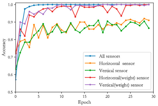
Figure 14.
Comparison of recognition accuracy between the different types input.
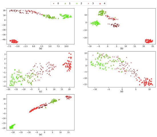
Figure 15.
Visualization results of t-SNE dimensionality reduction. (a,b) are the t-SNE visualization results of the weighted data of the vertical sensor and horizontal sensor respectively, (c,d) are the t-SNE visualization results of the unweighted data, (e) is the t-SNE visualization result of the weighted data of all sensors.
4.2.4. Comparison between Different Methods
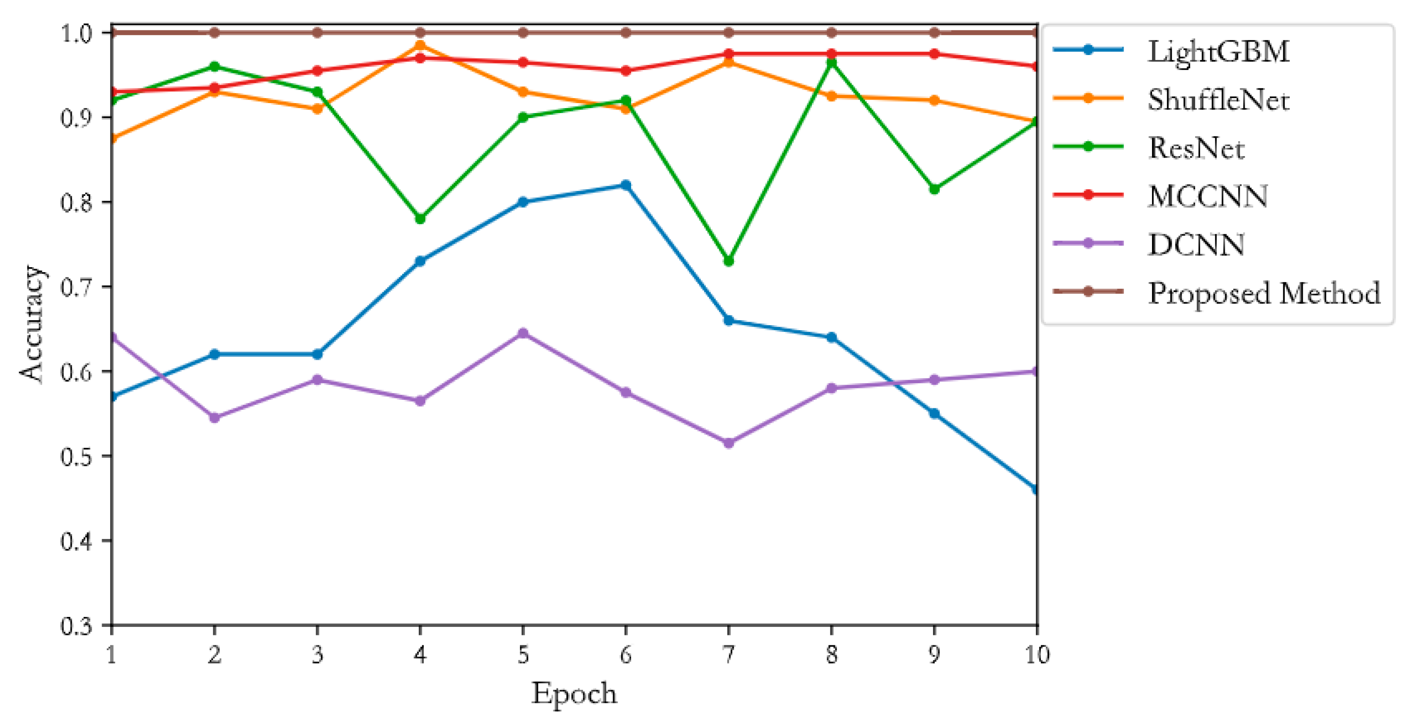
On the XJTU datasets, the proposed method was compared with Resnet, DCNN, ShuffleNet, MCCANN, and LightGBM. A total of ten comparison experiments were conducted, and comparative results can be seen in Figure 16. The average value and SD of classification results of all the methods are listed in Table 6. The average accuracy of the method proposed is 100%, followed by the MCCNN with an average accuracy of 95.95% and SD of 0.015. The accuracy of ShuffleNet and ResNet are 92.45% and 88.15%, with SD of 0.030 and 0.075, respectively. DCNN and LightGBM have the lowest accuracy, 58.45% and 64.70%, with SD of 0.037 and 0.106, respectively.

Figure 16.
Comparisons between the different fault diagnosis methods.
Table 6.
Average accuracy and SD of the different methods.
5. Conclusions and Future Work
Firstly, the weighting matrix is extracted from the data themselves of each sensor, and the weighted data are obtained by multiplying the raw data with the weighting matrix. The weak features in raw data are strengthened, and the effect of interference information caused by strong noise and variable working conditions on data features is weakened; the weighted data of all sensors are used as the input of DWSC to realize the decoupling of the channel and spatial correlation. In the proposed method, the data of multiple sensors are weighted and fused, taking into account the spatial and temporal information in the data. Through the comparative experiments between a different number of sensor inputs, the weighted and unweighted data, different fault diagnosis methods, and multiple datasets, the method based on MSDWF and DWSC shows superior performance, but it is worth pointing out that the training speed of the method needs further optimization and improvement.
Next, we will first consider optimizing this method to reduce the time it takes for each round of training. Secondly, the method will be tested in more complex and harsh environments and the performance in load adaptability so as to optimize and improve the method in a targeted manner. In addition, we will also test whether the accuracy can be further improved when using other types of sensors and different measuring points.
Author Contributions
Conceptualization, T.W. and X.X.; Data curation, X.X.; Formal analysis, T.Y. and H.X.; Methodology, T.W. and H.P.; Software, T.W. and X.Z.; Supervision, X.C.; Validation, H.P. and X.C.; Visualization, T.W.; Writing—original draft, T.W.; Writing—review & editing, T.W. and X.C. All authors have read and agreed to the published version of the manuscript.
Funding
This research received no external funding.
Conflicts of Interest
The authors declare no conflict of interest.
Nomenclatures
| MSDWF | Multi-sensor data weighted fusion |
| DWSC | Depth-wise separable convolutions |
| MCCNN | Multi-channel convolutional neural networks |
| BPFI | Ball pass frequency on inner race |
| BPFO | Ball pass frequency on outer race |
| BSF | Ball spin frequency |
| SAM | Self-attention method |
| PWC | Point-wise convolutions |
| DWC | Depth-wise convolutions |
| FCL | Fully connection layer |
| AM | Attention mechanism |
| CNN | Convolutional neural networks |
| MCCNN | Multi-channel convolutional neural networks |
| LightGBM | Light Gradient Bosting Machine |
| BN | Normalization batch |
| DL | Deep learning |
| NN | Neural networks |
| RMS | Root means square |
| SD | Standard deviation |
| t-SNE | t-distributed Stochastic Neighbor Embedding |
| KNNC | K-nearest neighbor classifier |
| PE | Permutation entropy |
| MPE | Multiscale permutation entropy |
| NLP | Natural language processing |
| DE | Drive end |
| FE | Fan end |
References
- Yan, X.; Jia, M. A novel optimized SVM classification algorithm with multi-domain feature and its application to fault diagnosis of rolling bearing. Neurocomputing 2018, 313, 47–64. [Google Scholar] [CrossRef]
- Heras, I.; Aguirrebeitia, J.; Abasolo, M.; Coria, I.; Escanciano, I. Load distribution and friction torque in four-point contact slewing bearings considering manufacturing errors and ring flexibility. Mech. Mach. Theory 2019, 137, 23–36. [Google Scholar] [CrossRef]
- Gao, S.; Chatterton, S.; Pennacchi, P.; Han, Q.; Chu, F. Skidding and cage whirling of angular contact ball bearings: Kinematic-hertzian contact-thermal-elasto-hydrodynamic model with thermal expansion and experimental validation. Mech. Syst. Signal Process. 2022, 166, 108427. [Google Scholar] [CrossRef]
- Ambrożkiewicz, B.; Syta, A.; Meier, N.; Litak, G.; Georgiadis, A. Radial internal clearance analysis in ball bearings. Eksploat. i Niezawodn. Maint. Reliab. 2021, 23, 42–54. [Google Scholar] [CrossRef]
- Cheng, Y.; Wang, S.; Chen, B.; Mei, G.; Zhang, W.; Peng, H.; Tian, G. An improved envelope spectrum via candidate fault frequency optimization-gram for bearing fault diagnosis. J. Sound Vib. 2022, 523, 116746. [Google Scholar] [CrossRef]
- Wang, Z.; Du, W.; Wang, J.; Zhou, J.; Han, X.; Zhang, Z.; Huang, L. Research and application of improved adaptive MOMEDA fault diagnosis method. Measurement 2019, 140, 63–75. [Google Scholar] [CrossRef]
- Guo, T.; Deng, Z. An improved EMD method based on the multi-objective optimization and its application to fault feature extraction of rolling bearing. Appl. Acoust. 2017, 127, 46–62. [Google Scholar] [CrossRef]
- Poongodi, C.; Hari, B.; Arunkumar, S. Vibration analysis of nylon gear box utilizing statistical method. Mater. Today Proc. 2020, 33, 3525–3531. [Google Scholar] [CrossRef]
- Wang, W.; Deng, L.; Zhao, R.; Wu, Y. Fault Feature Extraction Method of Rolling Bearing Based on Integrating KPCA and t-SNE. J. Vib. Eng. 2021, 34, 431–440. [Google Scholar]
- Wang, Z.; Zheng, L.; Du, W.; Cai, W.; Zhou, J.; Wang, J.; Han, X.; He, G. A Novel Method for Intelligent Fault Diagnosis of Bearing Based on Capsule Neural Network. Complexity 2019, 2019, 1–17. [Google Scholar] [CrossRef] [Green Version]
- Zhao, B.; Zhang, X.; Zhan, Z.; Wu, Q. Deep multi-scale adversarial network with attention: A novel domain adaptation method for intelligent fault diagnosis. J. Manuf. Syst. 2021, 59, 565–576. [Google Scholar] [CrossRef]
- Jiang, G.; He, H.; Yan, J.; Xie, P. Multiscale Convolutional Neural Networks for Fault Diagnosis of Wind Turbine Gearbox. IEEE Trans. Ind. Electron. 2019, 66, 3196–3207. [Google Scholar] [CrossRef]
- Zhao, B.; Zhang, X.; Li, H.; Yang, Z. Intelligent fault diagnosis of rolling bearings based on normalized CNN considering data imbalance and variable working conditions. Knowl. Based Syst. 2020, 199, 105971. [Google Scholar] [CrossRef]
- Zhao, M.; Zhong, S.; Fu, X.; Tang, B.; Pecht, M. Deep Residual Shrinkage Networks for Fault Diagnosis. IEEE Trans. Ind. Informatics 2020, 16, 4681–4690. [Google Scholar] [CrossRef]
- Liang, H.; Zhao, X. Rolling Bearing Fault Diagnosis Based on One-Dimensional Dilated Convolution Network with Residual Connection. IEEE Access 2021, 9, 31078–31091. [Google Scholar] [CrossRef]
- Hu, J.; Chen, Z.; Yang, M.; Zhang, R.; Cui, Y. A Multiscale Fusion Convolutional Neural Network for Plant Leaf Recognition. IEEE Signal Process. Lett. 2018, 25, 853–857. [Google Scholar] [CrossRef]
- Li, H.; Huang, J.; Ji, S. Bearing Fault Diagnosis with a Feature Fusion Method Based on an Ensemble Convolutional Neural Network and Deep Neural Network. Sensors 2019, 19, 2034. [Google Scholar] [CrossRef] [Green Version]
- Chen, Z.; Li, C.; Sanchez, R.-V. Gearbox Fault Identification and Classification with Convolutional Neural Networks. Shock Vib. 2015, 2015, 1–10. [Google Scholar] [CrossRef] [Green Version]
- Mao, W.; Ding, L.; Tian, S.; Liang, X. Online detection for bearing incipient fault based on deep transfer learning. Measurement 2020, 152, 107278. [Google Scholar] [CrossRef]
- Li, H.; Huang, J.; Yang, X.; Luo, J.; Zhang, L.; Pang, Y. Fault Diagnosis for Rotating Machinery Using Multiscale Permutation Entropy and Convolutional Neural Networks. Entropy 2020, 22, 851. [Google Scholar] [CrossRef]
- Jing, L.; Wang, T.; Zhao, M.; Wang, P. An Adaptive Multi-Sensor Data Fusion Method Based on Deep Convolutional Neural Networks for Fault Diagnosis of Planetary Gearbox. Sensors 2017, 17, 414. [Google Scholar] [CrossRef] [Green Version]
- Xia, M.; Li, T.; Xu, L.; Liu, L.; de Silva, C.W. Fault Diagnosis for Rotating Machinery Using Multiple Sensors and Convolutional Neural Networks. IEEE/ASME Trans. Mechatron. 2018, 23, 101–110. [Google Scholar] [CrossRef]
- Chen, Q.; Chen, Y.; Li, W.; Jia, Y. Multi-scale SE-Xception Clothing Image Classification. J. Zhejiang Univ. 2020, 54, 1727–1735. [Google Scholar]
- Luo, X.; Xia, X.; An, Y.; Chen, X. Chinese Clinical Entity Recognition Combined with Multi-head Self-Attention Mechanism and BiLSTM-CRF. J. Hunan Univ. 2021, 48, 45–55. [Google Scholar]
- Chollet, F. Xception: Deep learning with depthwise separable convolutions. In Proceedings of the 2017 IEEE Conference on Computer Vision and Pattern Recognition (CVPR), Honolulu, HI, USA, 21–26 July 2017. [Google Scholar]


Publisher’s Note: MDPI stays neutral with regard to jurisdictional claims in published maps and institutional affiliations. |
© 2022 by the authors. Licensee MDPI, Basel, Switzerland. This article is an open access article distributed under the terms and conditions of the Creative Commons Attribution (CC BY) license (https://creativecommons.org/licenses/by/4.0/).