Lateral Load Capacity and p-Multiplier of Group Piles with Asymmetrical Pile Cap under Seismic Load

Abstract

Earthquakes are a high-risk natural phenomenon in Indonesia, which is between three tectonic plates: the Eurasian, Pacific, and Indo–Australian plates. This study examines the response of bored piles with asymmetrical pile cap in the Auditorium Building of Brawijaya University to seismic loads, which is still rare to conduct this research. This study assessed based on 3D finite element-numerical approach, where lateral resistance and p-multiplier values compared on the effects of combination lateral loads, pile stiffness, and soil stiffness. The behavior of lateral resistance and deflection group piles with asymmetrical pile cap and single pile with square pile cap gives a good agreement. The side slope of the pile cap can increase the shear zone, increase the lateral resistance, and the most considerable lateral resistance to the lowest occurs in the horizontal direction, opposite the loading direction. In addition, the pile configuration that is not symmetrical gives an increasing p-multiplier value followed by an increasing deflection and the p-multiplier from the 3D finite element method was within the recommended range.

1. Introduction

The Indonesia Earthquake Hazard Map from the National Earthquake Study Library Team (2017) reveals that the country is between three main plates: the Eurasian Plate, the Indo–Australian Plate, and the Pacific Plate. The meeting of the large plates and several small plates or micro blocks causes regions in Indonesia to be prone to many earthquakes. As a result of tectonic processes, one earthquake source is the active subduction zone that spans the western to the eastern part of Indonesia. In addition, the remaining energy from the collision process between the plates will cause faults on land or in the sea in several islands and seas of Indonesia. The subduction zone in southern Java has only produced earthquakes with a magnitude of 7 in the last 20 years. However, a study showed possible earthquakes with a magnitude of 8 or 9 might occur in the subduction zone in the western part of Java [1].

Building structures in Indonesia are generally designed to withstand various environmental loads, especially earthquakes. Historically, structural safety has been measured by static variables requiring stiffness and strength. This may be due to earlier engineers’ lack of access to dynamics. Today, science shows that all objects that have stiffness and mass have dynamic behavior and many of these structures incorporate dynamic and cyclic loadings into the foundation.

The lateral capacity response is essential in the design of structures subjected to lateral loads. Understanding the behavior of piles under lateral loads is a complex problem because the soil−structure interactions that show the lateral load transfer mechanism depends on the soil layer and the pile itself. Pile deformation depends on lateral resistance, while lateral resistance is a function of the deformation itself. In addition, the p-multiplier is also used to see the soil−structure interaction. The p-multiplier can be directly calculated from the ratio or divided by the value of the lateral resistance calculated from the analysis of group piles and single piles.

In accepting the load, the pile cap is an essential structural element in the pile foundation because it functions to accept the load, which is then distributed to the foundation. In a plan, pile caps have various forms of modeling and always have different values in holding the load.

Several studies were conducted to determine the lateral load capacity and p-multiplier behavior of single pile and pile groups with symmetrical pile caps and configuration. Elhakim [2] performed three-dimensional finite element modeling to assess the response of laterally loaded piles embedded in the sand and confirmed the ability of finite element software to predict load-displacement relationships for pile groups of various configurations [2]. It is observed that the rear row of the pile has a more significant deflection than the front row of the pile for a certain distance. The load-deflection response for pile groups is softer than it is for single piles [2]. The study by Zhou et al. [3] adopted a two-stage analysis method to investigate the effect of lateral soil displacement on the fixed pile head. The study presents variations in the response (deflection, y) of piles with an undrained modulus of elasticity at a penetration depth of 12 m. When E_s increases from 2.5 MPa to 30 MPa, the deflection does not increase significantly, and the pile tip displacement decreases with increasing E_s [3]. Wang et al. [4] presented a numerical investigation to measure the effect of flexural stiffness on the load transfer curve (p-y curve) of a laterally loaded monopile in solid sand. As the flexural stiffness increases, the wedge failure mechanism regulates the pile behavior. However, due to the greater flexural stiffness, a larger soil zone is mobilized for the same deflection at the soil surface, and the depth of the effect of wedge failure also increases.

Lin and Lin [5] proposed a simple and practical method to evaluate the lateral behavior of pile groups based on a modified p-y method. The proposed method is verified with a three-dimensional finite element whose primary model is validated against pile group load testing. This shows that the resulting basic finite element model is good but slightly conservative for the front row compared to field test data. In other words, the three-dimensional finite element model exaggerates the shadow effect behind the top row, so the back row of the pile has a lower lateral resistance than the front row [5]. Cao et al. [6] discussed in detail the effects of rotational soil flow and additional resistance components on the lateral soil-pile behavior. Then, the validation was verified by centrifugal test and field test. The p-y API [7] method reduces stiffness and ultimate lateral resistance [6].

Zhu et al. [8] conducted an extensive parametric study to investigate the deformation behavior in more detail and the soil−pile interaction. A common constraint is adopted as an assumption in the design that the p-multiplier (p_m) remains constant throughout the load, and the entire pile depth range is critically examined. Overall observations show that the numerical model is reliable for the improvement of the soil-pile reaction while decreasing the overall flexural stiffness of the pile friction. The p_m parameter considers the pile group effect [8].

Since most pile groups used in practice are square and rectangular pile caps and pile configurations, very few research experiments have been carried out to observe the behavior of pile groups in misaligned pile caps and pile configurations. This research examined and compared the response or behavior of group bored piles with asymmetrical pile caps and single piles with square pile caps to seismic loads under equivalent static loads using three-dimensional finite element-based numerical and analytical methods. The output in this study is the distribution value of the lateral resistance and p-multiplier with different cases of combination lateral loads, soil stiffness, and pile stiffness. The results should help the behavioral determinants of the group pile’s foundation of the Auditorium Building at Brawijaya University to minimize the risk of failure in an earthquake disaster. In addition, a comparison between numerical and analytical methods is necessary to generate more accurate results; in this way, not only one result from one method but more than one result is obtained, so it can be seen which method is the best to use in confirmed cases in the field.

2. Literature Review

2.1. Piles under Seismic Load

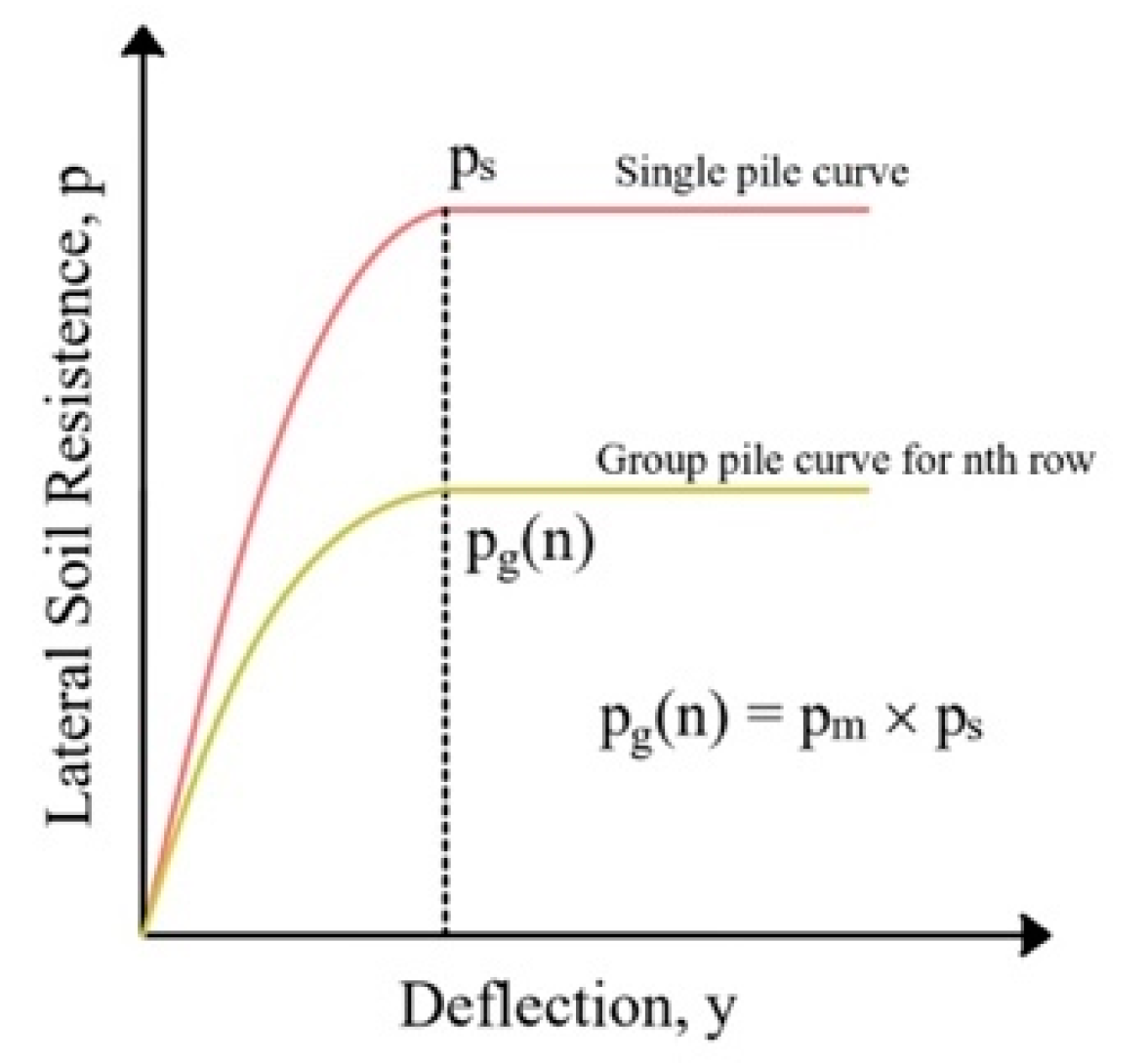
Pile failure due to seismic loading can be caused by excessive bending and shear forces resulting from inertial loading, kinematic loading, or both. It can also occur because of the large movements imposed on the pile by soil that has lost its shear stiffness [9]. The inertial forces increase the non-linear behavior of the soil and reduce the stiffness of the pile head. This effect increases the natural period of the structure-foundation system and alters the seismic spectral response. The kinematic forces arise from the pressure generated against the pile to ensure that the seismic displacement of the soil and pile is compatible at the contact points throughout the pile. Therefore, a notable seismic response can exert significant forces on the pile. Since inertial and kinematic forces can cause additional bending moments and shear forces in a pile, earthquakes can result in unacceptable permanent deformation [9].

Coulomb’s theory of active earth pressure can be extended by considering the forces generated by earthquakes. Figure 1 shows the lateral active pressure with the granular embankment. Note that the force acting on soil failure is essentially the same as that of failure under static conditions with the addition of k_hW and k_vW in the horizontal and vertical directions and can be defined as [10]:

$$\Delta {\mathrm{P}}_{\mathrm{ae}}={\mathrm{P}}_{\mathrm{ae}}-{\mathrm{P}}_{\mathrm{a}}$$

(1)

$${\mathrm{K}}_{\mathrm{ae}}=\frac{si{n}^2\left({\phi }^{\prime }+\beta -{\theta }^{\prime }\right)}{cos{\theta }^{\prime }si{n}^2\beta sin\left(\beta -{\theta }^{\prime }-{\delta }^{\prime }\right)\left[1+\sqrt{\frac{sin\left({\phi }^{\prime }+{\delta }^{\prime }\right)sin\left({\phi }^{\prime }-{\theta }^{\prime }-\alpha \right)}{\sin \left(\beta -{\delta }^{\prime }-{\theta }^{\prime }\right)sin\left(\alpha +\beta \right)}}\right]} ; \mathsf{\theta }\text{’}=\tan {-}^1\left[\frac{k_h}{\left(1-k_v\right)}\right]$$

(2)

$$\begin{gathered} {\mathrm{k}}_{\mathrm{h}}=\frac{horizontal earthquake acceleration component}{acceleration due to gravity, g}; \\ {\mathrm{k}}_{\mathrm{v}}=\frac{vertical earthquake acceleration component}{acceleration due to gravity, g} \end{gathered}$$

(3)

where P_ae = active force per unit length of the wall in earthquake conditions, P_a = active force per unit length of the wall in static conditions, K_ae = coefficient of active earth pressure in earthquake conditions, and k_h, k_v = coefficient of horizontal and vertical ground acceleration in earthquake conditions.

If a structure is subjected to seismic loads, the following load combinations must be considered together with the base load combination. The essential combination for the allowable stress design is [11]:

(1.0 + 0.14S_DS) D + 0.7E_h

(4)

(1.0 + 0.105S_DS) + 0.525E_h + 0.75L

(5)

(0.6 − 0.14S_DS) D + 0.7E_h

(6)

where S_DS = design acceleration spectral response parameter in a short period (2/3 × F_aS_s), E_h = horizontal seismic load effect, L = live load, and F_a = site coefficient (taken based on the value of the maximum seismic acceleration spectral response parameter that is considered risk-targeted (MCE_R) is mapped in the short period, S_s, and the 1 s period, S₁, in SNI 1726 [11]).

2.2. p-Multiplier

Zhou and Tokimatsu [12] stated that the behavior of piles in groups that received lateral loads were different from that of a single pile. The lateral load borne by each pile in the group varies according to its position. This effect is commonly referred to as the pile group effect. To account for the loss of soil resistance in the pile design, Brown et al. [13] further proposed a p-multiplier approach. As shown in Figure 2, the p-multiplier or p_m is used to modify a single pile lateral soil spring to obtain pile springs in a group. Usually, the p-multiplier is constant in the same row.

The p-multiplier can be calculated from the p-y curve by dividing the single pile soil resistance by the pile group. The p-y curve is the soil reaction to the pile (p), which is related to the pile deflection (y) through a non-linear load-deflection curve. The p-y formulation based on API [7] can be calculated as follows:

$$\frac{p}{p_{u}D}=\tanh a{\left(\frac{y}{D}\right)}^b$$

(7)

where $p$ = lateral soil resistance per unit length of the pile, y = pile deflection, and p_u = lateral bearing capacity.

New development of the p-y method can be used to describe better soil-pile behavior based on API [7], as cited in Cao et al. [6]:

$$\begin{array}{c}\mathrm{a}=8.62{\left(\frac{L_p}{D}\right)}^{-0.18}\hfill \\ \mathrm{b}=0.5\hfill \\ {\mathrm{L}}_{\mathrm{p}}=\mathrm{pile\; depth}\hfill \end{array}$$

(8)

Based on full-scale testing, Rollins et al. in FEMA p-751 [14] recommended a p-multiplier, p_m, where D is the diameter or width of the pile and s is the center-to-center distance between the piles in the direction of loading.

First (leading) row piles:

$${\mathrm{p}}_{\mathrm{m}}=0.26\ln \left(\frac{\mathrm{s}}{\mathrm{D}}\right)+0.5\text{≤}1.0$$

(9)

Second row piles:

$${\mathrm{p}}_{\mathrm{m}}=0.52\ln \left(\frac{\mathrm{s}}{\mathrm{D}}\right)\text{≤}1.0$$

(10)

Third or higher row piles:

$${\mathrm{p}}_{\mathrm{m}}=0.60\ln \left(\frac{\mathrm{s}}{\mathrm{D}}\right)-0.25\text{≤}1.0$$

(11)

Reese and Impe [15] formulated the prediction equation by adjusting the curve to the data, representing efficiency with pile distance. There is no distinction for soil type, pile diameter, or penetration.

Leading piles:

$${\mathrm{p}}_{\mathrm{m}}=0.7{\left(\frac{\mathrm{s}}{\mathrm{D}}\right)}^{0.26}$$

(12)

Trailing piles:

$${\mathrm{p}}_{\mathrm{m}}=0.38{\left(\frac{\mathrm{s}}{\mathrm{D}}\right)}^{0.38}$$

(13)

where p_m = p-multiplier, s = distance between piles, and D = diameter of the pile.

The p-multiplier (p_m) is taken from the center-to-center distance of the pile in the loading direction group, expressed in multiples of the pile diameter (D). The calculation of group effects based on the American Association of State Highway and Transportation Officials [16] is shown in

Table 1. p-multiplier according to AASHTO [16].

Pile Space	p-Multiplier, pm
	Row 1	Row 2	Row 3 and Upper
3D	0.8	0.4	0.3
5D	1	0.85	0.7

.

The p-multiplier depends on the pile spacing and row number according to the direction of loading. In order to assign the p_m value to the other pile spacing values, interpolation between values must be carried out [16].

2.3. Soil Stiffness

Measurement of soil stiffness directly in the field can minimize disturbance. The modulus measured in the field corresponds to a very small strain. The in-situ technique is based on measuring the velocity of the stress wave through the ground. The pore fluid response in saturated soil dominates the P-wave or compression wave. As a result, most measured waves are S-waves or shear waves. If the shear wave velocity through the soil deposit is specified as V_s, then the shear modulus (small strain) G_max is given as [17]:

G_max = ρ V_s²

(14)

$${\mathrm{G}}_{\max }=\frac{\mathsf{\gamma }}{\mathrm{g}}{{\mathrm{V}}_{\mathrm{s}}}^2$$

(15)

where, ρ = soil density mass, γ = weight of soil, G_max = shear modulus of seismic conditions, and V_s = shear wave velocity.

From the basic theory of elasticity, the modulus of elasticity (E_s) can be related to the shear modulus of seismic conditions (G_max) as follows [18]:

E_s = 2 (1 + v) G_max

(16)

where v = poisson’s ratio.

Researchers from various countries have proposed empirical correlations between soil V_s values and N-SPT [19,20,21,22]. According to SPT implementation standards, N-SPT is the number of blows required to obtain the last 30 cm of sample tube penetration from a total of 45 cm at each test step. Sample penetration is obtained from a hammer weighing 63.5 kg dropping from a constant free fall height (76 cm) to the anvil mounted on the drill post. The test results cannot be separated from the influence of equipment features and procedures, including the energy content of the hammer. Some of these empirical equations are based on the number of SPT blows with corrected energy (N₆₀), and the number of SPT blows corrected with energy and stress (overburden) (N₁)₆₀ [20,21].

The main characteristics of each study were the location, soil type, soil stiffness, geological age (if available), type of function used for SPT-V_s correlation, constant regression coefficient, number of data pairs, and R² value. In general, the most suitable function for SPT-V_s data regression is a function as shown in the following equation [21]:

V_s = A × N₆₀^B

(17)

where A and B = constant regression coefficient, N₆₀ = corrected N-SPT with energy, and V_s = wave shear velocity at the same depth at which the N-SPT value is measured.

Hasancebi and Ulusay in Hammam and Eliwa [22] stated that the equation for all types of soils, soft soils, and sands based on the number of blows of N-SPT corrected with energy (N₆₀) applies to indirect estimates of V_s as follows:

All soils = 104.79 × N₆₀^0.26

(18)

Although it is preferable to determine shear wave velocities directly from field tests, measurement of V_s is often not economical at all locations [23]. The correlation equation developed between V_s (m/s) and N-SPT corrected with energy and suitable for all soils by simple regression analysis based on Maheswari et al. [23] are as follows [20]:

All soils = 90.75 × N₆₀^0.304

(19)

Sand = 96.29 × N₆₀^0.266

(20)

Tsimbaos and Sabatakakis [24] conducted a study using a relational database consisting of 416 V_s-N. The data evaluated refers to soft−hard clay soils (classified as CH, CL, and SC according to USCS), loose−very dense silty sand (SM), and loose−very dense silt (ML). Regression analysis was used to define the relationship between V_s and penetration resistance. A regression procedure is used to adjust the curve through the points to minimize the squared deviation of the measured points. The relevant equations define the curves in the two-variable spaces, and the coefficient of determination (R²) value is calculated.

All soils = 105.7 × N₆₀^0.327

(21)

Sand = 79.7 × N₆₀^0.365

(22)

3. Methodology

The lateral resistance of the group pile and the single pile was analyzed using a 3D finite element-based numerical method. The p-multiplier values were compared with analytical methods from FEMA P-751 [14] in Equations (9)–(11), Reese and Impe [15] in Equations (12) and (13), and AASHTO [16] in Table 1, as well as the numerical method by dividing the result of the load value of a single pile by the value of the group piles.

This study seeks to understand and compare the behavior of group piles with asymmetrical pile caps and single piles with square pile caps on the distribution of lateral load capacity and the p-multiplier. This study also examines their behaviors at various combination lateral loads (P), pile stiffness (E_p), and pile stiffness (E_s).

The combination lateral loads consist of lateral earth pressure on semi-basement walls, and earthquake load was taken based on the value of the MCE_R acceleration spectral response parameter by static equivalent method and mapped for a short period (S_s) and 1.0 s period (S₁); S_s = 0.80 and S₁ = 0.40, S_s = 1.00 and S₁ = 0.40, S_s = 1.20 and S₁ = 0.50. Soil stiffness was compared using the value of shear wave velocity (V_s) derived from N-SPT data (

Table 2. N₆₀ and V_s value derived from SPT data.

Parameters	Methods	Unit	MH	MH	SC-SM	SC-SM	CL
Depth		M	0.00–5.50	5.50–8.50	8.50–11.50	11.50–14.50	14.50–17.50
$\overline{\mathrm{N}}$60			12	11	14	28	34
Vs	Maheswari et al., 2010 [23]	m/s	176.67	172.18	194.68	233.75	243.14
	Hasancebi and Ulusuay, 2006 in Hammam and Eliwa [22]		204.80	200.34	208.53	249.35	269.12
	Tsimbaos and Sabatakakis, 2011 [24]		237.39	230.90	209.41	269.15	334.70
Parameters	Methods	Unit	MH	SM	SM	MH	CL-ML
Depth		M	17.50–20.00	20.00–23.50	23.50–26.50	26.50–29.50	29.50–30.00
$\overline{\mathrm{N}}$60			44	68	55	54	55
Vs	Maheswari et al., 2010 [23]	m/s	263.66	296.06	279.39	279.36	241.78
	Hasancebi and Ulusuay, 2006 in Hammam and Eliwa [22]		288.43	314.14	296.83	303.06	305.09
	Tsimbaos and Sabatakakis, 2011 [24]		365.18	372.23	343.76	388.62	456.36

) values using methods from Hasancebi and Ulusuay in Hammam and Eliwa [22] in Equation (18), Maheswari et al. [23] in Equations (19) and (20), and Tsimbaos and Sabatakakis [24] in Equations (21) and (22), while the pile stiffness was appealed to the value of the concrete quality of K-250, K-350, and K-450.

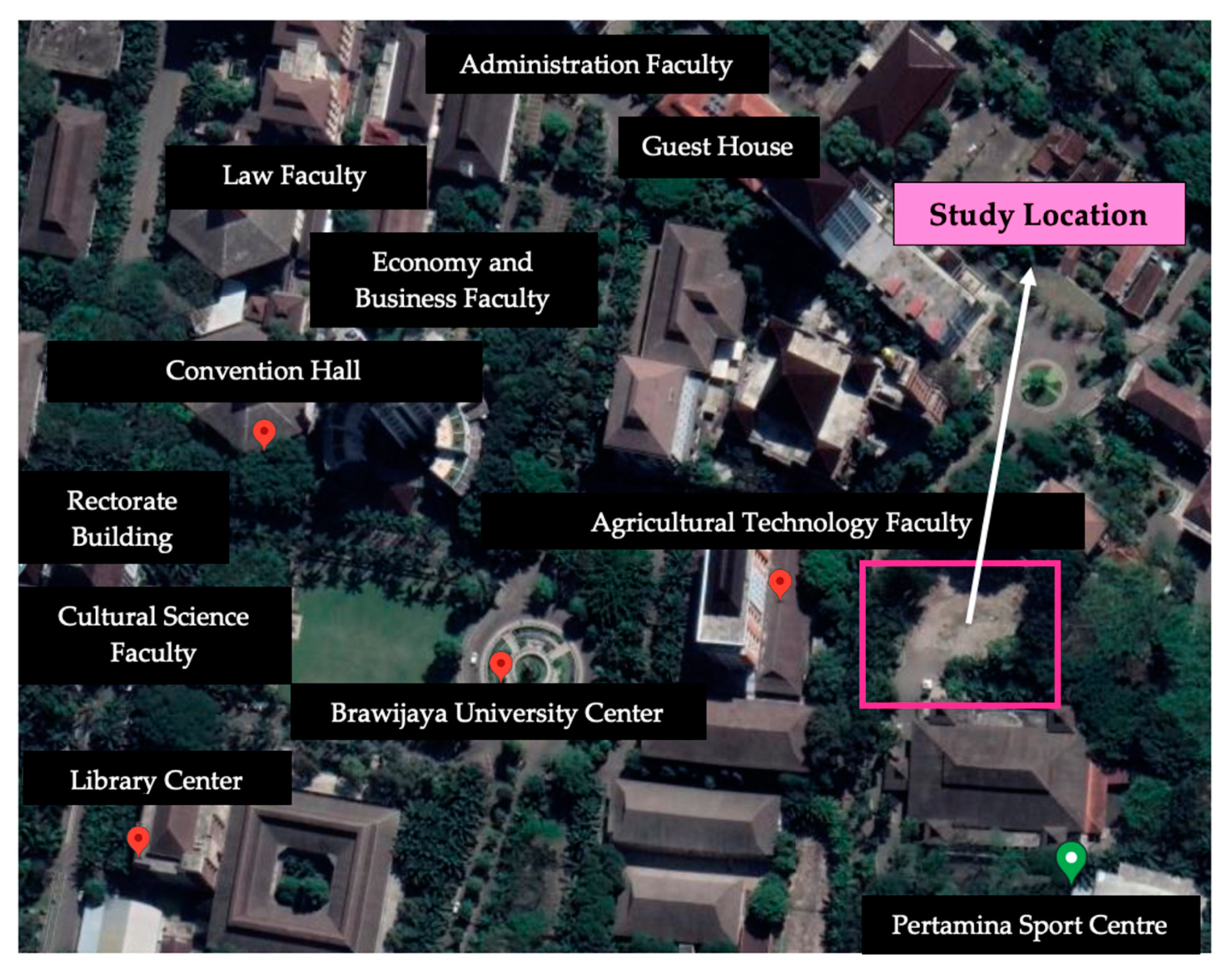
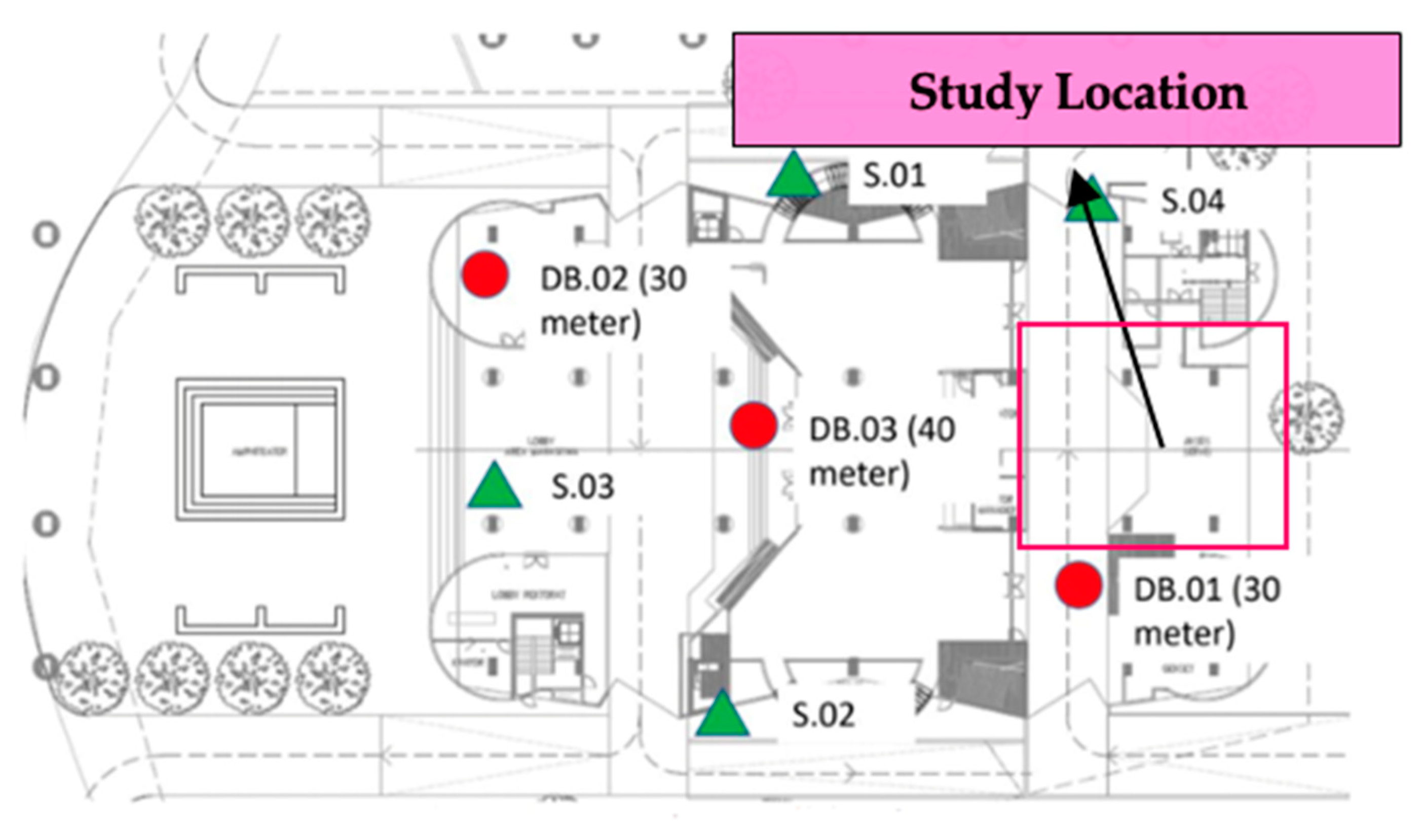
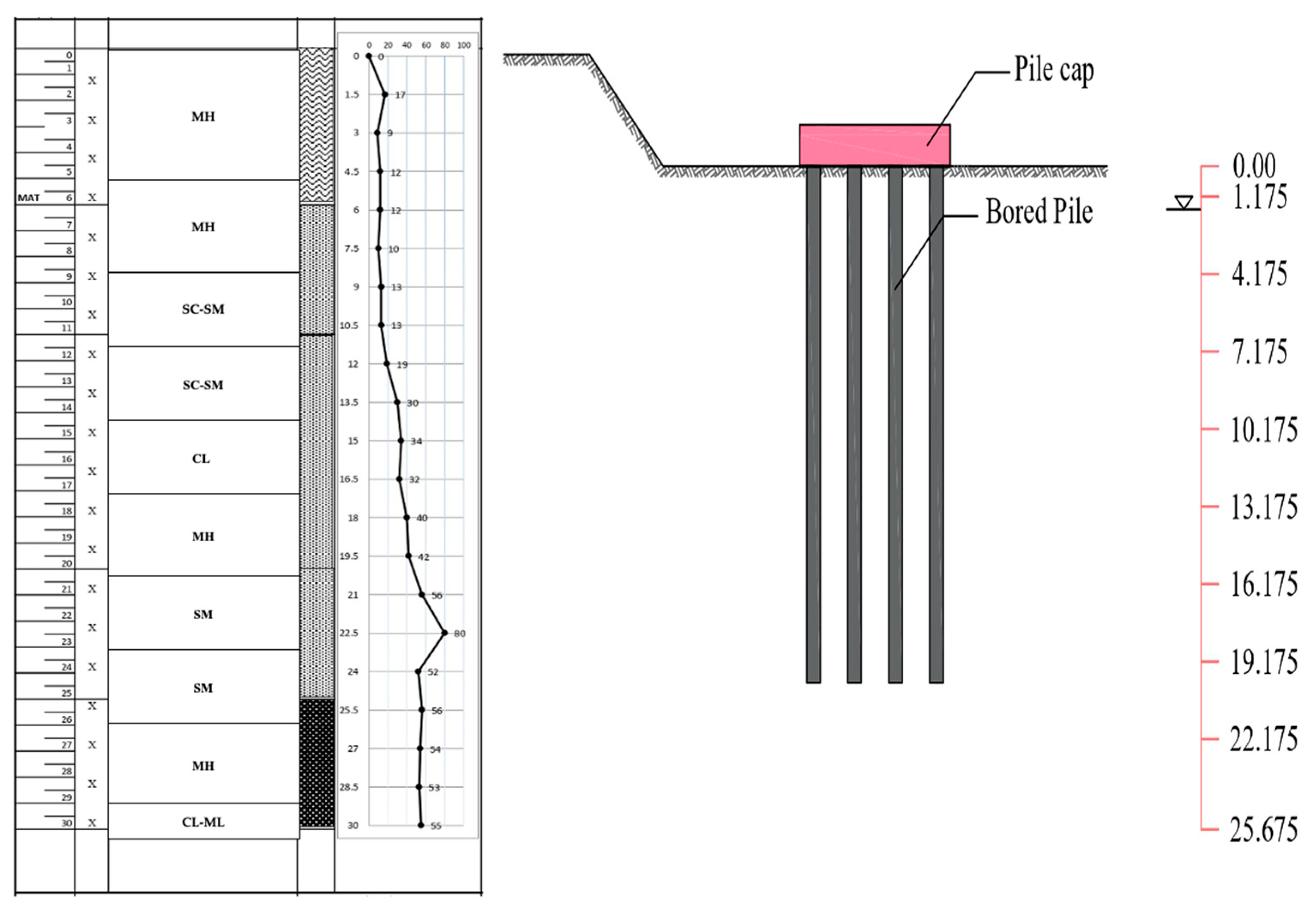
3.1. Site Characteristics

The study site is located in the center of Malang City, right inside the area of Brawijaya University at coordinates 7°57′08″ S, 112°36′56″ E (Figure 3). This building is used as a meeting hall and educational facility for the campus area. The 2nd floor consists of a large meeting room, while the balcony is on the 4th and 5th floors. The substructure planned to use a reinforced concrete bored pile foundation. A soil investigation was carried out by the Laboratory of Soil Mechanics and Geology, Faculty of Engineering, Brawijaya University, from three boring points and four 2.5-ton cone penetration points. The bored piles studied are located near DB point 01 (Figure 4).

Based on the SPT elevation, the bored pile elevation (Figure 5) was initiated 4.325 m below ground level. However, in the finite element modeling, the elevation was assumed to be 0.00 m. With groundwater elevation, the SPT elevation was 6.00 m below ground level and was assumed to be −1.675 m in the modeling.

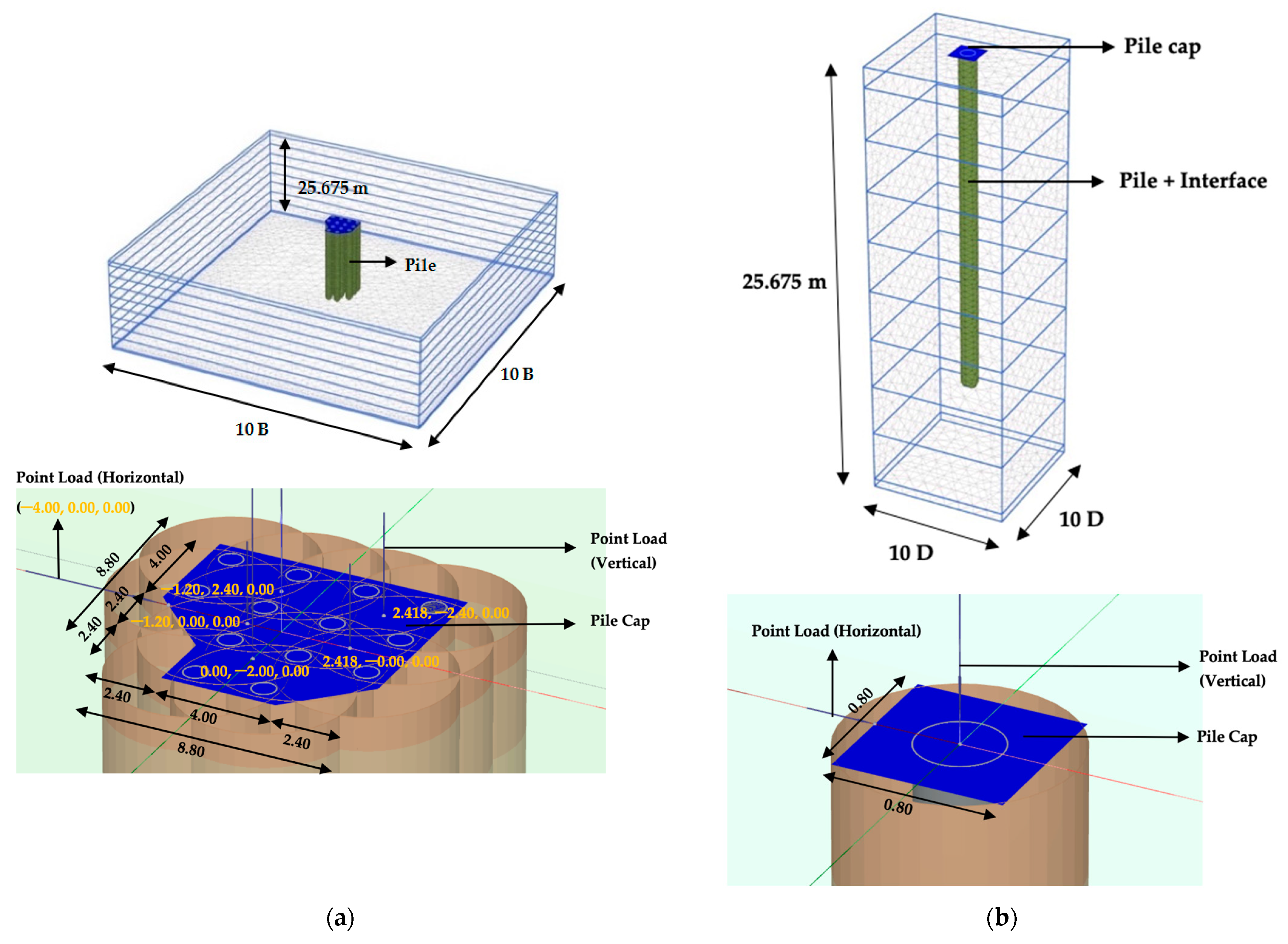
3.2. Finite Element Method

The 3D modeling of the single pile and group pile used tetrahedral meshing with 15-node elements. For the single pile, the values of x-max, x-min, y-max, and y-min are obtained as 5 D from the global coordinate. The x-max and y-max are 4 m and the x-min and y-min are −4 m. For the group pile, the distance from the tip of the pile to the end of the mesh, namely x-max, x-min, y-max, and y-min, was taken by 5 B (B = pile cap width) from the global coordinates so that the x-max and y-max values were 44 m, while x-min and y-min values were −44 m. The default units were chosen, with m (meters) for length and kN (kilo Newtons) for force. The modeled pile is 20 m long. Since the modeling geometry is volume pile, the pile was described as the full diameter (0.80 m) with the distance between the piles being 2.4 m in the group pile (Figure 6). The pile cap is square-shaped for the single pile and asymmetrical for the group pile. Pile caps are considered rigid bodies to ensure equal movement of all pile heads [25].

For software input, in the case of the single pile, the axial and lateral loads are point loads with a load value equal to the allowable axial bearing capacity and combination lateral loads. For the case of group piles, the input value is the total combination lateral loads from static equivalent earthquake loads and soil pressure on the semi-basement wall for lateral loading. One pile cap consists of five columns. Thus, there were five-point vertical loads, and each point load’s coordinates were adjusted from the detailed pile cap drawing (Figure 6a). The interface in the soil-structure interaction is weaker and more flexible than the surrounding soil. Therefore, the R_inter value should be less than 1 [26].

The default standard pinch boundary conditions were used, in which the standard pinch limit means that the x-min, x-max, y-min, and y-max were normally fixed, z-min was fully fixed, and z-max was free for 3D analysis.

Stage construction consists of four phases: the initial phase, pile construction, plate construction, and loading phase. In the initial phase, all structural geometries are inactive. In the pile construction phase, pile materials and interfaces are activated. The plate construction phase activates the plate material, while the whole pile geometry and point loads are activated in the loading phase. The axial load is activated when analyzing the lateral load.

3.3. Loads and Material Characteristics

The combination lateral loads (P) consist of equivalent static earthquake loads based on SNI 1726 [11], and lateral earth pressure on semi-basement walls according to Das [10] using Columb’s theory in Equation (1). The earthquake load by the static equivalent method was taken based on the amplification factor for a short period (S_s) and 1.0 s period (S₁) at Malang city, Indonesia (Figure 7) from the Indonesian Earthquake Zone Map, where the S_s value occurs at 0.80–1.00 g (red color) and the S₁ value occurs at 0.30–0.50 g (yellow color). Therefore, the amplification factor for a short period (S_s) and 1.0 s period (S₁) in this research was taken as S_s = 0.80 and S₁ = 0.40 for condition 1, S_s = 0.90 and S₁ = 0.40 for condition 2, and S_s = 1.00 and S₁ = 0.50 for condition 3. The amplification factor was used to determine the MCE_R acceleration spectral response and design spectral acceleration parameters. The combination lateral load values of the group pile (P_G) were 7051.887 kN for condition 1 (P_G1), 8973.120 kN for condition 2 (P_G2), and 10,690.011 kN for condition 3 (P_G3). At once, the combination lateral load values of the single piles (P_S) are calculated from the group pile divided by the number of piles; these values are 542.453 kN for condition 1 (P_S1), 690.240 kN for condition 2 (P_S2), and 822.309 kN for condition 3 (P_S3). The input load used in condition 3 was used in the analysis of the effects of pile stiffness and soil stiffness. The axial input load for a single pile is 956.495 kN, which is taken from the axial ultimate bearing capacity. For the case of the group piles, they consist of 5 axial loads generated based on column reactions due to service loads, where the first axial load with coordinates (0.00, −2.00, 0.00) is 3088.864 kN, the second axial load with coordinates (−1.20, 0.00, 0.00) is 949.60 kN, the third axial load with coordinates (2.418, 0.00, 0.00) is 970.236 kN, the fourth axial load with coordinates (−1.20, 2.40, 0.00) is 1297.65 kN, and the fifth axial load with coordinates (2.418, −2.40, 0.00) is 1190.500 kN.

Poulos and Davis [27] proposed a method for classifying piles into different categories based on the flexibility factor, K_r (K_r = E_pI_p/E_sL_p⁴). Where, I_p is the inertia moment of the pile and L_p is the pile length. The classification of the bored pile at Brawijaya University consists of a flexibility factor of 44 $\times$ 10⁻⁵ from E_p1 = 20.75 MPa, 52 $\times$ 10⁻⁵ from E_p2 = 29.05 MPa, and 59 $\times$ 10⁻⁵ from E_p3 = 37.35 MPa with E_s from Tsimbaos and Sabatakakis [24] at 20.00 m depth. From this value, based on Li et al., 2014 [28], the piles are categorized as very flexible piles with a flexibility factor of 10⁻⁵.

There were three values of modulus of elasticity used in this study calculated by Equations (16)–(22) (

Table 3. Modulus of elasticity.

Parameters	Symbol	Unit	MH	MH	SC-SM	SC-SM	CL
Depth		M	0.00–5.50	5.50–8.50	8.50–11.50	11.50–14.50	14.50–17.50
Shear Modulus	Gmax1	kN/m2	31,512.89	30,168.81	54,463.84	58,647.40	62,843.00
	Gmax2	kN/m2	42,346.40	40,843.44	62,487.42	66,734.39	76,989.80
	Gmax3	kN/m2	56,897.20	54,258.68	63,015.42	77,752.24	119,082.54
Modulus of Elasticity	Es1	kN/m2	80,257.83	76,107.67	141,750.84	157,208.03	172,158.08
	Es2	kN/m2	107,848.87	103,036.85	162,633.48	178,885.72	210,913.15
	Es3	kN/m2	144,907.24	136,879.86	164,007.69	208,419.75	326,226.01
Parameters	Symbol	Unit	MH	SM	SM	MH	CL-ML
Depth		M	17.50–20.00	20.00–23.50	23.50–26.50	26.50–29.50	29.50–30.00
Shear Modulus	Gmax1	kN/m2	71,347.32	137,818.78	132,539.58	81,007.64	66,740.49
	Gmax2	kN/m2	85,382.60	155,159.96	149,607.27	95,333.66	106,266.07
	Gmax3	kN/m2	136,865.04	217,852.44	200,658.77	156,762.39	237,768.36
Modulus of Elasticity	Es1	kN/m2	199,772.48	385,892.57	371,110.81	226,821.40	186,873.38
	Es2	kN/m2	239,071.29	434,447.88	418,900.34	266,934.24	297,544.98
	Es3	kN/m2	383,222.10	609,986.82	561,844.55	438,934.70	665,751.40

), where E_s1 was the value of the young modulus using the shear wave velocity value approach from Maheswari et al. [23] and E_s2 used the modulus based on Hasancebi and Ulusuay in Hammam and Eliwa [22]. Meanwhile, E₃ was based on Tsimbaos and Sabatakakis [24], where the V_s values used to determine the value of G_max in Equation (14), in which the value of $\overline{\mathrm{N}}$ was in the range of 15 to 50 and V_s was in the range of 175 to 350.

The Mohr–Coulomb model was used in finite element modeling (

Table 4. Soil characteristics.

Parameters	Symbol	Unit	MH	MH	SC-SM	SC-SM	CL
Depth			0.00–5.50	5.50–8.50	8.50–11.50	11.50–14.50	14.50–17.50
Material model			Mohr–Coulomb	Mohr–Coulumb	Mohr–Coulumb	Mohr–Coulumb	Mohr–Coulumb
Behavior type			Undrained	Undrained	Drained	Drained	Undrained
Density above water table	γunsat	kN/m3	9.901	9.980	14.092	10.526	10.424
Density below water table	γsat	kN/m3	15.532	15.417	18.159	16.092	15.918
Effective density	γ′	kN/m3	5.725	5.61	8.352	6.285	6.111
Poisson ratio	v		0.273	0.261	0.301	0.340	0.370
Cohesion	c	kN/m2	35.598	17.162	4.021	1.177	15.789
Friction angle	φ	o	30.45	25.62	44.26	44.29	31.75
Rinter			0.901	1.00	0.543	0.543	0.856
Parameters	Symbol	Unit	MH	SM	SM	MH	CL-ML
Depth		M	17.50–20.00	20.00–23.50	23.50–26.50	26.50–29.50	29.50–30.00
Material model			Mohr–Coulumb	Mohr–Coulumb	Mohr–Coulumb	Mohr–Coulumb	Mohr–Coulumb
Behavior type			Undrained	Drained	Drained	Undrained	Undrained
Density above water table	γunsat	kN/m3	10.065	15.419	16.652	10.179	11.196
Density below water table	γsat	kN/m3	15.614	19.191	20.252	16.288	16.349
Effective density	γ’	kN/m3	5.807	9.384	10.445	6.482	6.543
Poisson ratio	V		0.4	0.4	0.4	0.4	0.4
Cohesion	C	kN/m2	19.221	9.12	0.588	21.673	3.825
Friction angle	φ	o	18.8	40.9	51.75	17.19	40.9
Rinter			1.00	0.611	0.417	1.00	0.611

). Linear elastic perfectly-plastic is a first-order model that includes only the number of features exhibited by the behavior of the soil. In general, the effective stress uses the Mohr–Coulomb failure criteria with the effective strength parameters of φ′and c′ [29].

The interaction between the structural elements and the soil was modeled through the interface. The interface element was used to reduce the friction between the structural element and the soil (R_inter), which has a value between 0.01 and 1.0 (Table 4). The lower limit value of 0.01 indicates no friction between the structural elements and the soil. The upper limit value of 1.0 means that the structural element and the soil are in contact and cannot slip over each other (rigid) [30]. R_inter is taken by dividing the friction angle in the concrete pile by the soil friction angle at each depth. The concrete friction angle was approximated at 27.90° based on direct shear testing by Ilori et al. [31] to investigate the interaction between the soil and concrete in-situ concerning friction.

4. Results and Discussion

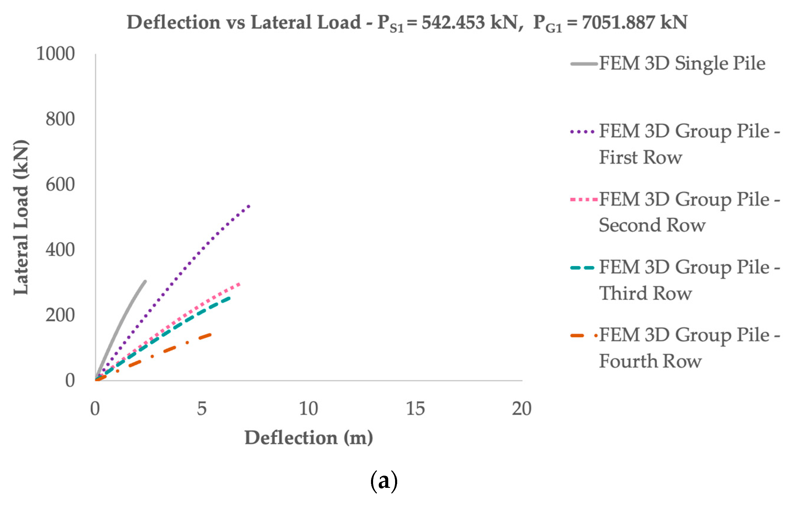
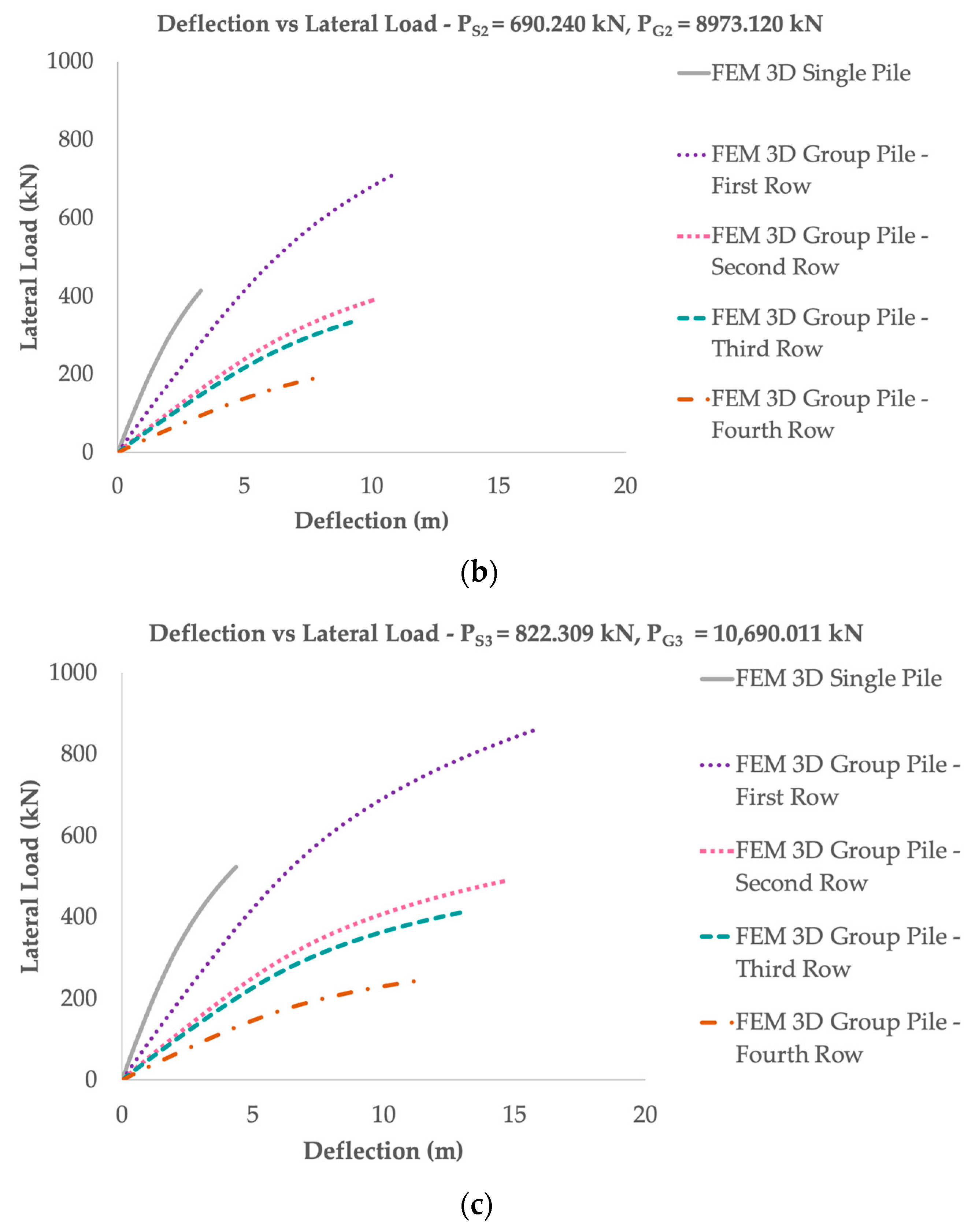
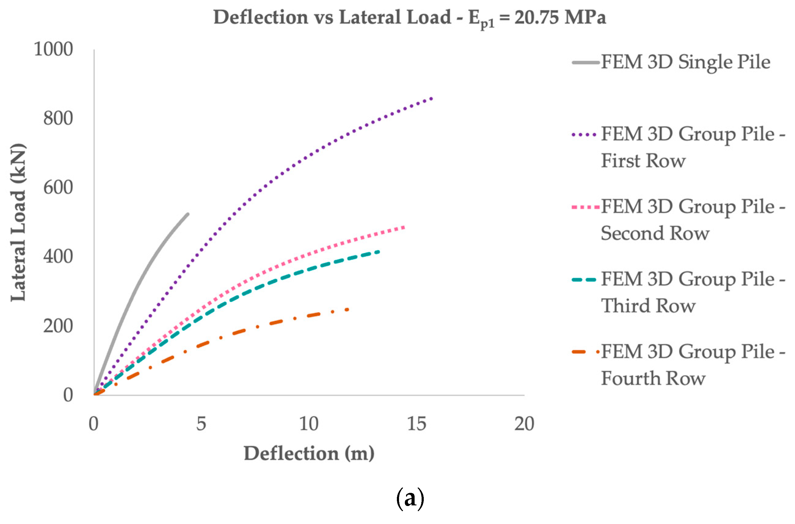
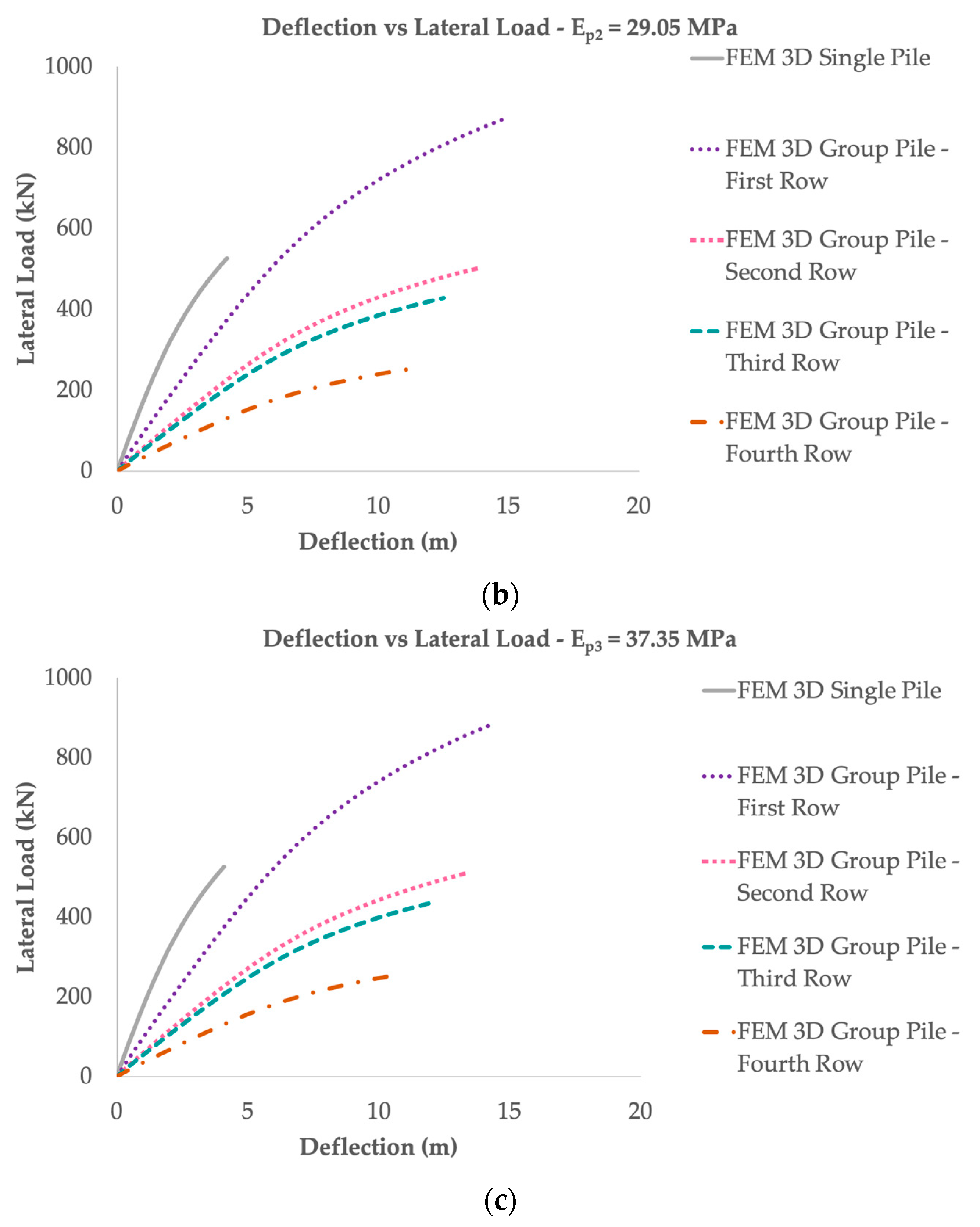
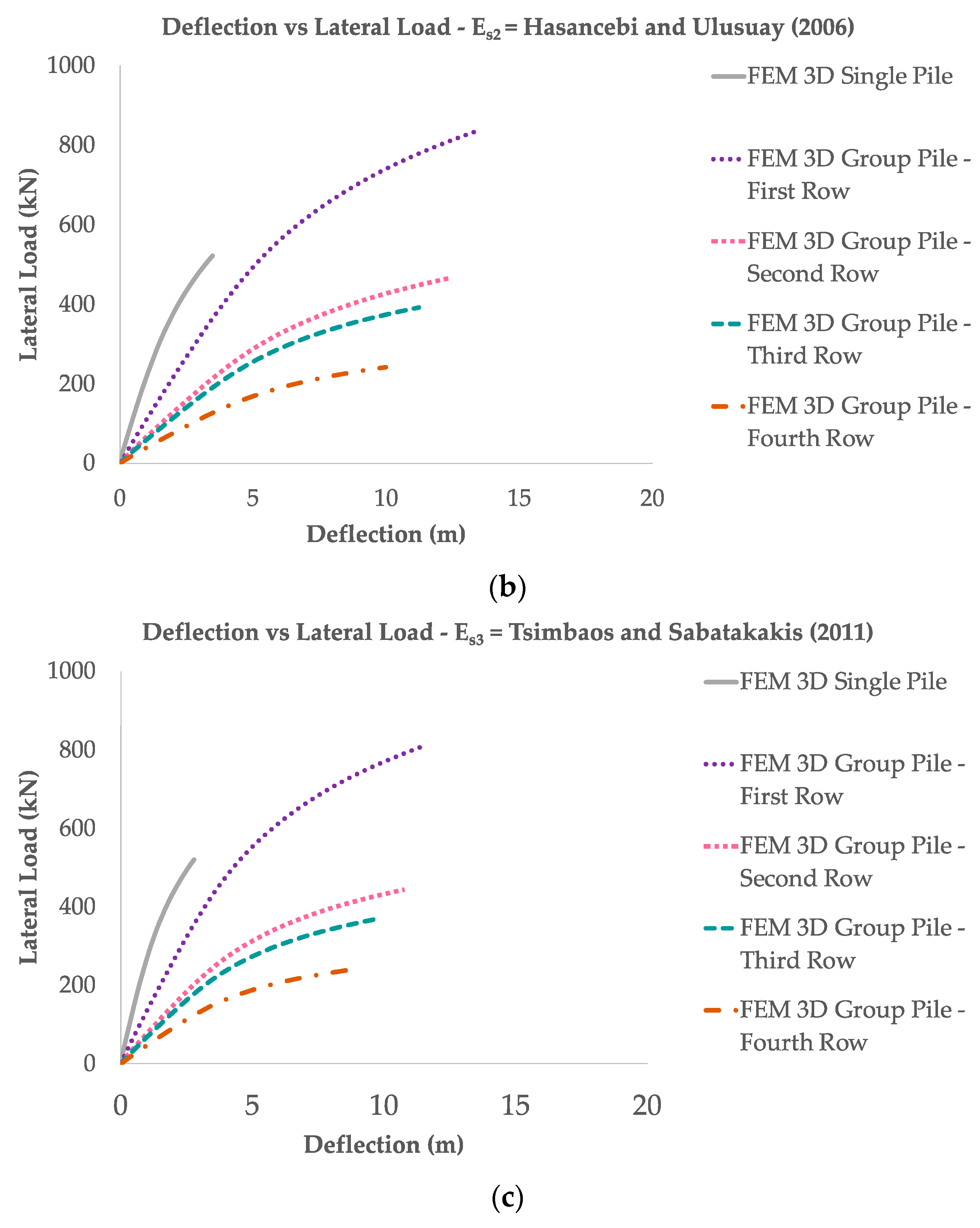
4.1. Group Pile Lateral Load Capacity

The failure mechanism occurred as usual (Figure 8). Pile bending occurs to the right (passive wedge) from a depth of 0.00–10.00 m. It is appropriate that the small diameter pile shows a wedge failure up to 5D at a shallow depth with deflection decreasing to zero at more than 8D below the soil surface [4].

Figure 9, Figure 10 and Figure 11 shows a graph of the lateral load that the pile can withstand and the value of the deflection. If the pile is given a load of 542.453 kN for condition 690.240 kN for condition 2, and 822.309 kN for condition 3, the combination lateral loads effect, pile stiffness, and soil stiffness effect on a 3D single pile analysis with a square pile cap can withstand a load of 300 kN lower than the given load under these three conditions. In the pile group analysis, if the pile is given a load of 7051.887 kN for condition 1, 8973.120 kN for condition 2, and 10,690.011 kN for condition 3, the acceptable load for the first row of piles has a value of 300 kN, which is more considerable than the three loading conditions of the single pile can withstand; the second and third row are almost the same, and the fourth-row pile is 200 kN lower than the three loading conditions of the single pile can withstand. The value of the lateral capacity above is within safe limits because the ultimate lateral bearing capacity of the pile (P_ult) happens at a load of 1000 kN.

When viewed as a single pile, it can be seen from the lateral resistance that the pile in the group pile analysis with an asymmetrical pile cap can withstand a load more considerable than the single pile on the first row of piles, and the lateral resistance on the single pile has a magnitude that is almost the same as the 3D analysis of the group pile on the second row of piles with a difference of 1–10% (

Table 5. The difference of lateral resistance with the single pile.

	Lateral Resistance (kN)					The Difference of Lateral Resistance with the Single Pile (%)
	Single Pile	1st Row	2nd Row	3rd Row	4th Row	1st Row	2nd Row	3rd Row	4th Row
Combination Lateral Loads Effect
PS1, PG1	304.663	541.442	299.494	255.588	149.534	43.731	1.697	16.108	50.918
PS2, PG2	414.567	711.253	389.264	333.519	197.712	41.713	6.103	19.550	52.309
PS3, PG3	524.270	861.389	488.142	415.128	248.422	39.137	6.891	20.818	52.616
Pile Stiffness Effect
Ep1	524.270	861.389	488.142	415.128	248.422	39.137	6.891	20.818	52.616
Ep2	525.274	875.012	500.002	427.055	252.604	39.970	4.811	18.699	51.910
Ep3	526.043	885.202	509.006	436.031	255.516	40.574	3.239	17.111	51.427
Soil Stiffness Effect
Es1	524.270	861.389	488.142	415.128	248.422	39.137	6.891	20.818	52.616
Es2	522.476	837.790	465.483	391.661	242.058	37.636	10.908	25.038	53.671
Es3	520.390	812.899	443.048	367.568	237.664	35.983	14.862	29.367	54.333

Note: P_S1, P_G1 = 542.453 kN, 7051.887 kN; P_S2, P_G2 = 690.240 kN, 8973.120 kN; P_S3, P_G3 = 822.309 kN, 10,690.011 kN. E_p1 = 20.75 MPa; E_p2 = 29.05 MPa; E_p3 = 37.35 MPa. E_s1 = Maheswari et al. [23]; E_s2 = Hasancebi and Ulusay in Hammam and Eliwa [22]; E_s3 = Tsimbaos and Sabatakakis [24].

). However, if the lateral resistance is multiplied by the total number of piles (13 piles), then the overall lateral resistance of the single pile analysis is more excellent than that of the pile group analysis.

The 3D finite element of the single pile and group pile indicates a linear relationship between pile stiffness and lateral resistance, where the increase in pile stiffness will increase the lateral resistance (Figure 10). Pile stiffness affects pile response by changing soil mobilization alongside the pile. Under the same lateral load, a rigid pile will mobilize the soil to a greater depth. A flexible pile will mobilize the soil to a shallower depth with a larger degree of mobilization [32]. In addition, the 3D method indicates that the lateral resistance will decrease as the soil stiffness rises (Figure 11).

However, both methods show the same results in the combination lateral loads (Figure 9), in which the lateral resistance will rise along with the combination lateral loads. This is following the study by Liao et al. [33] that stated the load-deflection alongside the pile would increase with the applied lateral load amplitude. Overall, observations show that the numerical model is reliable for the improvement of the soil−pile reaction while decreasing the overall flexural stiffness of the pile friction [4].

The average difference in the lateral capacity of the first to the fourth row of piles obtained by 3D group pile analysis compared with single pile analysis is 40% for the first row, 1–10% for the second row, 20% for the third row, and 50% for the fourth row (Table 5).

The front row piles have the largest resistance values, followed by the second, third, and fourth row piles. In other words, the 3D finite element model exaggerates the shadow effect behind the leading row [5]. Walsh [34] revealed that the overall lateral load is shared among each pile in the group. Each pile pushes against the soil behind it, creating a shear zone in the soil.

These shear zones begin to enlarge and overlap as the load increases and the distance between piles becomes adjacent. Overlap between two piles in the same row is called the edge effect, while overlap between piles in different rows is known as the shadow effect. All these group interactions result in reduced lateral resistance per pile. The leading row of piles has the highest resistance in the group as it only suffers from edge effects. Piles in other rows, however, have a lower resistance due to edge effects and shadow effects. The gap that forms behind the pile also reduces the resistance of the pile (Figure 12c).

Based on these observations, the location of the first row of piles that receive the most excellent lateral resistance up to the fourth row is different from the research in general conducted by some researchers [5,35]. In this case, the first to the fourth row of piles are those on the horizontal longitude, whereas in research with symmetrical pile configurations, the first row is on the vertical longitude (the farthest pile from the loading point has the greatest value, based on the theory by Walsh [34]). In that sense, the pile furthest from the loading point (piles number 5, 9, and 13) should be the first-row pile with the greatest lateral resistance, and the lateral resistance decreases until piles number 6 and 10 (Figure 12a). However, the results of this study with asymmetrical pile caps indicate that piles 1 and 2 have the greatest lateral resistance and the second-row until fourth-row piles have a lower lateral resistance (Figure 12a).

This can also be seen from the color of the deflection on the pile surface (Figure 12b), indicating that the most considerable deflection value (red color) occurs at piles 1 and 2 in the first row and decreases until the fourth row. In addition, the most considerable deflection occurs on the inclined side of the pile cap. This shows that the side slope of the pile cap can increase the shear zone and thus increase the overlap between piles and lateral resistance so that piles number 1 and 2 only experience edge effects (Figure 12c), and the greatest lateral resistance occurs in the pile opposite to the direction of loading or occurs in the horizontal longitude row of the pile. Although piles 5, 9, and 13 also experience edge-only effects, these piles are on the straight side of the pile cap so the lateral resistance is lower than piles number 1 and 2.

The load-deflection response for the group piles is more flexible than the single pile [2], as per the research results by Papadopoulou and Comodromos [35], which states that the single pile has a greater lateral resistance than the group piles under the same load. In addition, the front row of the piles has the largest deflection, and it decreases along with the number of rows. However, the results of this study are contrary to Elhakim et al. [2], which revealed that the rear row piles have a more significant deflection than the front row piles for a certain distance. This is probably due to the asymmetrical pile configuration used. Furthermore, the 3D finite element indicates that both single and group piles have a different deflection, which is 1% D for single piles and 2% D for group piles, greater than 5–10 mm and a difference of 60–70% from the single pile analysis (

Table 6. The difference of deflection with single pile.

	Deflection (mm)					The Difference of Deflection with Single Pile (%)
	Single Pile	1st Row	2nd Row	3rd Row	4th Row	1st Row	2nd Row	3rd Row	4th Row
Earthquake Combination Load Effect
PS1, PG1	2.417	7.466	7.361	7.199	6.555	67.622	67.165	66.426	63.127
PS2, PG2	3.532	11.114	10.938	10.662	9.572	68.220	67.709	66.873	63.101
PS3, PG3	4.972	16.257	15.977	15.539	13.824	69.416	68.880	68.003	64.034
Pile Stiffness Effect
Ep1	4.972	16.257	15.977	15.539	13.824	69.416	68.880	68.003	64.034
Ep2	4.808	15.367	15.101	14.690	13.090	68.712	68.161	67.270	63.270
Ep3	4.692	14.756	14.500	14.108	12.588	68.203	67.641	66.742	62.726
Soil Stiffness Effect
Es1	4.972	16.257	15.977	15.539	13.824	69.416	68.880	68.003	64.034
Es2	3.939	13.852	13.616	13.241	11.768	71.564	71.071	70.251	66.528
Es3	3.140	11.964	11.763	11.438	10.154	73.755	73.306	72.548	69.0.76

Note: P_S1, P_G1 = 542.453 kN, 7051.887 kN; P_S2, P_G2 = 690.240 kN, 8973.120 kN; P_S3, P_G3 = 822.309 kN, 10,690.011 kN. E_p1 = 20.75 MPa; E_p2 = 29.05 MPa; E_p3 = 37.35 MPa. E_s1 = Maheswari et al. [23]; E_s2 = Hasancebi and Ulusay in Hammam and Eliwa [22]; E_s3 = Tsimbaos and Sabatakakis [24].

).

When compared with the single pile analysis, the group pile with asymmetrical pile cap and pile configuration does not affect the behavior of lateral resistance and deflection, whereas the results of the 3D analysis of the group piles and single pile showed that the deflection and lateral resistance would increase along with the combination lateral loads (Figure 9). With increasing effect, the combination lateral loads increase the deflection by 1.00–5.00 mm (30%) and the lateral resistance to 80–100 kN (20%) (Table 5 and Table 6).

However, increasing pile stiffness will reduce the deflection rate and increase the lateral resistance (Figure 10). An increase in the pile stiffness effect reduces the deflection to 1.00 mm (3–5%) and increases the lateral resistance to 1–10 kN (1–2%) (Table 5 and Table 6). This is consistent with Wang et al. [4] which stated that the flexural stiffness of the pile will slightly increase the lateral resistance.

In addition, rigid pile deflection under the same lateral load will reduce pile tip displacement as E_s increases [3,4]. Soil stiffness has a negative correlation with deflection and lateral loads (Figure 11), where both factors will decrease with increasing soil stiffness. With an increase in the soil stiffness effect, the deflection decreases by 1.00–2.00 mm (15–20%) and increases the lateral resistance to 1–20 kN (1–5%) (Table 5 and Table 6). Zhou et al. [3] found the deflection did not rise significantly when E_s increased.

4.2. p-Multiplier

The p-multiplier (p_m) parameter was used to consider group pile effects. The p-multiplier is calculated using the single pile p-y curve divided by the p-y curve for each pile group row. The p-y curve obtained with the help of finite difference software for the single pile and the group pile is calculated using the API [7] method approach with ultimate soil resistance, p_u, from the first row to the fourth row also being obtained based on numerical calculations based on the finite difference method (Figure 13a). Pile modeling with the finite difference method is the same with the 3D finite element method and the relationship between soil resistance and deflection (p-y curve) was taken at a depth of 0.00 m to match the pile group’s deflection output from the 3D finite element analysis.

The 3D finite element analysis found that a higher p-multiplier was followed by a larger deflection. This is in contrast to the study by Zhu et al. [8], where p_m decreases gradually with y, revealing that the pile group effect depends on the pile deflection. As the pile deflection increases, the protective effect becomes more significant and causes a considerable decrease in p_m. This difference may occur due to the diversity of methodology, soil type, and geometric parameters used between studies to derive the p-multiplier. Other reasons that can cause this difference in results are the reduction of the earth pressure limit, group effect, and inconstant depth [36].

The biggest reason for this study is the irregular pile configuration and the greatest lateral resistance lies in the direction opposite to the loading direction. Papadopoulou and Comodromos [35] have shown that the p-multiplier depends on the configuration of the group piles. The constant value of the p-multiplier based on the analytical method despite the increasing deflection is because the p-multiplier is based on the distance between the piles and the pile diameter. Thus, the deflection does not affect the p-multiplier.

This study shows that the analytical method from FEMA P-751 [14], Reese and Impe [15], and AASHTO [16] does not show the effect function of combination lateral loads, pile stiffness, and soil stiffness. Although the p-multiplier changes with increasing pile deflection [11].

Figure 13b shows the p-multiplier value based on the numerical method and analytical method obtained by 0.79 based on FEMA P-751 [14], 0.80 based on Reese and Impe [15], and 0.93 based on AASHTO [16] for the first-row pile. In the second row, it is 0.57 from FEMA P-751 [14], 0.40 from Reese and Impe [15], and 0.58 from AASHTO [16]. In the third- and fourth-row pile, it is 0.41 from FEMA P-751 [14], 0.30 from Reese and Impe [15], and 0.58 from AASHTO [16]. The analytical method used by AASHTO [16] yielded the highest p_m values for the three variables, followed by Reese and Impe [15] and FEMA P-751 [14]. This may be because AASHTO [16] used data from most of the tests in the 3 × 3 pile group, and there were no fixed-head conditions in the AASHTO [16] database. Reese and Impe [15] generally matches or approaches the p_m value from the 3D finite element method obtained in this study. This is appropriate because Reese and Impe [15] not only considers the effects of the adjacent, parallel piles but also considers misaligned piles concerning the applied load.

In addition, the first row of piles has the largest p_m value, and its value continues to decrease as the row of piles increases. This is in accordance with the behavior of the lateral load capacity, where the farther the pile is from the lateral load, the lower the p_m will be. Zhou and Tokimatsu [11] also revealed that the p-multiplier decreases approximately from the leading row to the last row in the subgroup, whereas the p-multiplier of the leading row in the final subgroup is equal to or even greater than the last row in the front group.

This shows that the proposed method was less effective in this study. In this case, it is necessary to do further research by not only dividing the lateral resistance of the pile group by a single pile to get the p-multiplier value, but also by adding another multiplier or dividing factor to get the p-multiplier value by the existing theory.

5. Conclusions

With the increase of the earthquake intensity in Indonesia, especially in Malang, East Java, and the rarity of research experiments carried out to observe the behavior of pile groups in asymmetrical pile caps and pile configurations, it is important to conduct research in this area. This research was carried out to determine the response of the group pile; that is, the lateral resistance of the soil and p-multiplier to earthquake loads with an asymmetrical pile cap and pile configuration. The results of which were carried out using a numerical method based on the 3D finite element. Conclusions based on the above analysis can be drawn as follows:

• Lateral load capacity of group piles:
  • Asymmetrical pile caps and pile configurations do not affect the behavior of lateral resistance and deflection, only producing different lateral resistance values with a difference of 1–50% and 60–70% for deflection values compared to the finite element 3D single pile analysis. On the effect of combination lateral loads, pile stiffness, and soil stiffness, the analysis of lateral resistance and deflection of group piles with 3D finite elements is in good agreement with single pile 3D finite elements.
  • In addition, the asymmetrical shape of the pile cap and pile configuration affects the location of the greatest lateral resistance. The slope of the pile cap can increase the shear zone, thus increasing the lateral resistance so that the most remarkable overlap occurs in the direction opposite to the loading direction.
• p-multiplier:
  • In this study, the proposed method is less effective with asymmetrical pile configurations, where the value of the p-multiplier increases with an increasing deflection. In future research, it is necessary to not solely divide the lateral resistance of the pile group by a single pile to get the p-multiplier value. In this case, further studies are required to be carried out with the possibility of adding another multiplying or dividing factor.
  • Results from Reese and Impe [15] generally match or approach the p_m value from the 3D finite element method obtained in this study. This is appropriate because Reese and Impe [15] not only considers the effects of adjacent, parallel piles, but also considers misaligned piles concerning the applied load. The 3D finite element method was within the range suggested by the design recommendations.

References

1. National Earthquake Study Library Team. Peta Sumber dan Bahaya Gempa Indonesia Tahun 2017 [Map of Indonesia Earthquake Sources and Hazards in 2017]; Pusat Penelitian dan Pengembangan Perumahan dan Permukiman Badan Penelitian dan Pengembangan Kementrian Pekerjaan Umum dan Perumahan Rakyat: Jakarta, Indonesia, 2017. [Google Scholar]
2. Elhakim, A.F.; El Khouly, M.A.A.; Awad, R. Three Dimensional Modeling of Laterally Loaded Pile Groups Resting in Sand. HBRC J. 2016, 12, 78–87. [Google Scholar] [CrossRef]
3. Zhou, P.; Zhou, H.; Liu, H.; Li, X.; Ding, X.; Wang, Z. Analysis of lateral response of Existing Single Pile Caused by Penetration of Adjacent Pile in Undrained Clay. Com. Geotech. 2020, 126, 103736. [Google Scholar] [CrossRef]
4. Wang, H.; Wang, L.Z.; Hong, Y.; He, B.; Zhu, R.H. Quantifying the Influence of Pile Diameter on the Load Transfer Curves of Laterally Loaded Monopile in Sand. App. Ocean. Res. 2020, 101, 102196. [Google Scholar] [CrossRef]
5. Lin, Y.; Lin, C. Scour Effects on Lateral Behavior of Pile Groups in Sands. Ocean. Eng. 2020, 208, 107420. [Google Scholar] [CrossRef]
6. Cao, G.; Ding, X.; Yin, Z.; Zhou, H.; Zhou, P. A New Soil Reaction Model for Large-Diameter Monopiles in Clay. Comput. Geotech. 2021, 137, 104311. [Google Scholar] [CrossRef]
7. API. Petroleum and Natural Gas. Industries-Specific Requirements for Offshore Structures: Part 4-Geotechnical and Foundation Design Considerations ISO 19901–4:2003; American Petroleum Institute: Washington, DC, USA, 2014. [Google Scholar]
8. Zhu, B.; Wen, K.; Kong, D.; Zhu, Z.; Wang, L. A Numerical Study on the Lateral Loading Behaviour of Offshore Tetrapod Piled Jacket Foundations in Clay. App. Ocean. Res. 2018, 75, 165–177. [Google Scholar] [CrossRef]
9. Jia, J. Soil Dynamics and Foundation Modeling: Offshore and Earthquake Engineering; Springer: Bergen, Norway, 2018. [Google Scholar]
10. Das, B.M. Principles of Foundation Engineering, 7th ed.; Thomson: Toronto, ON, Canada, 2011. [Google Scholar]
11. Badan Standardisasi Nasional. Perencanaan Ketahanan Gempa Untuk Gedung dan Non Gedung [SNI 1726:2019] Earthquake Resistance Planning for Buildings and Non-Buildings [SNI 1726:2019]; Badan Standardisasi Nasional: Jakarta, Indonesia, 2019. [Google Scholar]
12. Zhou, Y.; Tokimatsu, K. Numerical Evaluation of Pile Group Effect of a Composite Group. Soils Found. 2018, 58, 1059–1067. [Google Scholar] [CrossRef]
13. Brown, D.A.; Morrison, C.; Reese, L.C. Lateral Load Behavior of Pile Group in Sand. J. Geotech. Eng. Am. Soc. Civil. Eng. 1988, 114, 1261–1276. [Google Scholar] [CrossRef]
14. FEMA P-751. NEHRP Recommended Seismic Provisions: Design Examples; National Institute of Building Sciences: Washington, DC, USA, 2009. [Google Scholar]
15. Reese, L.C.; Impe, W.F.V. Single Piles and Pile Groups Under Lateral Loading, 2nd ed.; CRC Press: Boca Raton, FL, USA, 2011. [Google Scholar]
16. American Association of State Highway and Transportation Officials (AASHTO). AASHTO LRFD 2012 Bridge, Design Specifiations, Customary U.S. Units; American Association of State Highway and Transportation Officials: Washington, DC, USA, 2012. [Google Scholar]
17. Kumar, K. Basic Geotechnical Earthquake Engineering; New Age International Publisher: New Delhi, India, 2008. [Google Scholar]
18. Poulos, H.G. Tall Building Foundation Design; Taylor & Francis Group: Abingdon, UK, 2017. [Google Scholar]
19. Akin, M.K.; Kramer, S.L.; Topal, T. Empirical Correlations of Shear Wave Velocity (Vs) and Penetration Resistance (SPT-N) for Different Soils in an Earthquake-Prone Area (Erbaa-Turkey). Eng. Geo. 2011, 119, 1–17. [Google Scholar] [CrossRef]
20. Fabbrocino, S.; Lanzano, G.; Forte, G.; de Magistris, F.S.; Fabbrocino, G. SPT Blow Count vs. Shear Wave Velocity Relationship in the Structurally Complex Formations of the Molise Region (Italy). Eng. Geo. 2015, 187, 84–97. [Google Scholar] [CrossRef]
21. Rahimi, S.; Wood, C.M.; Wotherspoon, L.M. Influence of Soil Aging on SPT-Vs Correlation and Seismic Site Classification. Eng. Geo. 2020, 272, 105653. [Google Scholar] [CrossRef]
22. Hammam, A.H.; Eliwa, M. Comparison between Results of Dynamic & Static Moduli of Soil Determined by Different Methods. HBRC J. 2013, 9, 144–149. [Google Scholar]
23. Maheswari, R.U.; Boominathan, A.; Dodagoudar, G.R. Use of Surface Waves in Statistical Correlations of Shear Wave Velocity and Penetration Resistance of Chennai Soils. Geotech. Geo. Eng. 2010, 28, 119–137. [Google Scholar] [CrossRef]
24. Tsimbaos, G.; Sabatakakis, N. Empirical Estimation of Shear Wave Velocity from in Situ Tests on Soil Formations in Greece. Bull. Eng. Geo. Env. 2011, 70, 291–297. [Google Scholar] [CrossRef]
25. Comodromos, E.M.; Papadopoulou, M.C. Explicit Extension of the p–y Method to Pile Groups in Cohesive Soils. Com. Geotech. 2013, 47, 28–41. [Google Scholar] [CrossRef]
26. Raikar, P. Modelling Soil Damping for Suction Pile Foundations. Master’s Thesis, Delft University of Technology, Delft, The Netherlands, 2016. [Google Scholar]
27. Poulos, H.G.; Davis, E.H. Pile Foundation Analysis and Design; Wiley: New York, USA, 1980; Available online: https://trid.trb.org/view/164430 (accessed on 24 May 2022).
28. Li, Z.; Kotronis, P.; Escoffier, S. Numerical Study of the 3D Failure Envelope of a Single Pile in Sand. Com. Geotech. 2014, 62, 11–26. [Google Scholar] [CrossRef]
29. Bentley Communities. Manuals-PLAXIS: Plaxis 3D Material Models. Available online: https://communities.bentley.com/products/geotech-analysis/w/plaxis-soilvision-wiki/46137/manuals---plaxis (accessed on 25 May 2022).
30. Tjie-Liong, G. Common Mistakes on the Application of Plaxis 2D in Analyzing Excavation Problems. Int. J. App. Eng. Res. 2014, 9, 8291–8311. [Google Scholar]
31. Ilori, A.O.; Udoh, N.E.; Umenge, J.I. Determination of soil shear properties on a soil to concrete interface using a direct shear box apparatus. Int. J. Geo. Eng. 2017, 8, 1–14. [Google Scholar] [CrossRef]
32. Zhang, Y.; Andersen, K.H.; Tedesco, G. Ultimate Bearing Capacity of Laterally Loaded Piles in Clay—Some Practical Considerations. Mar. Struct. 2016, 50, 260–275. [Google Scholar] [CrossRef]
33. Liao, W.; Zhang, J.; Wu, J.; Yan, K. Response of Flexible Monopile in Marine Clay under Cyclic Lateral Load. Ocean. Eng. 2018, 147, 89–106. [Google Scholar] [CrossRef]
34. Walsh, J. Full-Scale Lateral Load Test of a 3x5 Pile Group in Sand. Master’s Thesis, Brigham Young University, Provo, UT, USA, 2005. [Google Scholar]
35. Papadopoulou, M.C.; Comodromos, E.M. On the Response Prediction of Horizontally Loaded Fixed-Head Pile Groups in Sands. Com. Geo. 2010, 37, 930–941. [Google Scholar] [CrossRef]
36. Georgiadis, K.; Sloan, S.W.; Lyamin, A.V. Undrained Limiting Lateral Soil Pressure on a Row of Piles. Com. Geotech. 2013, 54, 175–184. [Google Scholar] [CrossRef]
Figure 1. Lateral earth pressure semi-basement wall.
Applsci 12 08142 g001
Figure 2. Comparison of the p-y curves of single and group piles.
Applsci 12 08142 g002
Figure 3. Study location.
Applsci 12 08142 g003
Figure 4. Soil investigation location.
Applsci 12 08142 g004
Figure 5. Bored pile elevation and N-SPT data.
Applsci 12 08142 g005
Figure 6. Finite element group pile modeling (a) group pile, (b) single pile.
Applsci 12 08142 g006
Figure 7. Indonesian Earthquake Zone Map (a) amplification factor for a short period (Ss), (b) amplification factor for 1.0 s period (S1).
Applsci 12 08142 g007
Figure 8. Failure mechanism of the group pile.
Applsci 12 08142 g008
Figure 9. Lateral load capacity vs. deflection (a) PS1, PG1, (b) PS2, PG2, (c) PS3, PG3.
Applsci 12 08142 g009aApplsci 12 08142 g009b
Figure 10. Lateral load capacity vs. deflection (a) Ep1 = 20.75 MPa, (b) Ep2 = 29.05 MPa, (c) Ep3 = 37.35 MPa.
Applsci 12 08142 g010aApplsci 12 08142 g010b
Figure 11. Lateral load capacity vs. deflection (a) Es1 = Maheswari et al. [23], (b) Es2 = Hasancebi and Ulusay in Hammam and Eliwa [22], (c) Es3 = Tsimbaos and Sabatakakis [24].
Applsci 12 08142 g011aApplsci 12 08142 g011b
Figure 12. Pile configuration, (a) pile configuration, (b) deflection surface, (c) overlapping of failure zones.
Applsci 12 08142 g012
Figure 13. (a) p-y curve (b) p-multiplier.
Applsci 12 08142 g013