1. Introduction
Recent years have witnessed tremendous development of 3D capture devices and reconstruction technologies, and point clouds have become a crucial data structure for storage and transmission of 3D data. A point cloud is an unordered set of points in 3D space, usually represented by their coordinates, corresponding to the geometry, and each point may have its associated attributes, such as color and reflectance. Through these properties it can practically represent arbitrary 3D objects or scenes. As more and more point cloud content is made available and non-compressed point cloud requires a huge volume of data, the development of appropriate coding solutions becomes essential.
Motivated by the huge success of deep neural networks (DNN)-based image and video compression [
1,
2,
3,
4], several studies have been devoted to the use of deep learning for PCAC. Generally, they follow the VAE framework of image compression but in different point cloud representations to perform the attribute compression, such as the point-based PointNet series [
5,
6] architecture in [
7] (Deep-PCAC), voxel-based 3D dense convolutions in [
8] and sparse convolution in [
9] (SparsePCAC). Specially, Quach et al. [
10] builds a mapping between 3D point clouds and 2D grids, and utilizes the existing image compression method to encode and decode the 2D grids. However, the performance of these learning-based solutions still lags behind that of traditional G-PCC. How to develop the potential of learning-based approaches to outperform the traditional methods is still a challenging task.
Point cloud compression can be divided into two main categories: geometry compression and attribute compression. Geometry compression involves compression of point coordinates in 3D space while attribute compression involves compression of point attributes. In this paper, we focus on point cloud attribute compression and assume the geometry information is known. Without loss of generality, we assume that the attributes are colors represented as (R, G, B) triplets in RGB color space. Considering the efficiency of sparse convolution processing sparsely distributed point clouds, we establish a PCAC framework on top of the sparse convolution [
11] based VAE structure. It should be noted that, in the proposed framework, we overcome the defect of other learning-based methods in capturing the long range dependencies in the use of stacked convolution operations. The non-local attention mechanism module (NLAM) is introduced into the proposed VAE structure to capture both local and global correlations among voxels. The non-local attention masks are applied at different layers to distinguish the importance of latent features in both positions and channels dimensions for better compression. Furthermore, in the existing learning-based PCAC methods, the network parameters are learned by jointly minimizing bitrate and distortion at a particular trade-off. To this end each trade-off needs an independent model. Multiple independent models require large memory to store and transmission, which puts great limitations on the practical applications. Inspired by the variable bitrate compression methods of image compression [
12,
13,
14], we propose a modulation network to adaptively modify the latent features of different layers. This modulation network is based on parameter sharing multilayer perceptron (MLP) and the modification is implemented by simple yet effective channel-wise production. Experimental results have shown that the proposed lightweight but effective modulation network successfully achieve variable bit compression in a single network with only acceptable performance loss.
We evaluate the performance on voxelized 8i Voxelized Full Bodies (8iVFB) [
15] which has been adopted by MPEG as the standard test set and experiments are executed under common test conditions. Our proposed method achieves the state-of-the-art coding performance compared with other existing learning-based methods learning-based methods and further reduces the performance gap with the latest MPEG G-PCC coding software TMC13 version 14 (TMC13v14). Specifically, for the Bjøntegaard Delta rate (BD-rate), the proposed method outperforms Deep-PCAC and SparsePCAC by 50.7% reduction and 6.3% reduction, respectively, and reduces the gap with TMC13v14 to 29.3%.
The primary contributions of this paper include:
(1) This paper explores the application of attention mechanism in point cloud attribute compression. The attention mechanism is integrated in which a non-local attention module is developed to capture the local and global correlations in both spatial and channel dimensions, which is demonstrated to improve the performance of current VAE coding framework.
(2) For practical applications, the proposed modulation network adaptively modifies the latent features of different sparse convolutional layers in a single network, which avoids memory cost of storing multiple networks for multiple bitrates.
(3) We establish an end-to-end learning-based PCAC framework which achieves the state-of-the-art compression performance compared to other existing learning-based methods and further reduces the gap with the latest MPEG-PCC reference software TMC13 version 14.
The remainder of this paper is organized as follows.
Section 2 gives a brief review of related works.
Section 3 describes the framework of our proposed point cloud attribute autoencoder, the non-local attention module, and the variable rate autoencoder network.
Section 4 first depicts the training and testing details. Then, this section presents objective quality comparison results, subjective quality comparison results, and ablation studies. Finally, concluding remarks and future works are described in
Section 5.
3. Point Cloud Attribute Variational Autoencoder
Due to the good exploration of sparse convolution on the sparsity of point cloud, we use it as the basic layer of the proposed neural network. It only computes outputs on predefined voxels and saves them into a compact sparse tensor. The sparse tensor is represented by a set of coordinates
of these voxels and corresponding features
which can be written in a simple form:
where
N is the number of point/feature, and
C is the number of channel. Then, sparse convolution can be defined as follows:
where
and
are input and output coordinates, respectively.
and
are input and output feature vectors at coordinate
u (i.e.,
), respectively.
defines a 3D convolutional kernel centered at
u with offset
i in
.
is kernel weights.
In 3D dense convolution, the convolution is implemented on each voxel in the 3D dense grid. If the centered voxel is empty and its 3D kernel covers any occupied voxel, the centered voxel will be filled by the value generated by the convolution, which leads to the occupied voxels gradually increase. In contrast, the sparse convolution works strictly on submanifolds of data, hence the generated values also only exist on the submanifolds. Therefore, after deep convolution layers, the point cloud structure could still remain the sparsity, avoiding the difficulty of compression caused by feature map dilation.
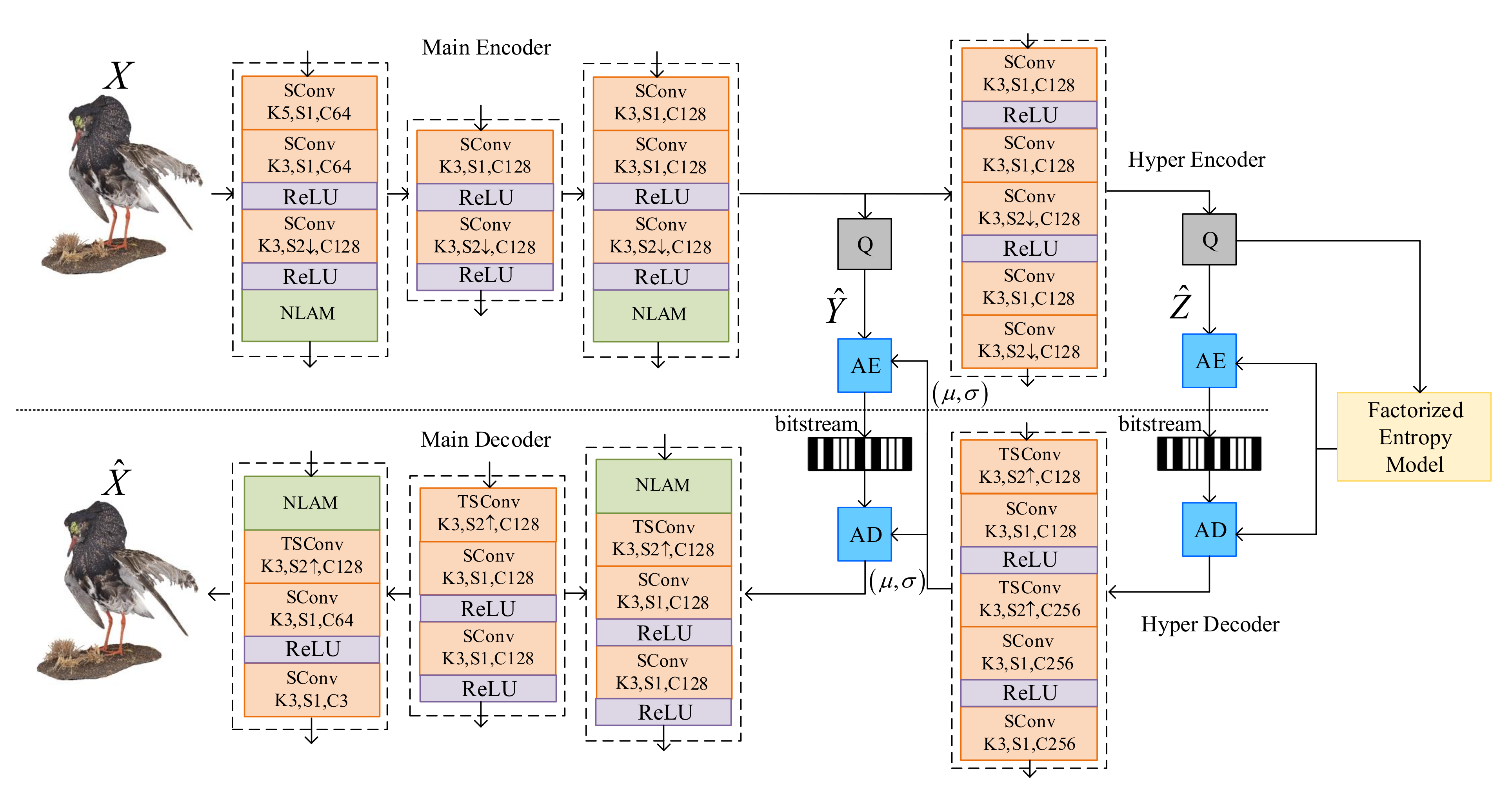
3.1. General Framework
Figure 1 illustrates the detailed proposed VAE architecture. It is established on a VAE structure [
23], with non-local attention modules in main encoder-decoder pairs. As the geometric information has been assumed decoded, the coordinates
and
in Equation (
2) have been already known in encoder and decoder.
X and
denote the feature part of the sparse tensor, which are the input attribute and the reconstructed output color attribute of the point cloud, respectively.
Main encoder with quantization
Q is used to generate quantized latent features
and main decoder decodes the features into the reconstructed point cloud. The main encoder consists of Sparse Convolutional (SConv) layers, followed Rectified Linear Unit (ReLU) activation layers and NLAMs. Note that the first convolutional layer has a kernel size of 5 × 5 × 5 to cover more occupied voxels and the left SConv layers have the kernel size of 3 × 3 × 3 for deep features aggregation. The first NLAM is placed at a relatively shallow layer to capture the correlations in lower-level feature map and the second NLAM is placed at the bottleneck layer to intelligently allocate more bits in more informative areas. The structure of the main decoder is the mirror inverse of that of the main encoder. The hyper encoder generates much smaller side information as hyperpriors
.
are then processed through the hyper decoder to generate the mean and location parameters
of assumed conditional Laplacian distribution of
. Quantization and entropy coding are used to connect the encoder and decoder. The uniform noise approximation [
1] and rounding are used in the training and testing phases, respectively. Entropy coding and decoding are used to compress and decompress the quantized hyperpriors and quantized latent features, respectively.
Ideally, we want to use as few bits as possible to represent
and
while minimizing the distortion measurement between
X and
. More specifically, we wish to learn appropriate parameters of main encoder and decoder, and conditional entropy coding for better compression efficiency by minimizing the Lagrangian cost
. Distortion
between
X and
is measured by the expectation of mean squared error (MSE) in this study.
is the factor that determines the rate-distortion trade-off. Bitrate
and
is estimated using the expected entropy of latent and hyperprior features. A fully factorized density model [
1] is used to model the bit rate of
,
where the vectors
represent the parameters of each univariate distribution
(all these parameters are collectively denoted as
) and
means uniform distribution ranging from
to
. Conditioned on
, a conditional Laplacian distribution is used to estimate the probability density function (p.d.f.) of
,
where the estimated mean and location parameters
of each element
are derived from
. Finally, the bit rates of
and
are estimated using
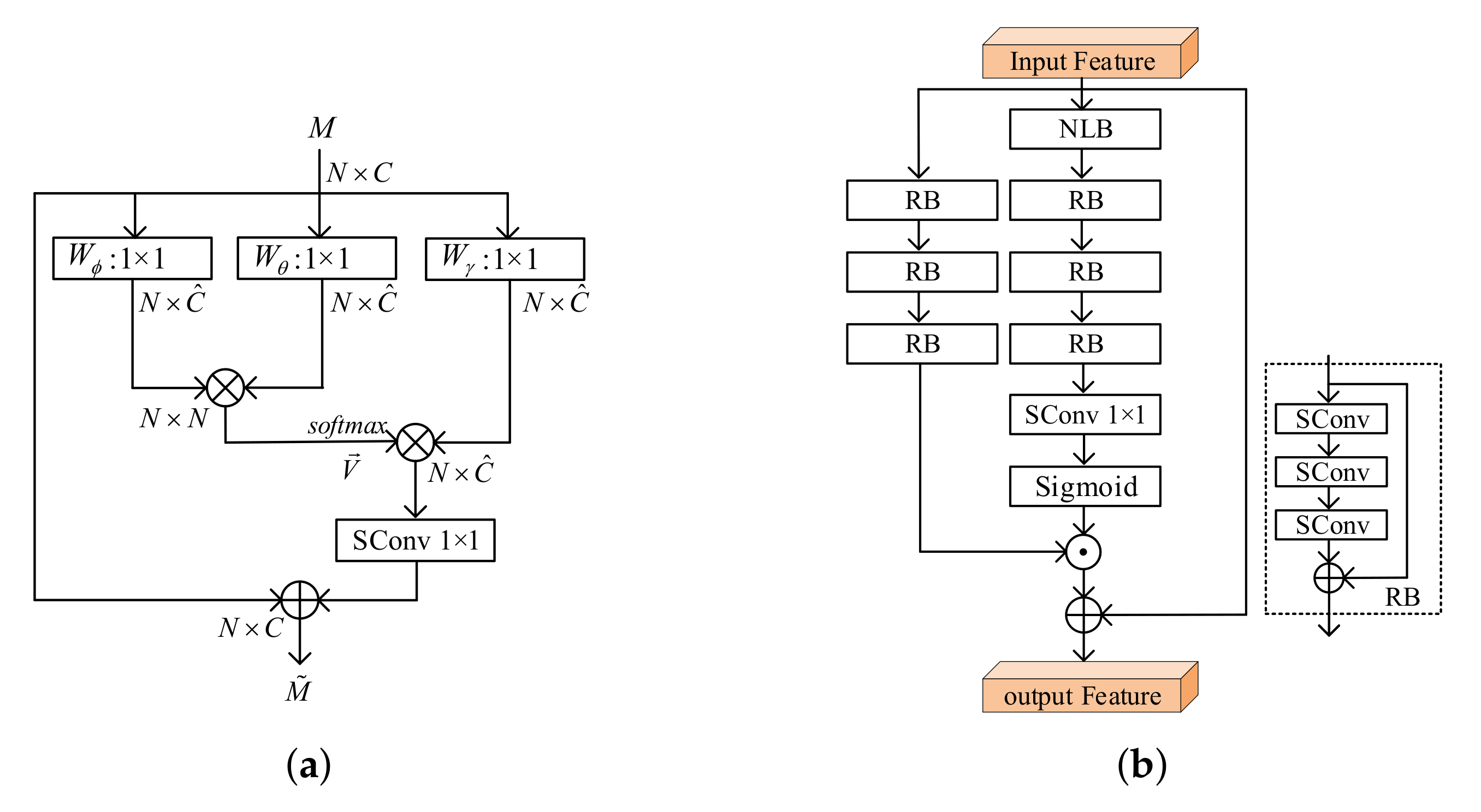
3.2. Non-Local Attention Module
The implementation of typical non-local block (NLB) [
20] in point cloud is shown in
Figure 2a. An input feature map
is output from the previous layer, where
N and
C indicate the point number and channel number. Three
convolution
,
and
are used to transform
X to different features
,
and
as
where
is the channel number of the new embeddings. Then, the similarity matrix
is calculated by a matrix multiplication as
Afterward, the softmax normalization is applied to
V to get a similarity matrix as
The output of the attention layer is obtained by matrix multiplication as
where
. By referring to the design of the non-local block, the final output is given by
where
, also implemented by a 1 × 1 convolution, acts as a weighting parameter to adjust the importance of the non-local operation with respect to the original input
M and moreover, recovers the channel dimension from
to
C. Considering global information, the non-local block effectively and adaptively diverts attention to the most important regions of an image in spatial dimension.
Inspired by the successful applications in computer vision of channel and spatial attention mechanism [
24,
25,
26,
27], we use the NLAM to generate feature maps in both dimensions. As detailed in
Figure 2b, the NLAM unit includes the main branch, mask branch and connection branch. The main branch still processes features, and can be implemented by any state-of-the-art structure such as a residual or inception block. In this work, we stack three sparse convolutional residual blocks. The mask branch focuses on non-local operation to learn a mask of the same size that weights output features from the main branch, which includes the non-local block, followed three residual blocks (RBs), one
convolution (Conv
1×1) and non-linear sigmoid activation. The sigmoid layer normalizes the output to [0, 1] and then the overall attention mask
can be written as
The third skip connection is used for faster convergence [
28]. Then the final output of NLAM can be represented as
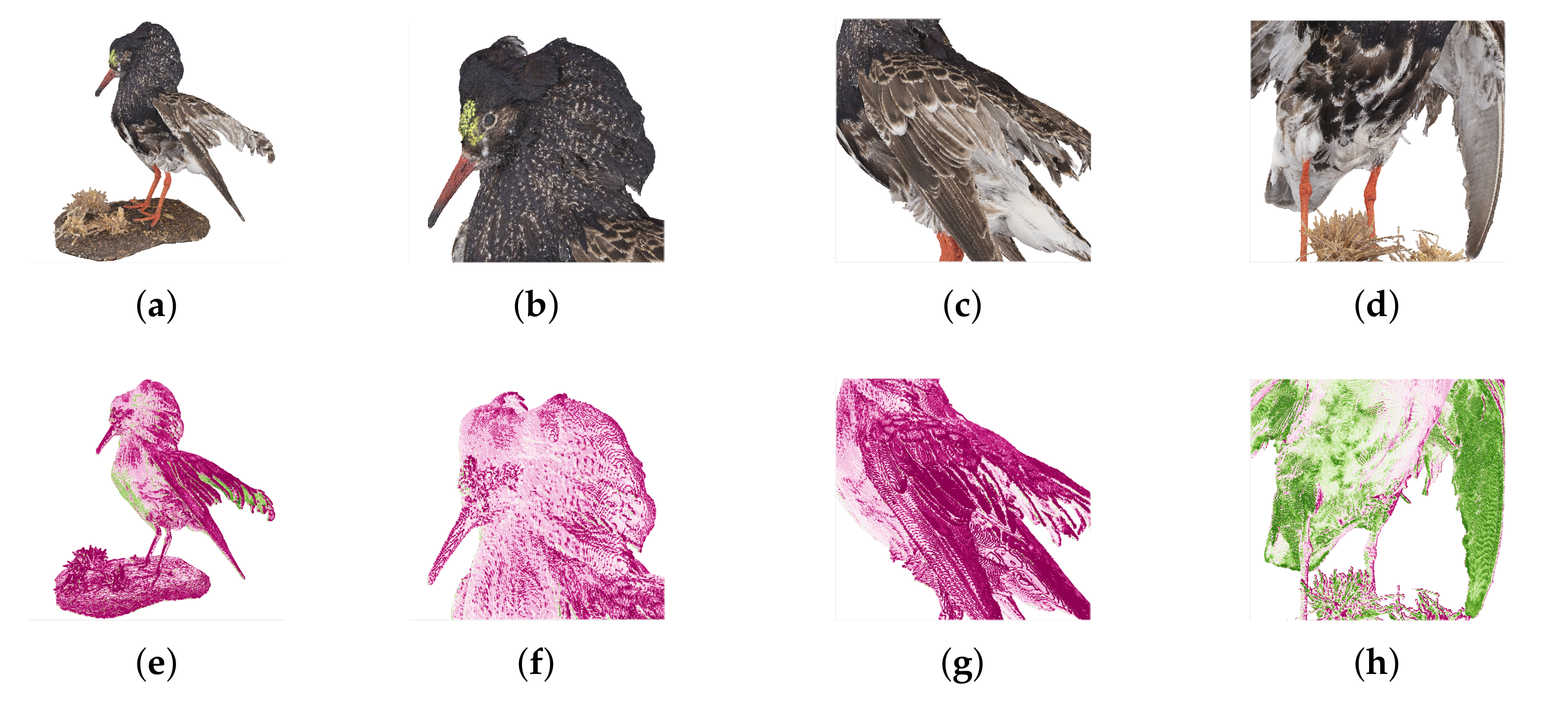
where ⨀ means element-wise product. The NLAM can provide fine-grained masks to distinguish the importance of latent features that will be further down sampled or compressed.
Figure 3 visualizes the input point cloud
Bird and its corresponding mask generated by the first NLAM. As shown in
Figure 3e–h, the closer the color is to purplish red, the closer the weight is to 1, and the closer the color is to green, the closer the weight is to 0. The textured areas such as head and upper surface of the wing are allocated higher weights to retain the original features as shown in
Figure 3b,c,f,g. The relatively plain areas such as belly and under surface of the wing are allocated lower weights to weaken their influence as shown in
Figure 3d,h.
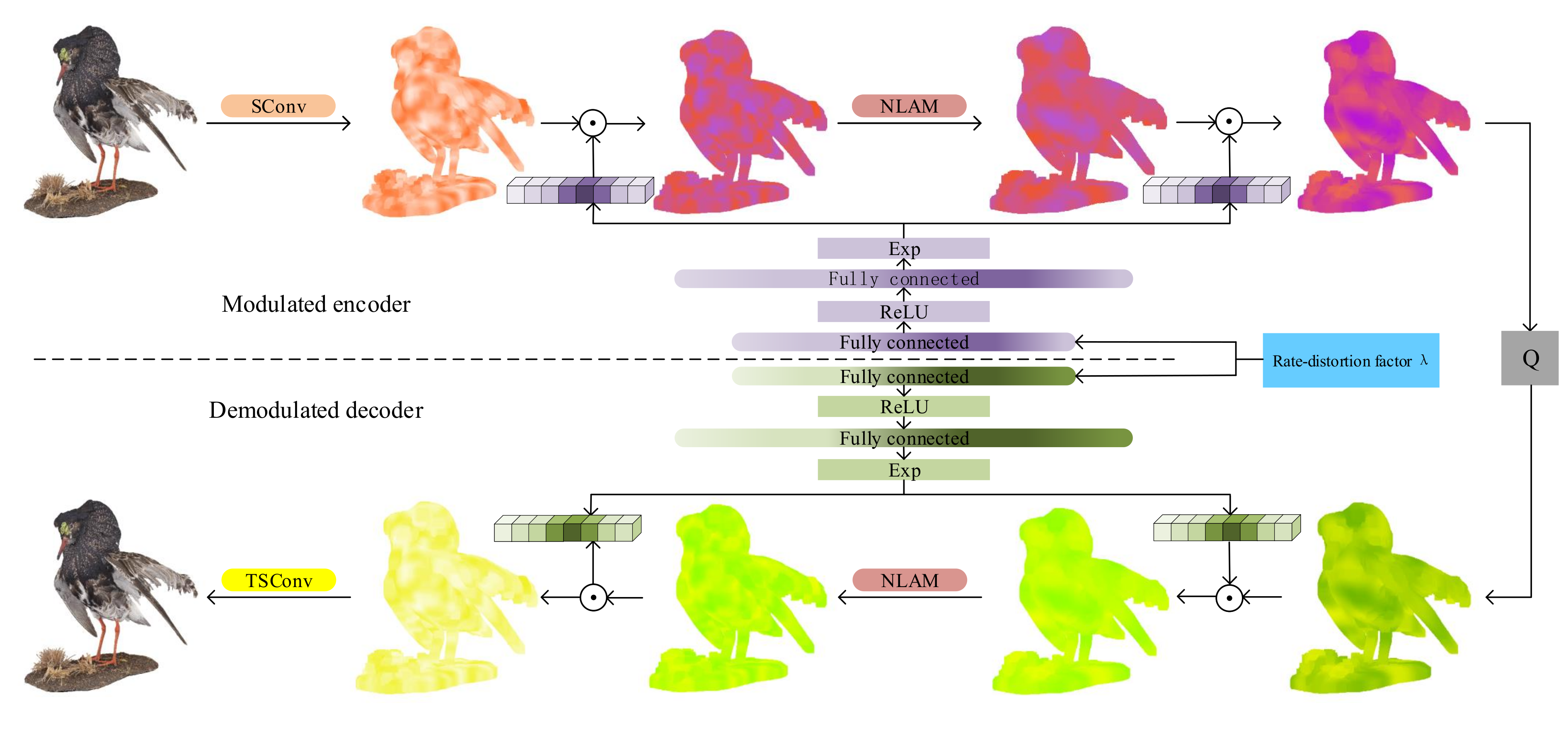
3.3. Variable Rate Autoencoder Network
Variable rate is achieved by modulating the latent features of different layers in the encoder and the decoder, which means multiplying the feature map and the modulating/demodulating vector in a channel-wise production manner.
Figure 4 shows the form of two-layer modulation, and in practice, the output of each convolution layer or attention module is modulated. Given a feature map
of channel
i in the encoder, and the output map
can be calculated as:
where
is the
i-th element of the modulating vector
.
depend on Lagrange multiplier
by
where
and
are weights matrices of two fully-connected layers. ReLU and exp are nonlinear activation and element-wise exponential function. The exponential nonlinearity guarantees positive outputs. The modulated feature maps in the decoder involve a similar calculation.
Let the SConv layers and NLAMs collectively have learnable parameters
, and modulating network has learnable parameters
, and the decoding part has parameters
and
. As a result, the overall loss function becomes
where
is a pre-defined finite set of
.
is the estimated bitrate of latent features and
is the distortion between input point cloud attribute and reconstructed point cloud attribute.
Although, for features of different layers, the parameters of the modulating network are shared, this mechanism allows multi-level and different modulation in case of more complicated networks in the future. In general, this architecture achieves effective joint training of both autoencoder and modulating network, therefore avoiding training and deploying multiple networks.
4. Experimental Results
This section describes the details of the experiments, including the train dataset, the test dataset, the anchors, and the hyper parameters for the model training. Moreover, objective quality and subjective quality comparison experiments have been performed that demonstrate the superiority of the proposed method.
4.1. Training Dataset
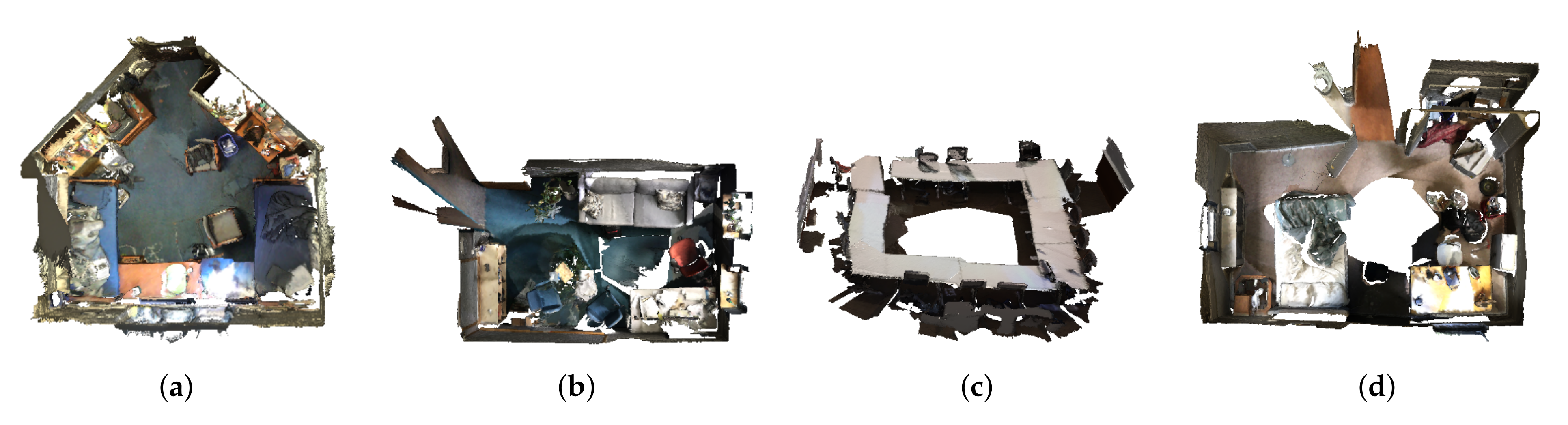
The publicly available ScanNet [
29] is a large-scale dataset with dense point cloud surface reconstructions from the indoor scenario. It consists of 1513 scans and each scan contains tens of thousands to hundreds of thousands of colored points. In our experiment, each point cloud is quantified to 1 cm.
Figure 5 shows some examples of the training dataset.
4.2. Training Details
We set
to 0.01, 0.02, 0.05, 0.09 and 0.14 to obtain the model with different bitrates. The model is trained on the dataset for 100 epochs, with the learning rate decreased from 2 × 10
to 1 × 10
. The batch size is set to 8 and the optimizer is Adam [
30] with parameter
and parameter
set to
and
, respectively. The GPU device is Nvidia GeForce RTX 3090.
4.3. Rate-Distortion Efficiency
In a lossy compression problem, one must trade off two competing costs: the bitrate of compressed representation and the distortion between the reconstructed data and input data, which is also known as rate-distortion trade-off. Following the convention, we evaluate the proposed method by comparing the rate-distortion performance with different methods, including traditional and learning-based methods.
4.3.1. Test Dataset and Anchors
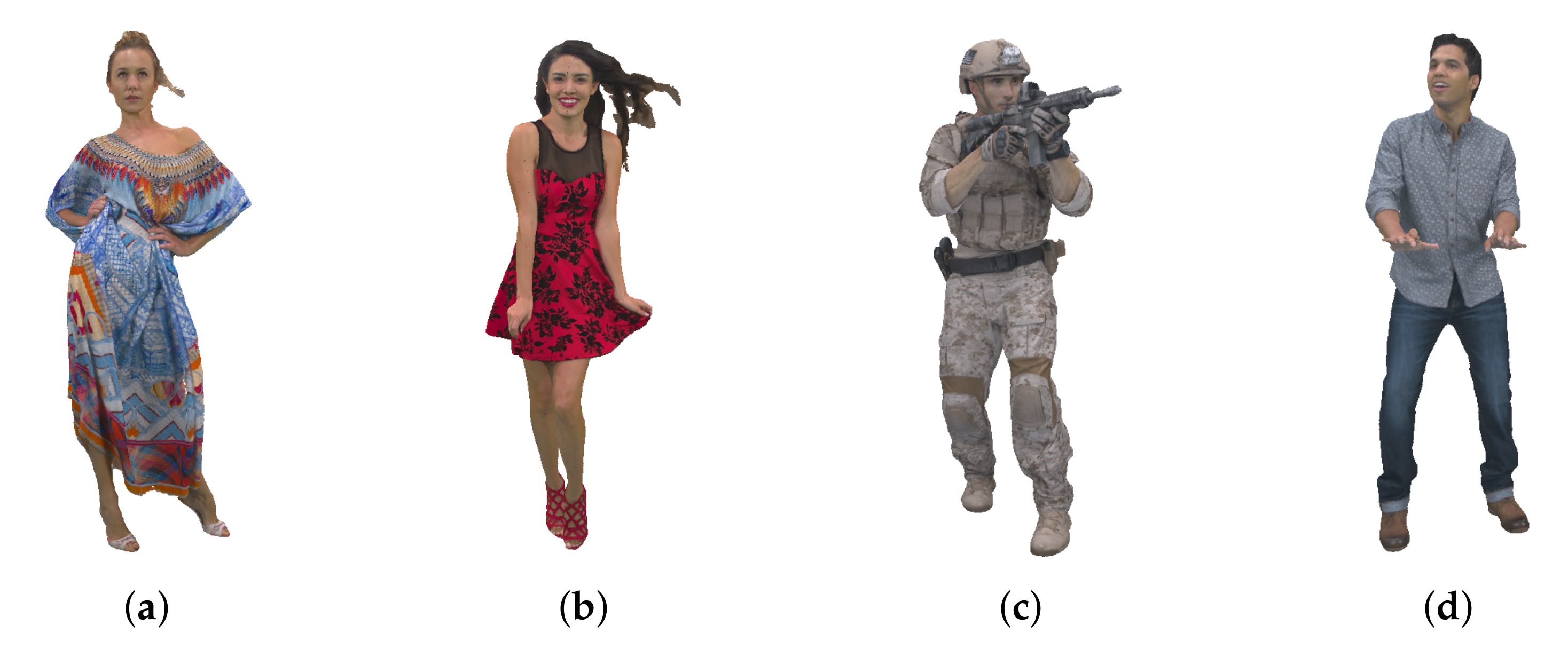
To demonstrate the performance of the proposed method, 8i Voxelized Full Bodies [
15] are selected as test dataset. As shown in
Figure 6, the geometry and attribute characteristics are completely different from the training dataset, which demonstrates the model generalization. We compare with two learning-based methods Deep-PCAC and SparsePCAC, and two different G-PCC versions: TMC13v6 and the latest and state-of-the-art TMC13v14.
4.3.2. Objective Quality Comparison
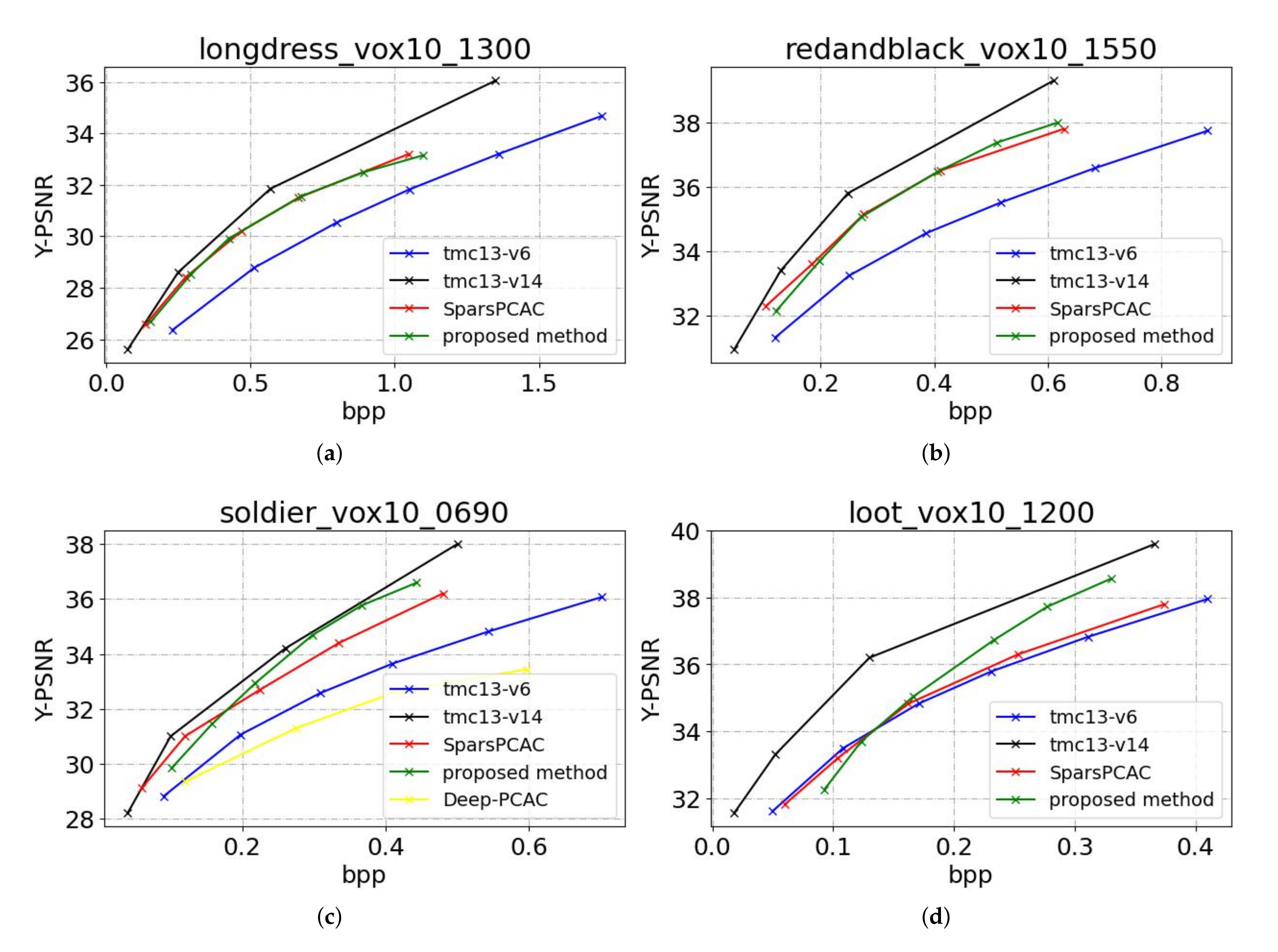
We follow the common practice to measure the bit rates (i.e., bits per points, bpp) and distortion in terms of Peak Signal-to-Noise Ratio (PSNR) in dB of the Y channel, which are computed using MPEG PCC pc error tools. As the bit rates generated by various algorithms are different, the BD-Rate (in percentage) is used to measure the overall R-D performance.
Figure 7 shows the R-D curves, and
Table 1 shows BD-rate gains. The proposed method outperforms TMC13v6 by a large margin, having 31.5% BD-rate reduction. However, the proposed method still has performance losses compared with the state-of-the-art algorithms TMC13v14. The results show that our scheme has 29.3% performance gap. For learning-based method SparsePCAC, the proposed method achieves 6.3% BD-rate reduction. For Deep-PCAC, the test sample “soldier” is used for comparison since the other three point clouds are used for training by Deep-PCAC. The proposed method achieves 50.7% BD-rate reduction.
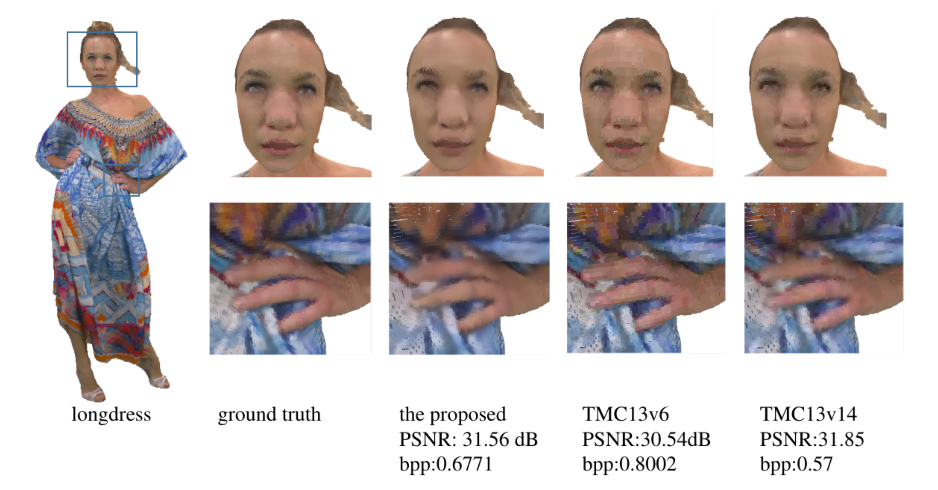
4.3.3. Subjective Quality Comparison
To show the benefits of the proposed framework in terms of subjective quality, we visualize the reconstructed point clouds of color attributes generated by different PCAC methods in
Figure 8. For a fair comparison, we obtained the visual results of all methods at approximately equal bit rates. We can see that there are apparent blurry artifacts and blocky artifacts around the longdress’s eyes and londress’s fingers for TMC13v6 and TMC13v14. In general, our method achieves the best subjective quality by having smooth texture on flat regions and retaining more clear edges in sharp regions.
4.4. Ablation Studies
In this section, we present some ablation studies to further analyze the proposed framework in the following aspects to better understand the capability of our system in practice.
4.4.1. Influence of NLAM
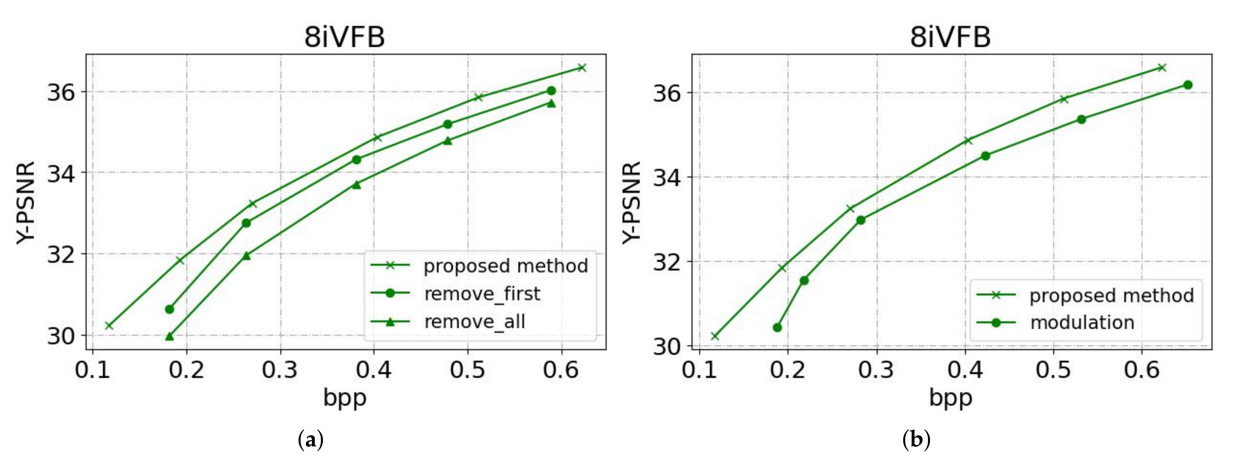
To further make clear the contribution of the introduced NLAM, we set different configurations of network in terms of NLAM. The internal mask branch of NLAM pairs is gradually removed and the network is retrained for performance evaluation. Other experimental conditions remain unchanged and the result is shown in
Figure 9a.
Removing the mask branches of the NLAM pair in the shallow layer in the main encoder-decoders (referred to as “remove_first”) yields a PSNR drop of about 0.3 dB compared to the orginal setting at the same bit rate. The drop is further enlarged when all NLAM pairs’ mask branches are removed (a.k.a., “remove_all”), resulting in a network without any non-local characteristics explorations.
4.4.2. Influence of Variable Rates Modulation
A variable rates compression model is required for practical application, without retraining the model for individual rates. Since the original feature maps are changed by the modulation network in a nonlinear way, the data distribution may change, disturbing the entropy modeling.
Figure 9b shows the comparison result of the proposed method and the one adding modulation (referred to as “modulation”). As we can see in
Table 2, although there is some performance loss, the number of parameters of the model has been significantly reduced, which is critical for applications.
5. Conclusions
In this paper, we propose an end-to-end learned point cloud attribute compression method with non-local attention optimization and a modulation network achieving variable rate compression. The proposed method achieves state-of-the-art performance compared with other existing learning-based methods, in terms of coding performance measured by BD-rate. When compared with traditional compression methods, the proposed method achieves a large improvement over TMC13v6 and further narrow the gap between the state-of-the-art TMC13v14. Specifically, for the BD-rate, the proposed method outperforms TMC13v6, Deep-PCAC and SparsePCAC by 31.5%, 50.7% and 6.3% reduction, respectively, and reduces the gap with TMC13v14 to 29.3%. For practical applications, the variable rate compression model is achieved to overcome the limitation of storing one network per bitrate. In future work, we would like to utilize the geometry information of the point cloud to extract the latent features of the attribute more reasonably and further optimize the corresponding distribution model.


