Object Composition Identification by Measurement of Local Radio Frequency Magnetic Fields with an Atomic Magnetometer

Abstract

Proof of principle of object composition identification based on inductive measurements with an atomic magnetometer has been demonstrated in highly engineered laboratory conditions. Progress in the development of portable miniaturised magnetometers has encouraged on the parallel development of the measurement technologies involving this sensor, in particular concepts that would enable operation in complex test scenarios. Here, we explore the problem of material identification in the context of measurements performed with variable distance between the object and the primary radio-frequency field source and sensor. We identify various aspects of the measurement affected by variable distance and discuss possible solutions, based on the signal phase analysis, a combination of frequency and angular signal dependencies and the implementation of a pair of excitation coils.

1. Introduction

Radio-frequency (rf) atomic magnetometers are an attractive measurement platform for applications ranging from explosives detection [1] and geomagnetic surveys [2,3] to communication [4,5]. They offer the advantage of high sensitivity (fT Hz${}^{-1/2}$ range) [6,7], combined with a wide spectrum of sensor functionalities and can be miniaturised.

Atomic magnetometers are particularly well suited to inductive measurements due to their tunability and the ability to operate at low frequencies [8] that benefit specific measurements schemes such as defect detection [9,10], object surveillance and material identification [11,12]. The problem of material identification plays a critical role in industrial processes (material sorting and quality monitoring) and the security sector (object surveillance). Current methods such as spectroscopic techniques (X-ray Positive Material Identification [13], nuclear magnetic resonance, and mass spectroscopy) are highly accurate and advanced technologies, but require direct access to the object or collection of a sub-sample for analysis. Material identification via inductive measurements provides a non-contact non-destructive testing (NDT) method for remote or portable monitoring.

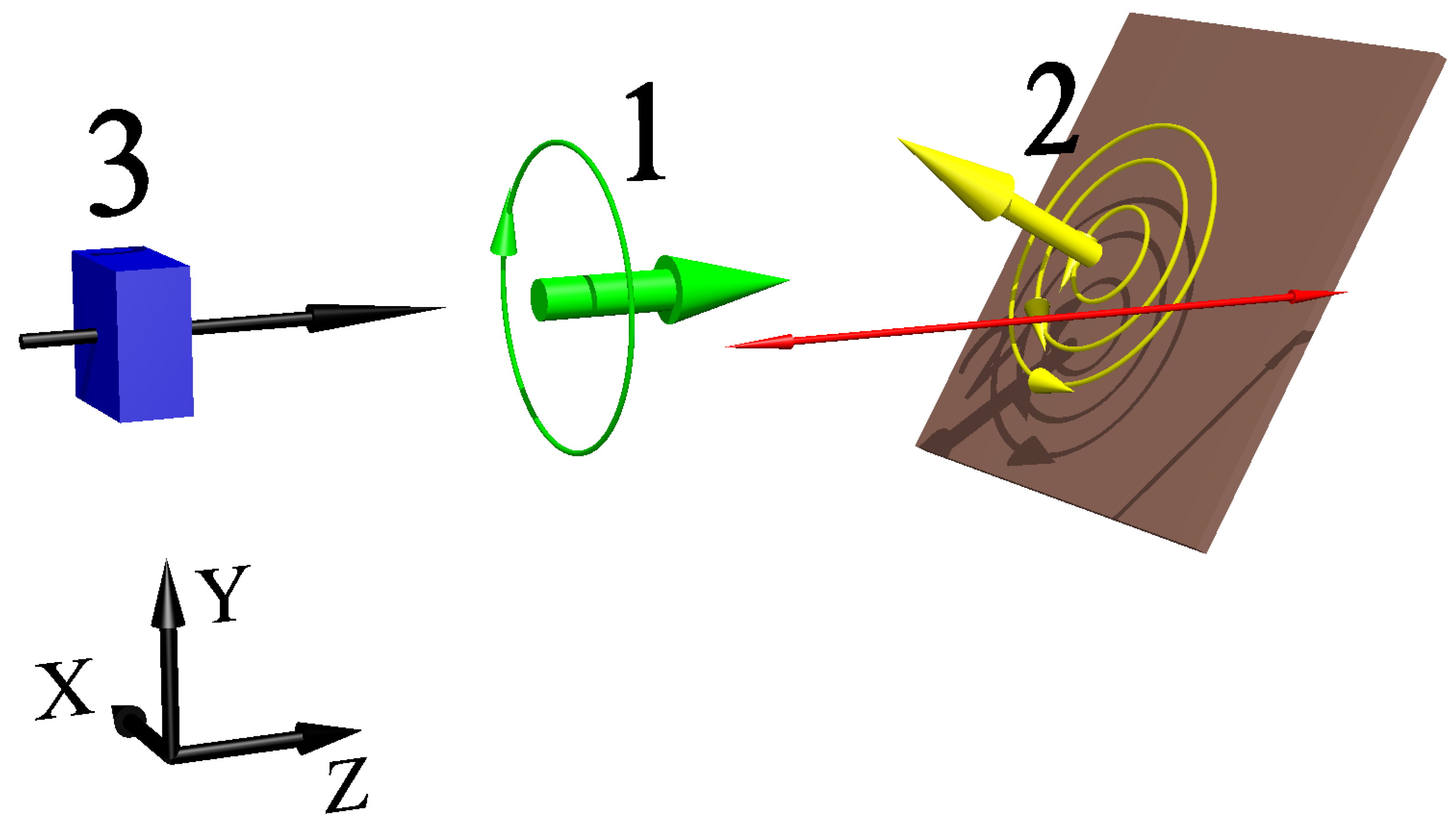
Because of the different terminology present in the literature, we begin with a clarification of the terms used in this paper. We define our experiment as an inductive measurement where an oscillating rf field (primary rf field) creates a response in the object (secondary rf field), which is directly measured by the magnetometer, Figure 1. Although the mechanism of the object response generation is complex, e.g., it is dominated by eddy currents in materials with high electrical conductivity and low magnetic permeability, or by magnetisation in materials with the opposite characteristics, we refer to the measured response (secondary field) as an inductive signal. It should be pointed out that the variety of terminology used in this field accounts for the different aspects of the signal generation, e.g., eddy currents imaging [11], electromagnetic induction imaging [14], or magnetic induction tomography [15]. The range of magnetic field frequencies used in our experiments spans between $4\mathrm{kHz}$ and $40\mathrm{kHz}$, which fall in the ultra-low and very-low radio frequency range. For simplicity, we refer to these values as radio frequencies.

In one of the first realizations of an inductive measurement with an atomic magnetometer, it was demonstrated that the frequency dependence of the inductive signal could facilitate the identification of object composition [11]. This measurement was enabled by the wide tunability of the magnetometer’s operating frequency without compromising measurement sensitivity [8]. Although the demonstration was performed with materials with negligible magnetic permeability, this scheme can be expanded, e.g., as shown in this paper, to all categories of objects that produce inductive signatures.

It has been shown that the result of inductive measurements depends on the relative orientation of the object and primary field direction [12], as illustrated in Figure 1. This is a consequence of the dominating surface character of the response created by eddy currents, even at relatively low operating frequencies, and the volumetric character of the response produced through object magnetisation. The problem was addressed by limiting observation to the component of the secondary field orthogonal to the primary field direction, demonstrating the successful identification of electrically conductive and magnetically permeable objects. These measurements were made possible by the presence of an insensitive sensor axis, enabling easy monitoring of the rf field components orthogonal to the primary field direction [10].

Recently, we demonstrated two object identification scenarios based on implementing the atomic magnetometer in an active feedback loop (so-called spin maser mode) [16]. The spin maser mode brings the benefit of high measurement bandwidth and the ability to track changes in the ambient magnetic field, removing the need for field stabilisation. The results presented here were recorded in the free-running mode (external drive for primary field), with active field stabilisation.

Progress in the development of inductive measurement technology with the rf atomic magnetometers is complemented by the development of important aspects of the measurement, such as; the stabilisation of the bias magnetic field that defines the magnetometer operating frequency [17]; and the sensor components, i.e., silicon wafer vapour cells [18], miniaturisation of laser systems using Vertical Cavity Surface Emitting Laser diodes [19], and sophisticated magnetic coil designs that allow miniaturisation of the measurement unit [20]. Optimisation of the individual components of the magnetometer progresses the instrument towards more practical, real-life usage as opposed to lab-based operation. This increases the importance of studies that identify the technologies measurement limits, determining its commercial viability.

While monitoring the angular dependence of the inductive signal discussed in ref. [12] addresses the problem of the relative orientation of the object and the primary field direction, another layer of complexity is set by possible variation of the distance between the object and the primary field source (lift-off, marked with a red arrow in Figure 1). In this paper, we identify and discuss issues related to variable lift-off and suggest possible solutions to this problem based on the combination of the different magnetometer functionalities.

The complexity of material identification introduced by the variable distance between the primary field source and object is not only limited to the change in field strength. In more general terms, it amounts to a problem of how the amplitude and spatial distribution of the primary field impact the outcome of the measurement. We are going to identify different aspects of this issue in the first part of the paper and point out practical implications.

The second part of the paper explores three possible solutions, that address the issue of variable lift-off, (1) monitoring of the object’s signature phase, (2) frequency dependence of the angular scans, and (3) implementation of more than one source of the primary rf field. The first concept is based on the immunity of the signal phase to lift-off change, while others rely on the evaluation of the lift-off value from the measurement’s output. Our aim is not to provide specific measurement procedures but to point out the observables that contain the essential information for object composition identification in complex test scenarios, i.e., ones that include variable relative orientation between object and the sensor and variable lift-off.

In most cases discussed in this paper, we concentrate on ‘local measurement’, which we define as an inductive measurement performed at a single location, e.g., the centre of the object of interest. The signal readout at a single position could be performed relatively quickly, between tens of milliseconds and a couple of seconds, which allows on-line operation of the detection system (e.g., integrated into a continuous process such as a conveyor belt). As shown in ref. [12], the information regarding object composition could be also acquired by recording 2D (XY) inductive amplitude and phase images. This would be relevant to off-line inspection triggered by the positive result of an on-line test.

2. Materials and Methods

The operation of the rf atomic magnetometer relies on the optical detection of couplings between neighbouring Zeeman sublevels of an atomic ground state generated by an oscillating rf magnetic field. Measurement output, i.e., inductive signal, reflects changes in the amplitude and phase of the rf resonance produced in atoms mainly by the secondary rf magnetic field. The rf spectrum is created by monitoring of the magnetometer signal as the rf field frequency is scanned across the magnetic resonance. Details of the signal generation could be found elsewhere [10,21], here we recall the major parts of the experimental setup. The experiment instrumentation consists of three separate parts: the sensor (rf atomic magnetometer labelled as (3) in Figure 1), the object (2) on a 2D (XY) translation stage, and, the primary rf coil (1) that has a variable lift-off (Z). The rf atomic magnetometer consists of a paraffin-coated caesium atomic vapour cell, two laser beams to interact with the atoms and detection optics/electronics for signal readout, Figure 2a. The volume of the roughly cubic vapour cell is $1{\mathrm{c}\mathrm{m}}^3$ and defines the sensing volume. The cell is at ambient temperature (stabilised at $21{}^{°}\mathrm{C}\pm 1{}^{°}\mathrm{C}$ by the laboratory air conditioning) and in a static magnetic bias field created by tri-axial square Helmholtz coils (side lengths of $1\mathrm{m}$, $0.94\mathrm{m}$, and $0.86\mathrm{m}$). These coils are used with a proportional–integral–derivative (PID) feedback control loop to stabilise the magnetic field (all three axis) that is measured at a fluxgate (three axes Bartington Mag690) close to the cell. PID settings are chosen to also remove $50\mathrm{Hz}$ electronic magnetic field noise. The magnitude of the bias magnetic field defines the rf (Larmor) resonance frequency of the caesium atoms. A circularly polarised laser beam directed along the bias field, called the pump beam, creates a population imbalance within the ground state of the atomic energy levels, polarising the atomic spin states along the bias magnetic field. The beam is locked to the $6{}^2$S${}_{1/2}$ F = 3$\to 6{}^2$P${}_{3/2}$ F${}^{\prime }$ = 2 resonance transition ($D_2$ line, $852\mathrm{n}\mathrm{m}$) and pumps atoms into a stretched state of the F = 4 ground state level, Figure 2b.

Transfer of the atoms is achieved by so-called indirect pumping, which combines strong resonant pumping within the F = 3 level through the $6{}^2$S${}_{1/2}$ F = 3$\to 6{}^2$P${}_{3/2}$ F${}^{\prime }$ = 2 closed transition, spin-exchange collisions that replicate the F = 3 population imbalance in the F = 4 level, and transfer of the population from the F = 3 to F = 4 level through the off-resonant $6{}^2$S${}_{1/2}$ F = 3$\to 6{}^2$P${}_{3/2}$ F${}^{\prime }$ = 4, 5 transitions. Indirect pumping simultaneously addresses two aspects relevant to the magnetometer performance: (1) it depletes the F = 3 level, so that more atoms can contribute to the signal, (2) it creates a high degree of orientation within the F = 4 level without direct optical coupling, which both reduces the width of the rf resonance and increases the signal-to-noise ratio.

An rf magnetic field resonant with the Larmor frequency and perpendicular to the bias field creates atomic coherences within the F = 4 manifold that couples to the linear polarisation of the second laser beam, called the probe beam, through the Faraday effect [22]. The probe beam propagates perpendicularly to the pump beam and bias field and is $2.75\mathrm{GHz}$ red detuned from the $6{}^2$S${}_{1/2}$ F = 3$\to 6{}^2$P${}_{3/2}$ F${}^{\prime }$ = 2 transition. The modulation of the probe beam’s polarisation is detected by a polarimeter, consisting of a polarising beam splitter whose outputs are coupled to a balanced photodetector. This signal is monitored with a lock-in amplifier, that is referenced to the frequency of the primary and secondary rf magnetic fields. The quadrature outputs (X and Y) of the lock-in can be used to calculate the amplitude of the signal ($R=\sqrt{X^2+Y^2}$) and its phase ($\varphi =arctan[Y/X]$), which is directly proportional to the amplitude and phase of the rf field. Magnetometer sensitivity is limited by atomic projection noise and quantum back action at the level of $50{\mathrm{fTHz}}^{-1/2}$ [21]. The bandwidth of the sensor is limited by the atomic response rate at $40\mathrm{Hz}$.

The primary rf field is generated by a coil with a length of $9\mathrm{m}\mathrm{m}$, with a winding thickness of $0.5\mathrm{m}\mathrm{m}$ wound around a ferrite core of $2\mathrm{m}\mathrm{m}$ diameter and $15\mathrm{m}\mathrm{m}$ length. The coil is located in between the object and the vapour cell to represent a realistic measurement geometry. The axis of the coil is directed along the bias magnetic field and centred with the cell to minimise the contribution of the primary field in the measurement [4]. In this configuration, the sensor is most sensitive to the presence of the secondary field generated by the presence of the object, i.e., zero signal recorded when there is no object [10]. The amplitude of the primary rf field generated by the coils varies with the operating frequency due to the frequency-dependent impedance of the coil, and frequency dependence of amplifiers used in the electronics. The data presented and discussed in this manuscript has been calibrated against this variation.

3. Results

3.1. Problem Statement

In real-world applications measurement conditions will likely vary between tests and there will be incomplete object information, i.e., its position (XYZ)/surface geometry, curvature, and orientation. Although we focus on a ’local’ measurement, i.e., inductive measurement performed at the single point (XY) over the object of interest, measurement output depends on all these factors.

A change in lift-off, i.e., object’s position along Z axis, affects the measurement in two distinct ways. Firstly, the strength of the primary field is related to the distance from the coil as described by the Biot–Savart law. The secondary field amplitude is directly proportional to the primary field. Hence, without prior knowledge, a change in lift-off during the measurement may obstruct the proper interpretation of the test outcome. Secondly, magnetic fields diverge away from their source. Divergence length scales are related to the coil geometry, with the field from smaller coils diverging quicker over short distances relative to larger coils. The consequence is the effective integration area of the measurement (resolution) changes with lift-off. The object’s geometry will also influence induction with the primary field. The curvature of the object’s surface and its orientation relative to the primary field influence the distribution of the primary field across its surface. To adequately perform material identification, the influence these parameters have on the measured secondary field must be understood. This section discusses the problems created by variation in lift-off, in the context of composition identification measurements. We present results for objects that are square plates. Discussions will be extended to different geometries where relevant.

3.1.1. Proof of Principle with Fixed Lift-Off

We demonstrated previously that identification of the object composition could be performed through analysis of the angular dependence of the inductive signal produced by the studied object [12]. The concept of angular scanning is important for understanding the results reported in this paper. Below, we summarize the essential elements of this concept and highlight aspects crucial to further analysis. Figure 3 is a plot of (a) amplitude and (b) phase of the rf signal measured over the centre of a $38\times 38\mathrm{m}{\mathrm{m}}^2$ plate made from copper (red diamonds), stainless steel (blue triangles), and ferrite (black squares) as each plate is tilted from $\pm {30}^{°}$. Additionally, all recordings were done at an operational frequency of $6\mathrm{kHz}$. The ferrite plate is $2\mathrm{m}\mathrm{m}$ thick, while the others are all $0.5\mathrm{m}\mathrm{m}$. These measurements were done with a $3\mathrm{m}\mathrm{m}$ lift-off and each point represents the mean of 30 readouts of amplitude and phase of the rf resonance (for a $1\mathrm{s}$ scan time) where the error bars represent one standard deviation. The particular choice of the material is done to illustrate different aspects of the secondary field generation. In particular, the presence of the angular dependence of the signal amplitude, Figure 3a, indicates that the inductive signal is produced in the vicinity of the object’s surface. This is a direct consequence of the dissipative character of the eddy currents generation. We interpret the negligible angular dependence of the secondary field observed in the case of ferrite plate as a result of magnetisation created within the whole volume of the object, generating a field parallel to the primary field (i.e., invisible to the sensor) and partially uncoupled to object orientation. We refer to these two different aspects of the generated signal as surface (eddy currents) and volume (magnetisation) components of the secondary rf field. Consequently, the gradient of the angular dependence of the inductive signal amplitude represents a measure of the ratio between these two components (zero gradient, only volume component; non-zero gradient, non-zero surface component). It needs to be added that at low primary rf field frequencies, i.e., when the skin depth is significantly bigger than the object thickness eddy current generation has at least partially volume character. In summary, the signal observed at a particular angle primarily depends on the electrical conductivity of the object and the primary rf field frequency.

3.1.2. Local Measurements with Variable Lift-Off

Demonstration of the material identification through the amplitude angular dependence was done through measurements at a fixed lift-off [12,23], i.e., with all objects being the same distance from the primary rf coil. Figure 4 shows angular dependencies of the rf signal amplitude (a) and phase (b) recorded over the copper plates with lift-off values of $3\mathrm{m}\mathrm{m}$, $10\mathrm{m}\mathrm{m}$, $20\mathrm{m}\mathrm{m}$, and $30\mathrm{m}\mathrm{m}$. Without prior knowledge of the measurement conditions, i.e., in this case lift-off values, the results of the rf signal amplitude measurements might be interpreted as objects with different compositions.

3.1.3. Change of the rf Signal with Lift-Off

To gain further insight, we measured the dependence on lift-off of the signal amplitude, Figure 5a, and phase, Figure 5b, for a square copper plates with side length of $40\mathrm{m}\mathrm{m}$ (blue solid line), $20\mathrm{m}\mathrm{m}$ (orange dashed line), $8\mathrm{m}\mathrm{m}$ (yellow dotted line), and $4\mathrm{m}\mathrm{m}$ (purple dash-dotted line). The data were recorded with plates angled at ${30}^{°}$, while the black line represents the signal amplitude measured over a plate at $0^{°}$. All amplitudes measured at $0^{°}$ are at the same level for all plate sizes but only one data set ($40\mathrm{m}\mathrm{m}$ plate) is shown for clarity. These plots show that there is a decay in the measured rf resonance amplitude with increasing lift-off. This is due to the decrease in the primary field amplitude at the surface of the plate with increasing lift-off. In addition, at a single lift-off, i.e., $2\mathrm{m}\mathrm{m}$, the measured amplitude increases linearly with plate side length. The reason for this is more complex. The signal measured at the magnetometer reflects the strength of the secondary rf field, but is also related to the change in the spatial distribution of the primary field. The distribution of the primary field will change if it couples inductively to an object, i.e., field lines will deviate relative to the case where there is no object. This results in the generation of a horizontal component of the primary field. Larger objects will disrupt the field distribution more, which leads to an increase in the measured signal amplitude with plate size. Plate size will also influence the secondary rf field through the circumference of the secondary field generating eddy currents, i.e., for the same eddy current density a small circumference imposed by a small plate will result in a smaller field measured at the cell (Biot–Savart law). For the coil and plate sizes used here, this is expected to be a small contribution.

3.2. Object Composition Identification with Local Field Measurement

As shown in the previous subsection, each composition identification test based on local inductive measurement with an unknown relative orientation should address the angular dependence, i.e., monitor the change in the inductive signal as a function of the angle between the object’s surface normal and the insensitive axis (sensor and the primary rf field coil axes). Below, we discuss three ways the problems of relative orientation and variable lift-off could be addressed: (1) monitoring of the object’s phase signature, (2) frequency dependence of the angular scans, and (3) implementation of more than one source of the primary rf field.

Phase

Figure 4b shows the dependence of the phase of the rf signal as a function of the angle between the object’s surface normal and the sensor axis recorded for copper plates with different lift-off values. In contrast to the amplitude data set in Figure 4a, the angular dependence of the signal’s phase show consistency regardless of the lift-off value. For small angles there is a small correlation between measured phase and lift-off, but phase converges to the same value at larger angles, e.g., $\pm {50}^{°}$. A similar trend is confirmed by the results recorded for different object shapes (not shown), and dimensions, Figure 5b. All data sets indicate that the phase of the inductive signal contains information unique to the object’s composition that is immune to a change in lift-off and the object’s dimensions. This statement could be made more general, i.e., the secondary rf field phase values and their distribution over the object do not vary with lift-off value, to include cases of the magnetically permeable objects. This is particularly well illustrated by the inductive images of the ferrite plate, which also indicates some limitations of the phase measurement.

Figure 6 shows a series of amplitude (a) and phase (b) images of the ferrite plate recorded at $0^{°}$ deg with different lift-off values. As discussed in ref. [23], the surface of the ferrite plate (negligible electric conductivity and high magnetic permeability) does not create an observable signal and only generates a non-zero signal around the plate edges. The amplitude of this signal decreases with increasing lift-off. The phase image has the form of a vortex, which reflects the change of the secondary field orientation inside and outside the plate [10,12,23]. The phase images recorded for different lift-offs not only share the same generic pattern (vortex) but also the value of the phase recorded over the same part of the plates are equal for all lift-offs. As shown in ref. [23], the phase image of a magnetically permeable object does not vary with relative orientation between the object and the sensor. To some extent the same property, phase saturation limited angle r ge, e.g., from $+{30}^{°}$ to $+{15}^{°}$ in Figure 3, was also demonstrated for electrically conductive objects. While these two observations prove that the phase is immune to variation of these two important factors in the inductive measurement (relative orientation and lift-off), the accuracy of phase measurement deteriorates with the decrease in signal’s amplitude associated with increasing lift-off. To quantify this statement we use data from Figure 6. We define signal amplitude as an averaged signal along the plate edge. Figure 7a shows a decrease of this amplitude with increasing lift-off value. To demonstrate the phase dependence on the lift-off we average values along the radius of the vortex. Figure 7b shows these phase values averaged along different directions as a function of the lift-off. While the data set confirms that the phase does not change with lift-off, the accuracy of the phase measurement represented by the standard deviation deteriorates with decreasing signal amplitude. The relatively small lift-offs studied in this paper results from using a small primary rf field coil (outer diameter of $3\mathrm{m}\mathrm{m}$) in our experiment. A bigger coil or a coil array might be used to increase the achievable lift-off [24,25]. Similar behaviour, i.e., increasing phase uncertainty has been observed in the same measurement with a copper plate, i.e., electrically conductive object.

3.3. Frequency Dependence of the Angular Scan Gradient

As we have shown in the previous subsection and will show here, the phase of the rf signal in some cases does not contain enough information to make object composition identification. However, combining measurements of the angular dependence and frequency dependence of the rf signal amplitude allows estimation of the lift-off value and subsequently material composition identification.

Recording the full angular variation of the inductive signal is time-consuming and might be impractical in some scenarios. Instead, because of the linear character of the signal’s angular dependence, we use the absolute value of the gradient of this dependence that could be evaluated, in principle, based on only two measurements.

Figure 8 shows the gradient of the angular amplitude dependence as a function of the operating frequency recorded for copper, aluminium, brass, and steel plates recorded at a lift-off of $3\mathrm{m}\mathrm{m}$. It is worth pointing out that each point on this plot represents an object-orientation independent measurement of the signal amplitude at a given frequency. For frequencies higher than $17.5\mathrm{kHz}$ all data sets show a linear dependence on frequency (linear fits indicated with dotted lines). This linear dependence represents the scenario when the object response has a purely surface character, i.e., the skin depth is smaller than the object thickness, and the increase of the signal comes from the frequency dependence of Faraday’s induction. This dependence is generic across all materials, which is reflected in the parallel slopes above $17.5\mathrm{kHz}$. For the frequencies below $17.5\mathrm{kHz}$ for the sets representing copper, brass and aluminium there is a departure from linear dependence. This is caused by the change of character of eddy currents generation, i.e., transition from purely surface to volume generation. In other words, a decrease in efficiency of Faraday induction with decreasing frequency is compensated by the increase of the object volume that contributes to the secondary field generation. The value of the frequency where this change is observed is defined by the ratio between skin depth and object thickness. Steel shows slightly different characteristics than the others. It has the lowest conductivity, which accounts for the reduced gradient (due to smaller secondary field amplitude), but also the smallest skin depth due to its permeability. This results in the extension of the linear character of the gradient’s frequency dependence at low frequencies. It is important to stress, that we observe a non-zero gradient at low frequencies where the skin depth is bigger than the thickness of the object, i.e., at $4\mathrm{kHz}$, because there are still eddy currents circulating on the object’s surface. As discussed in ref. [12] the actual value of the gradient is defined by the ratio between surface and volume generated components of the secondary field.

The distinction between volume and surface characteristics of an object response provides a better understanding of the phase measurement in the context of composition identification. In the high-frequency regime (above $17.5\mathrm{kHz}$, for the data set presented in Figure 8) the secondary field has purely surface character, i.e., it is orthogonal to the surface as shown in Figure 1. Our results confirm that the signal phase generated by materials with high electric conductivity, e.g., copper, aluminium, brass is the same, although still significantly different from that produced by objects with high magnetic permeability, e.g., ferrite as in Figure 6. The phase measurement provides the best discrimination between different object compositions in the low-frequency region, where it shows the highest sensitivity to electric conductivity and magnetic permeability of the object.

Figure 4a shows that the gradient of the inductive signal angular dependence decreases with lift-off. For each lift-off, the same frequency dependence of the angular scan, as shown in Figure 8, was recorded. Based on these results, we extract the gradient of linear frequency dependencies as a function of the lift-off value. Figure 9a shows that these gradient values decrease with the increasing lift-off in the same way for all materials (some of the points overlap). The red dotted curve is an exponential fit to the copper data describing the decay in the primary field at the object with lift-off. The dependence as represented in Figure 9a could be used to calibrate the detection system, and subsequently, the gradient of the linear part of the angular scans frequency dependence shown in Figure 8 could be used as an estimation of lift-off. While the gradient of the high-frequency part of the frequency dependence provides an estimation of the actual distance between the object and the primary rf field source, the offset of this dependence is indicative of the skin depth to object thickness ratio, Figure 9b. It is worth pointing out that, as a consequence of the decreasing signal amplitude, the dynamic range of the offset variation decreases with increasing lift-off. To summarise this part, object composition identification with arbitrary relative orientation and lift-off would require initial calibration of the system, i.e., measurement of the angular gradient’s frequency dependence, Figure 9a, and calibration of the offsets for a few lift-off values, Figure 9b. Actual testing of the object through local measurement of the frequency dependence of angular gradient might be combined with phase measurement at a low operating frequency. Changing the operating frequency of the atomic magnetometer through adjustment of the bias field is relatively straightforward and was already demonstrated in the case of continuous and selective tuning [4].

3.4. Multi-Coil Arrangement

The issue of variable lift-off could be eliminated from the object’s composition identification challenge by the implementation of a multi-primary rf field coil arrangement. Previously, we have shown that primary rf field coils located on opposite sides of the object with either the same or opposite phases produce an inductive image that could also be used for material identification [23]. In particular, we demonstrated that the inductive image of the tilted object located in the centre between two coils has a homogeneous character in contrast to the image recorded with a single coil. Departure from this central location will introduce inhomogeneity in the inductive image and enables estimation of the object lift-off. Here, the focus is on local measurements and lift-off estimation would be based on a comparison of the outputs of local measurements performed with excitation by a single coil on either side of the object and with the same two coils in phase acting simultaneously with each other.

Figure 10a shows the amplitude of the rf signal as a function of the angle between the normal to the object surface and the sensor axis recorded for copper plates with excitation produced by a single coil on the same (navy diamonds)/opposite side (red triangles) of the plate with respect to the sensor and the set of two coils ((green points). The distance between the primary rf field coils and the object is different by 5 mm, which is reflected in difference in the rf signal amplitudes. We have recorded angular dependencies, as shown in Figure 10a, for different lift-offs values. For all measurements, the distance between the two coils is the same. This could mimic a scenario, where the coils are located on both sides of a conveyor belt (fixed distance), while the individual lift-offs could vary depending on the position of the object on the conveyor belt. As in the previous subsection, we characterise data sets by the gradient of the angular dependence of the rf signal, as an orientation independent measure of the rf signal. Figure 10b shows the gradients of the angular dependence recorded with the single primary rf field coil as a function of the difference in lift-offs measured from the point where the lift-off between each coil is equal. The values of gradients have been normalised to the value recorded in the two coils arrangement. In the particular case of equal lift-offs gradients are equal to 0.5, i.e., signal recorded with a single coil is equal to half of the signal observed with two coils. The dependence of this normalised gradient value recorded with a single coil could be used to evaluate the lift-off, i.e., position of the object with respect to the coils.

As mentioned before the symmetry (or lack of symmetry) in the amplitude might also provide information about the relative lift-off difference. Although we are focusing on local measurement, analysis of the cross-section through the centre of the amplitude image provides insight into the limitation of the method discussed above. Figure 11a shows the amplitude of the rf signal recorded over a $0.5\mathrm{m}\mathrm{m}$ thick square copper plate with an area of $40\times 40\mathrm{m}{\mathrm{m}}^2$ for the two coils configuration (navy triangles) and single coil arrangements (green diamonds and red points). The data were recorded with plates angled at ${30}^{°}$. For equal lift-offs, the signal recorded in two coils arrangement is symmetric. Because of the plate tilt, the signals recorded in the single coil configuration are asymmetric and the maximum amplitudes recorded in both cases are nearly equal (the difference comes from imperfection in coils alignments with respect to the bias magnetic field). The method discussed in the previous paragraph referred to measurements conducted at the centre of the plate. The data shown in Figure 11b confirm that the amplitudes recorded only at this point with the single coil arrangement are equal (blue diamonds, and red triangles), when each coil has the same lift-off. However, the general behaviour of the rf signal recorded at any location over the plate is still valid. Figure 11a,c shows the same signal dependencies when recorded with different lift-offs, e.g., Figure 11a where the lift-off for the coil on same side as sensor is (red triangles) and the opposite coil is (blue diamonds). The data confirm that in these cases all dependencies show asymmetries and the maximum values recorded in single coil arrangements are not equal. It also shows that difference in the signal recorded in any location is minimised for the case of the equal lift-offs.

4. Conclusions

In the process of developing a concept from proof of principle to a complete instrument, it is important to address real-life measurement complexities, which have been avoided in the initial stages when evaluating the feasibility of certain aspects of the technology. Here, we presented possible options to address the issue of variable orientation and lift-off in object composition identification based on inductive measurement with an rf atomic magnetometer.

Our approach relies on the ability to identify the surface vs. volumetric character of the secondary rf field generation through the signal’s angular dependence. Essentially, it is a consequence of our measurement strategy where we concentrate on the secondary field components orthogonal to the primary rf field. The ability to determine the character of the secondary field combined with the signal’s frequency dependence allows selective operation of the frequency range where the object response produced by eddy currents has purely surface character regardless of object composition. Identification of composition independent variables enables calibration of the detection system, estimation of the lift-off value for each measurement and subsequently material identification. Measurements of the angular and frequency dependencies of the rf signal might be complemented by the implementation of a set of the primary rf field coils that enables independent evaluation of the lift-off. Subsequent object composition identification was performed for objects with the same geometry, future work will study the signal response for different geometries.

While concentrating on the development of a measurement toolkit we recognise that actual implementation of the discussed techniques, e.g., operation with lift-off at 50–100 cm range, requires the development of dedicated hardware, e.g., rf field sources and portable detection systems. The works towards this goal are underway.