Abstract
This work provides a feasible solution to the shipborne short landing problem for thrust-vectoring V/STOL vehicles. The short takeoff and shipborne rolling vertical landing strategy was designed in this work. First, the strategy design reference was established by flying performance and mission requirements, including the short takeoff and landing performance, deceleration performance, trajectory stability, velocity stability, and conversion corridor, using attainable equilibrium set methods based on the six dimensions of freedom model of the study object. Then, a piecewise short takeoff landing strategy was designed based on the references, together with a nonlinear dynamic inverse-based control designed frame for strategy execution. Finally, the hardware-in-loop Monte-Carlo simulation was implemented for the strategy feasibility verification. The proposed short takeoff and landing strategy satisfies the shipborne short takeoff and landing mission requirements. The short takeoff shortens the taxiing distance by 40% compared to a normal takeoff. With a 20% perturbance on all model parameters, the touchdown speed can be controlled to 14 ± 1 m/s, and the landing point position can be constrained inside a 5 m radius circle with almost zero lateral displacements.
1. Introduction
In the military, stealth performance dominates aerial vehicle designs due to the successful practice of the B-2 strategic bombers in the Gulf War. However, stealth is usually achieved at the price of aerodynamic configurations, which inevitably causes poor takeoff/landing performance [1,2,3]. When it comes to shipborne takeoff/landing, this issue becomes somewhat unacceptable due to the limited runway range. A thrust-vectored aircraft is a resolution to this issue, as the propulsion system compensates for aerodynamic loss and enables the aircraft to perform short or vertical takeoffs and landings [4]. The short takeoff (STO) and shipborne rolling vertical landing (SRVL) is a landing strategy proposed for the thrust-vectored aircraft by the US marines. Even though a manned F-35B execution video is published online, the accessible literature on the systematic SRVL approach is limited.
For the performance requirements, Reference [5] gave the shore and decked verification of the F-35B vehicles, with the performance requirements specified. Reference [6] provided a systematic performance computation method based on the attainable equilibrium set methods. For the flying quality requirements, Reference [7] designed a dynamic inverse controller for the X-35B, which is the predecessor of F-35B, and verified the flying qualities of the closed-loop system. The hover state directional guidelines were given, but the left procedures were not specified, which were verified by Cooper–Harper standards instead. Reference [8] designed H-∞ controllers for helicopters according to robust flying qualities, which may provide some reference for hovering state flying quality. Reference [9] gave the longitudinal results of the flying quality analysis of an F/A -18 fighter equipped with the JAS 39 mini-stick controller, but the Cooper–Harper ratings were still applied, and no specific guidelines were given. Reference [10] stated: the joint strike fighter projects, which include the F-35B project, use the performance-based specifications instead of the traditional flying quality for controller designs. However, the classical design guidelines such as Mil-F-83300, AGARD 577, and UK DEF STAN 00-970 were also referred to for verification. The limited criterion pushed us to apply the specifications for the normal fighters for control system design.
The research on the control system design for the short takeoff or vertical landing (STOVL) vehicles is comparatively rich. Reference [11] applied the dynamic inverse theory and designed the controller for the F-35B reduced-scale vehicles for the transitional flight control, and the simulation results reflected an excellent tracking performance. Reference [12] used an L1 adaptive [13] inner-loop controller and designed a roll-horizon landing deceleration and landing strategy for the hybrid-wings vehicles. Reference [14] applied the nonlinear active disturbance rejection controller (ADRC) to the tilt wings in the landing stage control. For less maintenance costs and higher reliability, the NDI controller is used by the F-35B projects [2,15]. Since the NDI control theory has been applied in many mature industrial products [16,17,18], this work follows the design. Besides, the allocation issue is crucial for a redundant control system. Reference [19] evaluated the profits of the optimization allocation technics, such as pseudoinverse, quadratic programming, and fixed-point algorithms, and found that even though the tracking error can be reduced most of the time, it is possibly uncontrollable in certain cases. Reference [20] compared the allocation method with the servomechanism method and concluded that control allocation makes the performance uniformly better. For the flight security issue, References [21,22,23] provided an envelope protection method for small unmanned aerial vehicles (UAVs) based on performance boundaries, which inspired us in the parameter boundary setting methods. For the navigation and path-following problems, Reference [24] designed a robust trajectory controller based on an optimal control principle for the thrust-vectoring vehicles. Reference [25] developed a robust trajectory tracking algorithm for normal underactuated aircraft systems based on adaptive linear controllers for the strategy trajectory tracking problems. Reference [26] applied ADRC in line-of-sight angle control in an outer loop and conducted successful trajectory guidance for maneuvering target interception. References [27,28,29] provided the simple but practical Monte-Carlo method for the controller robustness verification for the simulation verification issue.
This paper designs a precise and stable landing strategy for the thrust-vectoring S/VTOL aircraft to satisfy its demand on landing in narrow and dangerous environments, granting a better landing performance under the premise of meeting the flight quality. The context of this work is organized as:
- A brief introduction of the studied F-35B platform, especially its propulsion system and the flight dynamics model for it.
- Performance analyses of the studied F-35B platform based on the flight dynamics model.
- The design of the STO and SRVL strategy based on the performance analysis results and the NDI-based control system supporting the strategy execution.
- The simulation of the whole system to verify the strategy design and the conclusion based on the simulation results.
2. The Platform Modeling
2.1. The Propulsion System
The reduced-scale F-35B aircraft (as shown in Figure 1) adopts the propulsion system composed of the three-bearing swivel ducted (3BSD) nozzle and the lift fan, as shown in Figure 2, and the main parameters are given in Table 1. In the cruise mode, the 3BSD nozzle points backward to provide the forward flight power, while in vertical mode, the 3BSD nozzle deflects 90 degrees downwards with the lift fan activated to generate the required lift together. In the vertical mode, the pitch channel is controlled by the speed of the lift fan and main ducted fan, which provides pitch stability and control efficiency. The roll channel is driven by the two side nozzles, whose airflow is controlled by the roll control mechanism. The yaw channel can be controlled by deflecting the 3BSD vector nozzle in the lateral planes.
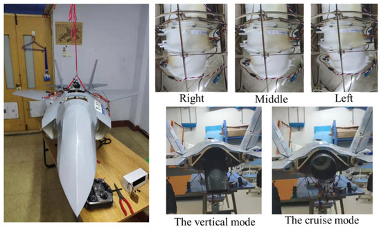
Figure 1.
The reduced-scale F-35B platform.
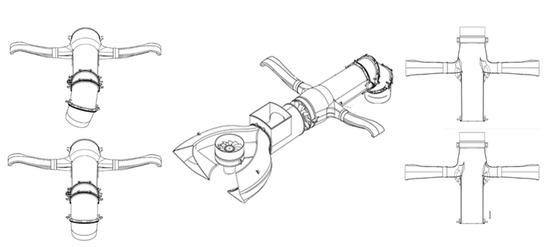
Figure 2.
Power system.

Table 1.
V/STOL main parameters.
2.2. The Flight Dynamics Model
The forces and moments acting on the study object can be classified into three classes:
Class 1: The aerodynamic forces and moments. The forces include the lift, drag, and side force, and the moments include the roll, pitch, and yaw moments. All these forces and moments are measured in wind tunnel tests.
Class 2: The forces and moments due to propulsion system that is introduced in Section 2.1.
Class 3: The gravity.
The forces and moments of the three classes are then projected to the body frame of the F-35B model and subjected to the 6-DOF function of motion to calculate the derivatives of the motion states, such as position displacements and angular rates, and the state space model of the F-35B system can be acquired.
3. Performance Analysis
The suitable STO and SRVL strategy formation requires suitable and specific references for parameter specification. Flying performance is the basic criterion since the performance boundaries reflect the capability of the vehicle. This work builds the performance boundaries that involve short takeoff and landing, deceleration performance, velocity and trajectory stability, and the conversion corridor based on the 6-DOF model of the reduced-scale F-35B protype using AES methods [6].
3.1. Short Takeoff Performance
The utilization of a thrust vector can effectively shorten the takeoff distance. During the takeoff, the takeoff velocity can be efficiently reduced by controlling the thrust vector to provide part of the lift in cooperation with the lift fan. Meanwhile, the reduction in the support force of the rear wheel on the ground reduces the friction resistance and increases the taxiing acceleration so that the takeoff velocity can be achieved in a shorter time and improve the takeoff performance. However, only a part of the thrust vector produces thrust, and this reduces the takeoff acceleration of the vehicle. Therefore, it is necessary to optimize the position of the thrust vector to achieve the shortest liftoff distance.
An airplane takes off in three stages: (1) from the home point to the nose wheel lifting; (2) from lifting its nose wheel until the aircraft lifts off the ground; and (3) lifting off the ground to a safe height. Only two processes (1) and (2) are considered in this section, and the problem is transformed into how to adjust the thrust of the lift fan and the vector deflection angle of the 3BSD to minimize the distance between the home point and the departure point under the condition that the certain takeoff angle is 6° and the 3BSD is working at maximum power.
In this process, the vehicle is subject to aerodynamic force, , the lift fan, , the thrust vector, , gravity, and friction, , and when calculating the takeoff distance through the real-time attack angle,, the real-time aerodynamic force can be calculated by interpolating the drag coefficient, , and the lift coefficient, The lift fan and the deflection angle of the 3BSD, remain constant values for the whole run process, and these two constants need to be determined. Gravity remains the same value. The ground friction coefficient was chosen to be the rolling friction coefficient of a cement floor, and the friction coefficient was chosen to be 0.03. The angle of attack, , remains a certain value of 0.33 degrees in stage 1. During stage 2, the changing rate of the attack angle was chosen to be 2 degrees/s according to the bandwidth of the pitching angle rate loop, which is about 1 rad/s.
The lift fan was chosen to be 30%, 40%, 50%, 60%, and 70% of the maximum thrust, and the aircraft was trimmed to find the deflection angle of the 3BSD, and the takeoff velocity at the maximum thrust vector,. The trimming curve is shown below in Figure 3.
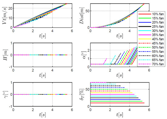
Figure 3.
Time history of lift fan during rolling to take off from the ground.
After trimming processing, the variation curves of the deflection angle of the 3BSD, the throttle of the lift fan, and the trimming velocity are shown below in Figure 4.
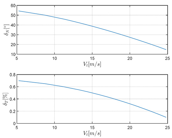
Figure 4.
The variation curves of the throttle of the lift fan and the deflection angle of the 3BSD.
According to the Table 2, the shortest running distance appears when the size of the lift fan ranges between 0.5 and 0.7.
Table 2.
The calculation results of the takeoff performance.
3.2. Landing Performance
To reveal the advantage of the SRVL, this work compares the performances of the SRVL with those of the conventional landing method. The touchdown state boundaries of the two landing methods are calculated for comparison by establishing the attainable equilibrium sets of the controllable flight envelope based on the flight dynamics model established in Section 2.
Principally, the state constraints exist in the attitude angles, flight path angle, and the flight speed, which are given by Equation (1):
where and are the derivatives of the angle of attack and pitch angular speed, and are the pitch angle and its maximum value, is the flight path angle, whose default value is , is the airspeed, is the longitudinal deflection angle of the thrust vector nozzle, and and are its boundaries, which are and in SRVL and and in conventional landing. The calculation procedures are given in the flow chart (Figure 5).
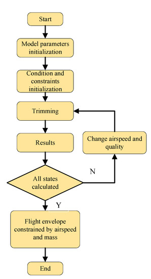
Figure 5.
Landing performance calculation logic.
The lower boundary of the mass is 13 kg, which is the dead load of the aircraft. The calculation lower boundary of the velocity is 0 m/s, and the upper boundary is 25 m/s, which was determined by the runway range and deceleration performance.
The calculation results are given in Figure 6, which shows that when the mass is 13 kg the touchdown speed reduces from 18.5 m/s to 6 m/s if the SRVL is adopted and that if the minimum touchdown speed is fixed the landing load enhances from 13 kg to 20.5 kg. This means that the SRVL may expand the feasible region of touchdown speed and landing load to twice as much as before, which is definitely in favor of landing strategy formulation and flight mission planning.
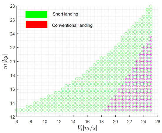
Figure 6.
Touchdown state feasible zone.
3.3. Deceleration Performance
In the deceleration stage, the aircraft are expected to have sufficient velocity control efficiency. The forward flight velocity along the x-axis, , and the descending speed, , and its derivative, , along the z-axis in the ground frame can be acquired by Equation (2):
where and are the thrust vectors of the lift fan and thrust vector nozzle, and are the dynamic pressure and reference area, and are the lift coefficient and drag coefficient, and is tilt angle of the 3BSD. Because the descending rates are commonly controlled by the uniform throttle and the forward flight speeds are controlled by the deflection angle of the thrust vector nozzle, the dynamic functions of the aircraft can be rewritten as Equation (3).
Since the flight path angle is given, the aerodynamic coefficient is approximately a function of the pitch angle, . Once is given, the forward flight speed and descending rate can be calculated with each control input, namely, the thrust and nozzle deflection angle. The results are given in Figure 7.
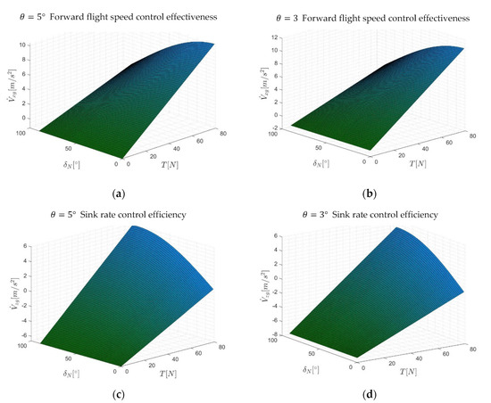
Figure 7.
Deceleration performance analysis diagram: (a) Forward flight speed control effectiveness; (b) Forward flight speed control effectiveness; (c) Sink rate control efficiency; (d) Sink rate control efficiency.
3.4. Trajectory Stability
At the SRVL stage, the flight quality specifies some requirements on the trajectory stability. The level-1 flight quality [6,30] requires that the derivatives of the flight path angle versus the airspeed, , should satisfy , and the difference between airspeed at the minimum approaching speed, , and should be less than . can be acquired by Equation (4).
The trimming points can be evaluated according to the stable gliding constraints set by this work (given in Equation (5)).
where , and, are the yaw angle, roll angle, and sideslip angle, respectively, and and are the pitch angular rate and yaw angular rate.
As the flight path angle determines the gliding speed, given the control inputs, the airspeed satisfying the level-1 flight quality was evaluated by giving different flight path angles and trimming the vehicle. The results are shown in Figure 8, where the region between the red dashed lines and the black dashed line is the level-1 flying quality region, and the green dashed line is . The velocity area of the green dashed line distributed in the level-1 flight quality region is the airspeed ranges stratifying the level-1 flight quality requirement, which is .
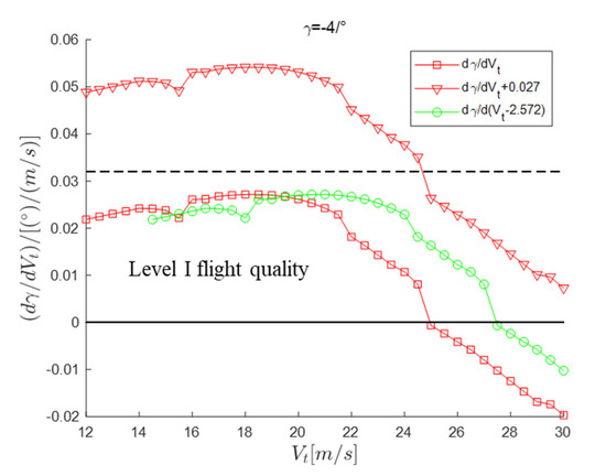
Figure 8.
Trajectory stability analysis.
3.5. Velocity Stability
The aircraft possessing velocity stability have an edge on landing risks. The normal landing aircraft velocity stability criterion is given by Equation (6).
where is the required thrust, and is the dynamic pressure.
Nevertheless, the velocity stability criterion on SRVL is still not published. Thus, this part derives the velocity stability criterion of the SRVL from that of the normal landing.
Equation (7) is satisfied when the aircraft is in a steady straight-level flight.
Thus, Equation (8) is given:
Therefore, the velocity stability criterion can be rewritten as:
For the steady straight gliding, the force analysis function is:
Therefore, compared to Equation (8), the variables used in Equation (9) become:
Since the gliding angle, , is a fixed value set by the users and is usually a small number, equals approximately one and equals approximately zero, that is, and . Therefore, derives from Equation (11) and is almost the same as that derived from Equation (8), as is . This means that the velocity stability criterion is still applicable in the steady straight-gliding case.
For the SRVL case, the propulsion system provides direct lift. Thus, Equation (10) should be adjusted to Equation (12).
where is the direct lift generated by the propulsion system. Now, Equation (11) converts to:
In the steady straight-gliding case, the gliding angle is a constant. When discussing stability issues, the control inputs are all given fixed values, which means the control inputs are constants too. Therefore, the direct lift provided by the propulsion system is also a constant. Then, the derivative of () versus time is still a constant that multiplies the derivative of versus time. To make it clear, . Thus, Equation (9) in the SRVL case turns into:
This means the derivative of the required thrust versus dynamic pressure in the SRVL landing case is what it is in the normal landing case multiplying .
Usually, the direct lift provided by the propulsion system is no more than unless the aerodynamic lift is a negative value. Therefore, the velocity stability criterion of the SRVL case is still Equation (6).
Then, the velocity stability area can be calculated by Equation (6) for each pitch angle. Take the pitch angle of 3 degrees as an example. For a set forward flight airspeed and descending rate, the gliding angle is determined, as are the angle of attack and the aerodynamic coefficients, and . With these parameters, the velocity stability was calculated by the equations deduced above. The results are given in Figure 9a, where the green points are the stable points and the red points are the unstable points. The green points composed the stable region of the flight path angle. The feasible flight path angle was determined for each pitch angle. Piling them together, the flight path feasible zone for the whole flight mission was acquired.
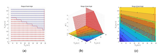
Figure 9.
Track angle analysis diagram: (a) velocity stability analysis; (b) global flight path angle feasible region; (c) comparison of flight path angle feasible region.
It is revealed in Figure 9b that the feasible zone of flight path angles shrinks with the pitch angle increasing. Specifically, the lower boundaries of the flight path angle are plotted in Figure 9c by the blue lines. Obviously, the lower boundaries decrease from to .
The method to establish the strategy parameter boundaries is similar to that to set the transition corridor [31] of multi-mode aircrafts such as composite wings and tilt wings. They all analyze the limiting factors to establish the boundaries and then search for appropriate parameters in the feasible zone. The conventional boundary construction methods treat each limiting factor singly and then synthesize them for a global feasible zone, while the attainable equilibrium set methods systematically think over all the factors and construct the zone directly, which is fairly versatile and robust and not confined to the specific forms of the study objects. However, the boundaries built by AES are not continuous, which costs a high calculation price for precision.
3.6. Transition Corridor
In a complete mission profile, the conversion mode is the process of conversion between the vertical takeoff and landing mode and the fixed wing mode. At this stage, the gravity and drag of the aircraft need to be overcome by the reasonable distribution of the aerodynamic force and power system. However, when flying at a low speed, the required angle of attack may be too large, resulting in a stall. When flying forward at a high speed, it may cause thrust and drag imbalance. Under so many restrictions, the F-35B vehicle can only convert the vertical takeoff and landing mode and fixed wing mode within a certain speed range. This speed range consists of all feasible tilting paths, namely, the tilting transition corridor. The transition corridor is constructed by AES methods. AES is the equilibrium point set that the aircraft can achieve inside the control efficiency boundaries, which is widely used in the controllable boundary establishment of aircrafts. After setting the constraint conditions, the equilibrium boundary can be acquired by trimming the aircraft in all possible states. The calculation procedure is shown below in Figure 10:
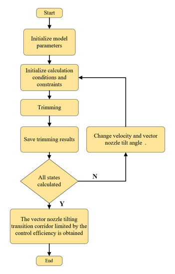
Figure 10.
Conversion corridor establishment logic.
The constraints on the state variables are:
where and are the derivatives of the angle attack and pitch angular rate versus time, and are the boundaries of the angle of attack, and are the velocity components along the body x-axis and z-axis, and and are the true airspeed and 3BSD deflection angles.
Besides, the control input saturation parameters should be given according to the control efficiency, as shown in Table 3:
Table 3.
The limits of the F-35B actuators.
According to the aforementioned constraint conditions, the aircraft was trimmed in all possible states. For those single failure points, they were replaced by their neighbors. The results whose trimming flight path angles, , were over 20 degrees were removed for a smooth transition trajectory. Figure 11 presents the transition corridor. It is reasonable that the left boundary is limited by the tilt angle of the 3BSD nozzle, as the gravity is balanced mainly by the thrust vectors, and the right boundary is limited by the attainable thrust to balance the aerodynamic drag. Having obtained the transition corridor, a straight line was plotted inside the corridor and was chosen as the initial transition trajectory for optimization.
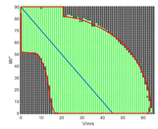
Figure 11.
Conversion corridor of V/STOL aircraft.
4. The STO Strategy
Using the thrust vector can effectively shorten the takeoff distance. When the aircraft takes off, the control of the thrust vector and the lift fan bear part of the lift, which can effectively reduce the takeoff distance. The short takeoff process comprises three stages: (1) from the starting point to the nose wheel lifting; (2) from the lift the nose wheel until the aircraft lifts off the ground; and (3) lifting off the ground to a safe height, as shown in Figure 12.
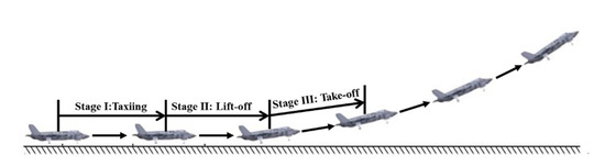
Figure 12.
STO strategy.
- Stage I: Taxiing
In this stage, the altitude and pitch attitude of the aircraft are almost unchanged, and the taxiing speed is parallel to the straight deck. Therefore, the following approximate conditions are met: , , and . Since the engine is at full opening force in this process, a reasonable thrust deflection angle must be set in advance to ensure the short takeoff performance. According to the takeoff performance analysis, we chose a lift fan thrust of 50% and tilt angle of 40°.
- 2.
- Stage Ⅱ: Liftoff
The speed gradually increases to 0.7~0.9 times the ground clearance speed. The pilot controls the aircraft to lift the front wheels and then keeps the two main wheels on the ground to continue to accelerate the taxiing. At this time, the aircraft is still parallel to the runway, and , but starts to increase, and .
- 3.
- Stage Ⅲ: Takeoff
When the speed reaches the ground clearance speed and the vehicle lift is equal to the aircraft gravity, the main wheel of the aircraft leaves the ground and turns to an accelerated ascent. Meanwhile, the ground effect disappears, but as the aircraft leaves the ground, the jet flow is affected by the opposite incoming flow, resulting in the jet-induced effect. This effect is essentially caused by the downward jet flow between the lift fan and the 3BSD and the upward “fountain flow” between them. However, it is generally manifested as the loss of lift and the generation of head-up torque. In addition, considering the thrust vector control characteristics of the aircraft, the lift fan can be turned off and the tail nozzle can be transferred to the normal flight state.
It can be seen in Table 3 that the shortest running distance is between 40~70% fan thrust. In order to obtain accurate optimal results, the batch gradient descent algorithm was used to iteratively optimize the fan value, and the calculation flow chart is as follows in Figure 13 and Figure 14:
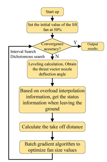
Figure 13.
Optimization algorithm of the shortest takeoff distance.
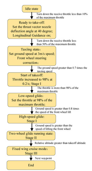
Figure 14.
Control logic of the STO strategy.
The final short takeoff strategy is as follows:
5. The SRVL Strategy
Given the flying performance analyses, the SRVL strategy can be customized. This section designs the piecewise SRVL strategy, and an NDI-based control architecture to support the strategy implementation.
Generally, the SRVL has three in-air stages: the descending and deceleration stage, the stability adjustment stage, and the touchdown preparation stage, as shown in Figure 15.
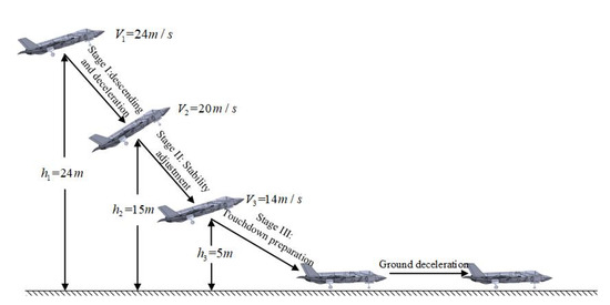
Figure 15.
SRVL strategy.
- Stage I: Descending and deceleration
In this stage, the aircraft enters the landing window from the last cruise way point. As the airspeed is still fairly high, the aerodynamic control surfaces have enough control efficiency for attitude control. Therefore, the aircraft is driven by attitudes for flight path following. For deceleration, the propulsion system is idle to cut off the energy import, and the aerodynamic drag dissipates the kinetic energy. Therefore, in this stage, the thrust vector nozzle can be adjusted for flight mode transition.
The airspeed that divides the descending and deceleration stage and the stability-adjusting stage is named the stage-2 window speed, . If it is set too high, the aircraft will have insufficient time for an attitude adjustment in the stability-adjusting stage, and in the descending and deceleration stage, the thrust vector nozzle has to deflect rapidly for mode transition, which brings about the rapid inertia change. These all increase the risk of controllability loss. However, an under-evaluated may also cause stall and controllability loss. Thus, requires a cautious selection that can be instructed by the aforementioned trajectory stability. In the preliminary design, the flight path angle was set as , and according to the level-1 flight quality specification (analyzed in Section 3.2), the last cruise waypoint speed, which is also the stage-1 window speed, , was set as and .
- 2.
- Stage II: Stability Adjustment
In this stage, the aircraft is required to decelerate from to touchdown speed, , which is also the stage-3 window speed. This work desires to verify the designed controller for its stability augmentation ability. Thus was set as the stall speed, . To acquire enough deceleration efficiency, the pitch angle was assigned a default value in advance for the angle of attack control. The default value was set according to safety landing altitude specifications. Empirically, the stage-2 window altitude, , was set as 15 m, and the stage-3 window altitude, , was set as 5 m, which means that the aircraft was required to decelerate to touchdown speed with the altitude decreasing by less than 10 m. Given the flight path angle , the forward flight range was easily obtained as 143 m. The forward flight speed changed from to , which needs a deceleration of . To let the aircraft be bound to adjust the expected attitude in this stage, a safety margin of 50% was reserved. Thus, the deceleration was required to be . According to the performance analysis in Figure 7, a more than 5 degree pitch angle was required.
- 3.
- Stage III: Touchdown preparation
In the touchdown preparation stage, the descending rate is controlled by the direct lift coming from the thrust vector nozzle and lift fan. The forward flight speed is governed by the backward thrust component of the thrust vector. The descending rate and the pitch angle needed to be set in advance and were designated as and by this work. According to the performance analysis results in Figure 9, it was still inside the feasible zone that when .
Since the stages of the SRVL strategy impact each other on their default states and identification criteria, for a better strategy, the parameters have to be optimized by an iteration algorithm. With the preliminary values, the algorithm will give an optimized solution. The algorithm procedures are illustrated in Figure 16 and the optimized strategy is illustrated in Figure 17.
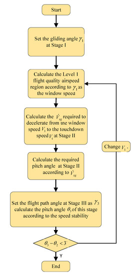
Figure 16.
Optimization algorithm.
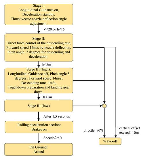
Figure 17.
Control logic of the SRVL strategy.
6. The Controller Design
A control structure was established to implement the aforementioned strategy, as shown in Figure 18 and Figure 19.
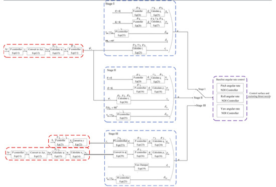
Figure 18.
Control architecture of STO strategy.
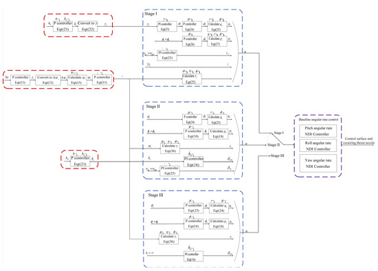
Figure 19.
Control architecture of SRVL strategy.
Clearly, this control scheme is divided into two layers, the outer loop for guidance and the inner loop for stability augmentation. This architecture uses the uniform inner loop, ensuring a consistent stability performance at all stages and executing the strategy control logics by switching the outer-loop control modes.
6.1. The Outer-Loop Design
The inputs of the outer loops are the current position of the vehicle and the desired trajectory, which is typically decoupled in longitudinal and lateral characteristics. The outer loop uses the position information to calculate the desired angular rate and translate them to the inner loop for stability control.
At stage I, the longitudinal and lateral navigation mechanisms are activated for path tracking. The lateral controller uses the cross-track error, , and path azimuth angle, , as the control inputs to calculate the azimuth angle command, .
First, the desired lateral speed is calculated by a simple proportional relation.
Here, is the proportional gain. Equation (16) aims to let the cross-track error converge with a time level of 1/.
The desired azimuth angle, , can be calculated by the desired lateral speed:
where the is the ground speed of the aircraft. Since is usually a small number, approximately, . The range of is limited to . Then, the azimuth angle command is obtained by and as:
Using the direction conversion matrix, the angular speed in the ground frame is converted to the body frame:
According to Equation (19), the yaw angular rate command is given as:
The longitudinal controller uses the desired altitude, , the desired descending or climbing rate, , and the real altitude, , as the inputs to calculate the descending rate command:
where is the proportional gain. Then, the descending rate command is converted to the gliding angle command:
With the proportional-integral control, the pitch angle command is given as:
where is the proportional gain and is the integral gain. Then, can be controlled by a proportional controller:
where is the proportional gain and is the pitch angular rate command.
According to Equation (19), the pitch angular rate can be expressed as:
In the roll channel, the roll angle is controlled by a proportional controller:
where is the proportional gain.
According to Equation (19), the roll angular rate can be expressed as:
In the speed channel, the desired ground velocity, , is controlled by a proportional and integral controller. The input is the real ground velocity of the aircraft, , and the output is the throttle command, .
where is the proportional gain and is the integral gain.
Besides, the deflection angle of the thrust vector is negatively correlated with the ground speed.
All the aforementioned commands construct the inner-loop inputs for stage I, written as .
At stage II, the lateral controller is the same as that in stage I, while the longitudinal controller calculates the descending rate command, , by Equation (21) and then figures out the throttle command of the thrust vector nozzle and the lift fan with :
where is the proportional gain and is the integral gain.
A proportional controller controls the pitch channel:
where is the proportional gain and is the pitch angular rate command.
The desired groundspeed is controlled by the proportional-integral controller in the speed channel. The input is the real ground speed of the aircraft, , and the output is the deflection angle of the thrust vector nozzle:
where is the proportional gain and is the integral gain.
The outputs of the stage II outer loop are .
At stage III, the controllers are the same as that at stage I in all channels. The outputs are also .
6.2. The Inner-Loop Design
The inner loop was designed based on the dynamic inverse theory. First, given the nonlinear rotational function of the aircraft:
where , , are the inertia moments and is the inertia product, , , are the angular rates around the body x-y-z-axis, and , , are the moments around x-y-z-axis, the angular rate can be expressed as:
and
where , , are the moments around the x-y-z axis without control, , , are the control moments around x-y-z axis, respectively, and – are the inertia coefficients given by Table 4.
Table 4.
Inertia coefficients.
It is easy to obtain the inverse matrix of as:
Therefore, the inner-loop controller was designed according to dynamic inverse theory as:
where is the control commands and are the desired angular rates translated from the outer loop.
6.3. The Allocator Design
The inner-loop controller was designed based on the mature dynamic inverse control law, while the control actuators of the STOVL are abundant. A control allocator is necessary for such a system. This work constructed the control allocator based on the control efficiency.
In the low-speed modes, the pitch control moment is generated by the differential speed of the lift fan and the main ducted fan, the roll control moment is given by the differential flow of the two side nozzles, and the yaw control moment is provided by the deflection angle of the thrust vector nozzle. In cruise mode, all the control moments are generated by the aerodynamic control surfaces. These two modes have in common that the command of state variables can be converted to a single actuator of the vehicle in each channel. However, the aerodynamic and the thrust vector control efficiencies vary significantly in the transition modes between them. Single control actuator control will not ensure a consistent stability performance. Thus, the aerodynamic forces and thrust vectors are used together. This brings about the control redundancy, thus requiring a special design of the control allocator.
Given that the aerodynamic control surfaces have better reliability, dynamic behavior, and lower energy consumption, the aerodynamic control is prior to the thrust vector control, and the insufficient control efficiency is compensated by the propulsion system. Based on the control efficiency at different dynamic pressures, the virtual control inputs are introduced in the pitch, yaw, and roll channels, combining the aerodynamic actuator commands and the propulsion system commands. This work adopted a frequency-domain-based control efficiency allocation criterion. This method applies a low-pass filter to allocate the low-frequency signals to the aerodynamic control surfaces, and the high-frequency parts are compensated by the propulsion system for attitude adjustment. Then, with the accessible angular acceleration of the actuators and the desired angular rate acceleration, a serial–parallel allocation strategy was designed by the aerodynamic surfaces prior principle, as shown in Figure 20. Therefore, the desired low-frequency angular acceleration treated the aerodynamic control surfaces as the main actuators and the propulsion system as the auxiliary one, which was only activated when the aerodynamic surfaces were saturated. The high-frequency angular acceleration commands were allocated to the remaining aerodynamic control surfaces and the propulsion system based on the control efficiency.
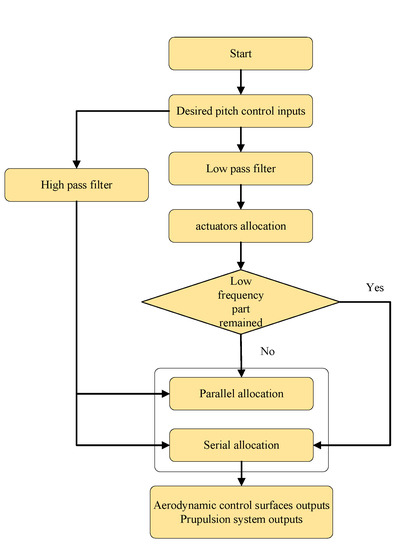
Figure 20.
Control allocation logic.
Take the pitch channel as an example. If the required low-frequency command is less than the maximum elevator efficiency, the low-frequency part is provided by the elevator absolutely, and the high-frequency part is shared by the thrust vector nozzle and elevator parallelly. If the required low-frequency part exceeds the aerodynamic efficiency, the oversized part is compensated by the thrust vector, and the high-frequency part relies on the thrust vector control only.
In Equation (36), and are the elevator deflection angle and the differential speed of the lift fan and thrust vector nozzle, and and are the pitch channel control efficiency of each actuator. and are the aileron deflection angle and differential flow of the side nozzles, and and are their control efficiencies, respectively. and are the rudder deflection angle and thrust vector nozzle deflection angle, whose control efficiencies are and . The control efficiency can be calculated by Equation (37).
Here, is the pitch control derivatives, is the roll control derivatives, and is the yaw control derivatives. is the pitch control efficiency of the propulsion system, which is defined as the differential force of the lift fan and ducted nozzle, and is the length from the center of gravity to the lift-fan fix point. is the roll control efficiency of the side nozzles, which is defined as the roll moment generated by each differential flow unit. , , and are the reference length, area, and span, respectively. , , and are the inertia moments around the body x, y, and z axes, respectively.
Besides the attitude channels, the speed channel also requires an allocator in the transition mode. Due to the peculiarity of the thrust-vector and lift-fan system, the descending rate can be controlled more precisely by the direct lift at a low airspeed, which is also the guaranty of SRVL security.
According to the SRVL deceleration performance analysis, the positive boundary of the forward speed acceleration surpasses the negative boundary significantly. Since the propulsion system only impacts the positive boundary, the control efficiency requirements of the propulsion system are not an issue. This work let the highly efficient propulsion system control the descending rate. The control inputs were . This work let the thrust vector deflection angle, , control the forward speed:
where is the forward flight channel control efficiency, defined as the forward speed acceleration generated by the engine speed unit. is the current trimmed thrust vector deflection angle.
7. The Simulation
In the real-world SRVL, the aerodynamics, flight conditions, and atmosphere environments usually deviate from the nominal conditions, which requires the control system to be robust. Therefore, the robustness performance of the complete SRVL strategy should be verified.
7.1. The Nominal State Simulation
Before testing the algorithms presented in this paper in real flight, more realistic procedures should be implemented to evaluate the performance levels of the algorithms. A hardware-in-the-loop (HIL) simulation was therefore carried out to test and verify in real time the algorithms deployed in the autopilot. The complete HIL architecture is depicted in Figure 21. The architecture comprised two main components, namely, the real-time simulator and the autopilot. The simulator communicated with the autopilot through the full duplex serial link at 400 Hz to receive control instructions, ran the 6-DOF model to calculate the vehicle status (e.g., position, attitude, velocity, etc.), and transmitted sensor data (e.g., inertial measurement unit, GPS, geomagnetism, etc.) to the autopilot. Based on the RC receiver inputs and the sensor information provided by the simulator, the autopilot ran the control program to control the servos and sent back control instructions to the simulator to form a closed loop. In addition, the ground station monitored the flight status in real time. The flight control system was implemented with an approach combining of MATLAB/Simulink and the embedded coder technology to generate the C code for direct deployment. For hardware configuration, the HIL simulation was conducted on the autopilot with a CPU of STM32F765VGT6 216 MHz and the simulator with a CPU of ARM Cortex-A53 1.2 GHz. Furthermore, the controllers ran at 400 Hz with the guidance at 20 Hz.
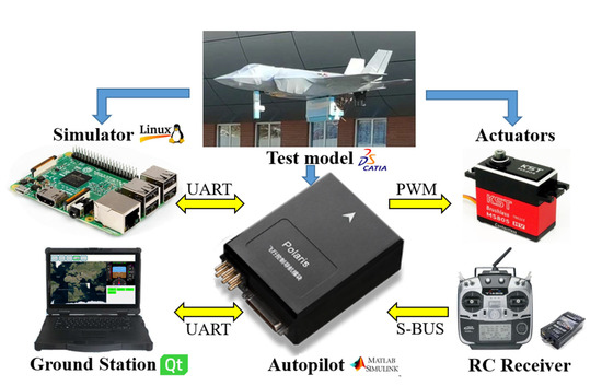
Figure 21.
Hardware-in-the-loop configuration.
First, the nominal state HIL simulation was executed to provide a benchmark and to verify the feasibility of the proposed STOV and SRVL strategy. The takeoff point of the aircraft was set as the origin and it flew along the reference route. The initial mass of the aircraft was 13 kg, and the servo bandwidth was 20 rad/s.
The trajectory simulation results are depicted in Figure 22, with the time history of the flight states depicted in Figure 23.
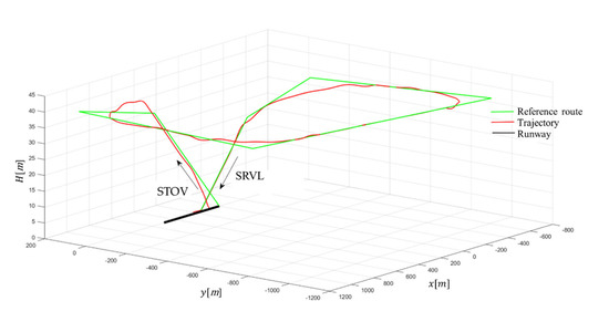
Figure 22.
Nominal flight trajectory.
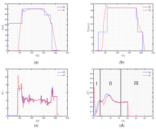
Figure 23.
Time history of the nominal flight states: (a) Altitude; (b) Velocity; (c) Pitch angle; (d) Roll angle.
Figure 22 reveals that the designed control system can provide an excellent trajectory tracking performance in a nominal state and ensure a precise landing at the default landing point. The results depicted in Figure 23 reflect that the aircraft has touched down and enters the ground deceleration stage, which is identical to a normal landing. The touchdown groundspeed was 14 m/s, satisfying the control targets. According to Figure 23, in the whole process simulation, the altitude command tracking deviation of the aircraft was basically kept at about 1 m after stable flight, there was slight vibration near the command, the speed command tracking was accurate, and there was basically no deviation during cruise flight. The deviation of the attitude command tracking was mainly at the end of the takeoff and taxiing section. At this time, the speed of the aircraft reached the ground speed and started to climb. Therefore, the response of the pitch angle had a certain overshoot. After that, the deviation of the pitch angle command tracking in the cruise section was small. There was no deviation in the whole process of rolling angle command tracking.
The nominal state simulation proves that the aircraft’s strategy allows it to short land with the forest flight states and track the control commands.
7.2. The Perturbation Simulation
A Monte-Carlo simulation is a practical method to verify the control robustness performance with the development of contemporary control technologies. It randomly perturbs the model and atmosphere parameters and shoots the state parameters on a massive scale, thus showing the robustness performance directly by the time-domain results. The perturbation parameters are given in Table 5.
Table 5.
Perturbation range of main parameters.
With the random gain imposed on these parameters, the Monte-Carlo results were acquired, as shown in Figure 24.
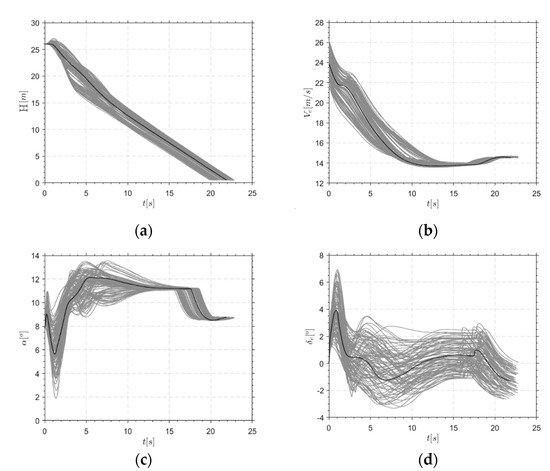
Figure 24.
Monte Carlo simulation results: (a) Altitude; (b) Velocity; (c) Angle of attack; (d) Elevator.
In Figure 24b, the end of the touchdown speed is constrained between 14.18 m/s and 14.69 m/s, which satisfies the requirement that the absolute error should be less than 1 m/s. Figure 24c shows that the angle of attack never exceeded the stall angle of attack of 16°. From Figure 24d, the elevator occupation was less than the limitation of , which means a stability margin still existed in the perturbation states, thus inducing a secure SRVL.
Figure 25a gives the track map of the aircraft, where the three SRVL stages are marked by different colors: red for stage I, yellow for stage II, and blue for stage III. In the perturbed states, there was a deviation of the gliding angle at stage I, it was eliminated significantly at stage II, and at stage III the default gliding angle was achieved and ready for touchdown. Figure 25b presents the landing point distribution results. Explicitly, the landing points were distributed almost in a line inside the a 5 m radius circle centered at the target landing point. This means the proposed strategy is robust enough to reject the lateral displacement due to disturbances and ensure a precise landing.
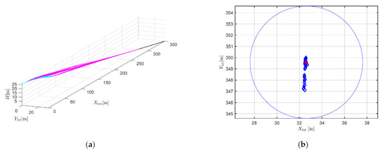
Figure 25.
Aircraft track map: (a) Flight path results; (b) Landing point distribution.
8. Conclusions
This work designed the STO and SRVL strategy for thrust-vectoring V/STOL vehicles based on flying performance and mission requirements that are specified by the AES methods. Then, a NDI-based control structure was applied for the strategy implementation. The hardware-in-loop Monte Carlo simulations provided expected verification results. Thus, the following conclusions are cautiously presented:
- The STO and SRVL strategy should be designed on the basis of specific references. The mission references should consider the specific performance of the aircraft, such as takeoff/landing performance, deceleration performance, speed stability, and trajectory stability. The AES method is a model-based solution for strategy formation.
- The Monte-Carlo simulations verified the robustness performance of the piecewise control structure. The results show that the strategy satisfies the mission requirements and has strong robustness.
- The touchdown state of thrust-vectoring V/STOL can be ensured by the SRVL strategy. The velocity states are decoupled from the overall longitudinal states by entering the stable velocity regions with the attitude states controlled.
Author Contributions
Conceptualization, Z.W. and Z.G.; methodology, Z.G. and Z.W.; software, Z.G. and Z.W.; validation, Z.G., S.M. and T.Z.; formal analysis, Y.C.; investigation, Z.Z.; resources, Z.G.; data curation, Z.W.; writing—original draft preparation, Z.G., S.M. and Z.W.; writing—review and editing, Z.W. and Z.Z; visualization, Y.C.; supervision, Z.G.; project administration, Z.Z. All authors have read and agreed to the published version of the manuscript.
Funding
This research received no external funding.
Institutional Review Board Statement
Not applicable.
Informed Consent Statement
Not applicable.
Data Availability Statement
Data available on request due to restrictions eg privacy or ethical. The data presented in this study are available on request from the corresponding author. The data are not publicly available due to commercial use.
Conflicts of Interest
The authors declare no conflict of interest.
References
- Britt, R.T.; Arthurs, T.D.; Jacobson, S.B. Aeroservoelastic analysis of the B-2 bomber. J. Aircr. 2000, 37, 745–752. [Google Scholar] [CrossRef]
- Jacobson, S.; Britt, R.; Freim, D.; Kelly, P. Residual pitch oscillation (rpo) flight test and analysis on the b-2 bomber. ICES J. Mar. Sci. 2003, 67, 1260–1271. [Google Scholar] [CrossRef]
- Su, W.; Gao, Z.H.; Xia, L. Multiobjective optimization design of aerodynamic configuration constrained by stealth performance. Acta Aerodyn. Sin. 2006, 24, 137–140. [Google Scholar] [CrossRef]
- Ransone, R. An Overview of Experimental VSTOL Aircraft and Their Contributions. AIAA 2002, 64, 1–21. [Google Scholar] [CrossRef]
- Parsons, D.G.; Levin, D.E.; Panteny, D.J.; Wilson, P.N.; Rask, M.R.; Morris, B.L. F-35 STOVL Performance Requirements Verification. In The F-35 Lightning II: From Concept to Cockpit; American Institute of Aeronautics and Astronautics: Reston, VA, USA, 2022; pp. 641–680. [Google Scholar] [CrossRef]
- Goman, M.G.; Khramtsovsky, A.V.; Kolesnikov, E.N. Evaluation of Aircraft Performance and Maneuverability by Computation of Attainable Equilibrium Sets. J. Guid. Control. Dyn. 2008, 31, 329–339. [Google Scholar] [CrossRef]
- Walker, G.; Allen, D. X-35B STOVL Flight Control Law Design and Flying Qualities. In Proceedings of the 2002 Biennial International Powered Lift Conference and Exhibit, Williamsburg, VA, USA, 5–7 November 2002; pp. 1–13. [Google Scholar] [CrossRef]
- Osder, S.; Caldwell, D. Design and robustness issues for highly augmented helicopter controls. J. Guid. Control. Dyn. 1992, 15, 1375–1380. [Google Scholar] [CrossRef]
- Carter, J.; Stoliker, P. Flying quality analysis of a JAS 39 Gripen ministick controller in an F/A-18 aircraft. In Proceedings of the AIAA Guidance, Navigation, and Control Conference and Exhibit, Dever, CO, USA, 14–17 August 2000; pp. 1–20. [Google Scholar] [CrossRef]
- Denham, J. STOVL Integrated Flight and Propulsion Control: Current Successes and Remaining Challenges. In Proceedings of the 2002 Biennial International Powered Lift Conference and Exhibit, Williamsburg, VA, USA, 5–7 November 2002. [Google Scholar] [CrossRef]
- Xili, Y.; Yong, F.; Jihong, Z. Transition Flight Control of Two Vertical/Short Takeoff and Landing Aircraft. J. Guid. Control. Dyn. 2008, 31, 371–385. [Google Scholar] [CrossRef]
- Zian, W.; Shengchen, M.; Zheng, G. Energy Efficiency Enhanced Landing Strategy for Manned eVTOLs Using L1 Adaptive Control. Symmetry 2021, 13, 2125. [Google Scholar] [CrossRef]
- Cao, C.; Hovakimyan, N. Design and Analysis of a Novel L1 Adaptive Controller, Part I: Control Signal and Asymptotic Stability. In Proceedings of the 2006 American Control Conference, Minneapolis, MN, USA, 14–16 June 2006. [Google Scholar] [CrossRef]
- Liu, N.; Cai, Z.; Wang, Y. Fast level-flight to hover mode transition and altitude control in tiltrotor’s landing operation. Chin. J. Aeronaut. 2020, 34, 181–193. [Google Scholar] [CrossRef]
- AIAA. Control configuration design for a mixed vectored thrust ASTOVL aircraft in hover–Navigation and Control Conference (AIAA). Adv. Mater. 2009, 21, 4880–4910. [Google Scholar] [CrossRef]
- Yang, Z.F.; Lei, H.M.; Li, Q.L.; Li, J. A missile control system design approach based on dynamic inverse and robust trajectory tracking control. Yuhang Xuebao/J. Astronaut. 2011, 32, 317–322. [Google Scholar]
- Toha, S.F.; Tokhi, M.O. Dynamic Nonlinear Inverse-Model Based Control of a Twin Rotor System Using Adaptive Neuro-fuzzy Inference System. In Proceedings of the Third Uksim European Symposium on Computer Modeling & Simulation IEEE Computer Society, Athens, Greece, 25–27 November 2009. [Google Scholar] [CrossRef]
- Fan, Z.Q.; Fang, Z.P. Robust, nonlinear control design for a post-stall maneuver aircraft. Acta Aeronaut. Et Astronaut. Sin. 2002, 23, 193–196. [Google Scholar] [CrossRef]
- Bodson, M. Evaluation of optimization methods for control allocation. J. Guid. Control. Dyn. 2002, 25, 703–711. [Google Scholar] [CrossRef]
- Burken, J.; Lu, P.; Wu, Z.; Bahm, C. Two reconfigurable flight-control design methods: Robust servomechanism and control allocation. J. Guid. Control. Dyn. 2012, 24, 482–493. [Google Scholar] [CrossRef]
- Falkena, W.; Borst, C.; Chu, Q.P.; Mulder, J.A. Investigation of Practical Flight Envelope Protection Systems for Small Aircraft. AIAA Guid. Navig. Control. Conf. 2011, 34, 976–988. [Google Scholar] [CrossRef]
- Yu, Z.; Li, Y.; Zhang, Z.; Xu, W.; Dong, Z. Online safe flight envelope protection for icing aircraft based on reachability analysis. Int. J. Aeronaut. Space Sci. 2020, 21, 1174–1184. [Google Scholar] [CrossRef]
- Lombaerts, T.; Schuet, S.; Acosta, D.; Kaneshige, J.; Shish, K.; Martin, L. Piloted simulator evaluation of safe flight envelope display indicators for loss of control avoidance. J. Guid. Control. Dyn. 2016, 40, 948–963. [Google Scholar] [CrossRef]
- Cheng, Z.; Zhu, J.; Yuan, X. Design of optimal trajectory transition controller for thrust-vectored V/STOL aircraft. Sci. China Inf. Sci. 2021, 64, 139201. [Google Scholar] [CrossRef]
- Aguiar, A.P.; Hespanha, J.P. Trajectory-tracking and path-following of underactuated autonomous vehicles with parametric modeling uncertainty. IEEE Trans. Autom. Control. 2007, 52, 1362–1379. [Google Scholar] [CrossRef]
- Chunzhe, Z.; Yi, H. ADRC Based Integrated Guidance and Control Scheme for the Interception of Maneuvering Targets with Desired LOS Angle. In Proceedings of the 29th China Control Conference, Beijing, China, 29 July 2010; ISBN 978-7-8946-3104-6. [Google Scholar]
- Shakarian, A. Application of Monte-Carlo Techniques to the 757/767 Autoland Dispersion Analysis by Simulation. Guid. Control. Conf. 1983, 83, 181–194. [Google Scholar] [CrossRef]
- Williams, P. A Monte Carlo dispersion analysis of the X-33 simulation software. In Proceedings of the AIAA Atmospheric Flight Mechanics Conference and Exhibit, Montreal, QC, Canada, 6–9 August 2001. [Google Scholar] [CrossRef]
- Chao, Z.; Lei, C.; Zongji, C. Monte Carlo Simulation for Vision-based Autonomous Landing of Unmanned Combat Aerial Vehicles. J. Syst. Simul. 2010, 22, 2235–2240. [Google Scholar] [CrossRef]
- The Pla General Armament Department. Gjb 3719-99; Ship-Based Airplane Specification (Flying Qualities) [S]; The PLA General Armament Department: Beijing, China, 1999; pp. 16–19. [Google Scholar]
- Ding, Y. Study on Ducted Vertical Take-Off and Landing Fixed-Wing UAV Dynamics Modeling and Transition Corridor. Appl. Sci. 2021, 11, 10422. [Google Scholar] [CrossRef]


Publisher’s Note: MDPI stays neutral with regard to jurisdictional claims in published maps and institutional affiliations. |
© 2022 by the authors. Licensee MDPI, Basel, Switzerland. This article is an open access article distributed under the terms and conditions of the Creative Commons Attribution (CC BY) license (https://creativecommons.org/licenses/by/4.0/).