Abstract
Especially for electric vehicles, the tire impact on car noise is becoming more and more important. The requirement of meeting certification criteria makes estimating the sound pressure level essential for vehicle manufacturers. Most recent research on tire road noise is conducted on component test benches. Little research exists into tires mounted on vehicles, and even less into the impact of acceleration on the generated noise. The literature mainly considers some vehicle shape differences, tire load, and inflation pressure. This article investigates the impact of different vehicles on tire noise through a series of measurements on a standardized test track. The rolling noise as well as accelerated noise of three different tires and five different vehicles are compared. The impact of the drive axle on accelerated noise as well as a weight variation is investigated. Additionally to the absolute measured differences between the vehicles, statistical methods are used to separate measurement dispersion from actual systematic differences. This research therefore validates older research on the vehicles’ impact on tire noise, which is necessary since the general tire structure, thread, and rubber composition have changed in the time period between the publication of previous research from the literature and this paper. This allows us to approximate the emitted noise on different vehicles. Furthermore, we validate an algorithm to virtually change tires on test benches. The algorithm is standardized and implemented in common measurement software.
Keywords:
tire noise; pass-by; rolling noise; accelerated noise; vehicle certification; NVH; regression 1. Introduction
Although vehicle noise, especially engine noise, might be linked to positive emotions for the driver, the average pedestrian will consider loud vehicles disturbing. The sound pressure level (SPL) experienced by pedestrians is important since even low SPLs might cause health issues like, e.g., sleep disturbance if the exposure is long enough [1]. Due to this, the overall emitted SPL of vehicles is regulated by governmental institutions, making it necessary for vehicle manufacturers to ensure that they meet the regulation [2].
Tire noise has a dominant role in the certification of exterior noise. This strong impact was already in place for classic vehicles with an internal combustion engine (ICE) [3] and becomes even stronger for electric vehicles (EVs) [4,5].
It is, therefore, important to ensure that the impact of the tire noise on the overall noise is recorded accurately. Assuming that the interaction between vehicles and tires does not differ strongly for different tire vehicle combinations, e.g., power levels of the engine, a virtual tire changing algorithm is implemented in common measurement software (i.e., Pak Pass-By (Software by Müller-BBM VibroAkustik Systeme GmbH)). This algorithm basically takes tire noise measurements that are conducted on vehicles that did not emit noise other than tire noise, and transforms these on regular measurements. In addition, the tire changing algorithm enables the simulated pass-by noise measurement of the whole vehicle. These are conducted on a roller test bench. Since the interaction between the reel and treaded tire is not comparable with the interaction between the street and treaded tire, a method to convert measurements from test bench to road measurements is necessary. The changing algorithm therefore separates the overall external tire road noise into rolling and accelerated parts. In this research, the rolling noise is referred to as the external noise produced by the tire with the vehicle in idle mode. The accelerated noise is the delta of the SPL during accelerated runs compared to runs in idle mode. The tire noise is the sum of both parts.
The rolling noise can be described as a logarithmic function over the driving speed ([6] p. 172), while the accelerated noise is described as a polynomial of second degree over the acceleration [7]. To calculate both functions, regression coefficients must be determined. This is done through a series of freely rolling measurements, e.g., runs with constant speed and accelerated measurements. The used vehicle must be one with ICE whose external sound is completely isolated, or an EV. The regression coefficients are calculated on every point of the test track. They are used together with the driving dynamics to calculate an SPL for each point of the test track. By subtracting one tire’s SPL curve from the overall measured SPL curve of a measuremnt with ICE vehicle and adding another tire’s SPL curve, a virtual tire change is performed.
Even though this procedure is implemented as standard, the authors could not find any research on the accuracy of the process. To gain more insight, a measurement series is conducted which takes a deeper look at the vehicle impact on the tire noise. The vehicle’s impact is especially important for the changing algorithm since it thereby made use of the assumption that the emitted tire noise is independent of the vehicle. While looking at the results of the measurement series, the variance in the regression coefficients is also analysed to generate knowledge on the dispersion of the SPL curves and thus the maximum possible accuracy of the process.
Less recent research conducted by Ejsmont and Sandberg [8] specifically investigated the vehicle’s impact on tire noise. Thereby, only rolling noise was a topic of the research. The authors carried out coast-by runs at the speed of 30 to 90 in steps of 20 . 8 different vehicles, subdivided in heavy and light cars, four each, were measured with the same tire for all vehicles in one category. The smallest difference between vehicles in one category was recorded at 70 with a maximum difference of dB(A). [8]
The Tire/road noise: Reference book by Sandberg and Ejsmont [6] gives a general overview of research regarding tire road noise before 2002. Thereby, a highly investigated impact on tire road noise is the tire load. The presented research comes to the conclusion, that higher load leads to higher SPL. The authors cite a Ph.D. thesis written by Taryma Stansilaw (Thesis from Taryma Stansilaw from 1982, due to original language not available to author) stating that, without adaption of the tire inflation pressure, a doubling in load leads to an increase of to dB(A), if the pressure level is adapted an increase of 1 to 2 dB(A) is recorded [6].
The impact of wheel housing was also investigated by Ejsmont et al. [9]. A difference of dB(A) from the same tires mounted on different vehicles in the near field of measurements conducted on a drum was reported. Adding sound absorbing material in the wheel house to reduce overall SPL was also tested but did not lead to any noticeable difference. The authors assumed that during pass-by measurements at a microphone distance of the difference due to wheel housing design is lower than the measured differences in close-proximity of the tire [9].
More recent research by Stalter et al. [10] investigated the impact of driving torque on accelerated noise in the near field on a test bench with a safety-walk. The measurements indicated an additional SPL of 4dB at approximately 1020 . The authors also investigated different profile structures and came to the result that the impact in the case of tires with soft circumferential stiffness is rather low compared to the impact on those with harder circumferential stiffness [10].
The authors Grollius and Gauterin [11] conducted similar near field measurements on a test bench with different tires, including two summer tires, a slick, and two experimental thread patterns. The authors subdivided the results in two frequency ranges 1250 to 1550 and 2500 to 3400 since in these ranges the measured data seemed not influenced by noise of the driving engine. Averaging the results of the two summer tires, a difference between rolling noise and accelerated noise at 2500 peripheral force of and for the first and second frequency range was reported. Nevertheless, neither research proposal investigated the acceleration impact at microphones situated at pass-by positions. [11].
Some recent research on the impact of acceleration in SPL is presented in Hoever et al. [12]. The authors found a rather strong correlation between two different vehicles with the same tires mounted for constant driving conditions and a rather weak correlation for accelerated measurements [12]. In their corresponding presentation slides [13], they show additional tires and their accelerated behavior. Thereby, it is notable that the average mathematical model found to explain the additive SPL of acceleration only reaches a coefficient of determination (COD) of 0.44, with max value of 0.9 and min value of 0.1.
The legal limits for the external noise of vehicles are getting smaller and smaller, especially in the case of EVs for which only the tire has an influence. Due to this, it is essential for vehicle manufacturers to know which differences can be expected due to different vehicles. The purpose of this research is therefore divided into two main aspects. Firstly, the overall vehicle impact on exterior tire noise rolling and accelerated is investigated. This is also necessary to validate the tire changing algorithm. Even though the vehicle impact was already investigated in literature, since these were conducted, tire construction and materials changed heavily. This raises the question whether the same difference will be obtained with modern tires. Secondly, the impact of the drive axle on accelerated noise behaviour as well as overall difference resulting from acceleration in the far field of the tires is investigated.
Other than the impact of the vehicle and the acceleration, the road surface and texture as well as tire texture have a large impact on the overall tire noise. Nevertheless, these issues are not in the scope of the provided research. Some relevant literature on these topics can be found in [6,14,15,16,17,18].
First, the experiment design is shown. Afterwards we explain how measurements are conducted and digitally processed. Thereby, different regression methods are also investigated. These topics are followed by the measurement results. The results are subdivided into five subsections: one for each of the tires investigated, one for a temperature impact investigation, and one for an error evaluation of the recorded data. Then, the tire changing algorithm is explained and validated. The last chapter summarizes all interim conclusions and provides an outlook of research to come.
2. Experiment Design
Following the design of experiments (DoE) as well as the reasoning for the construction of the DoE is explained. In total, three different tires are investigated, on five different vehicles. Each used vehicle is either a Hybrid Electric Vehicle (HEV) or a Battery Electric Vehicle (BEV) Figure 1 and Figure 2 show the full DoE with each arrow indicating one measurement series.

Figure 1.
First block of experiments.
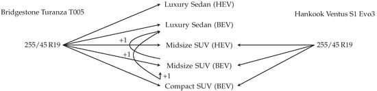
Figure 2.
Second block of experiments, +1 indicating an additional weight adaption of the vehicle.
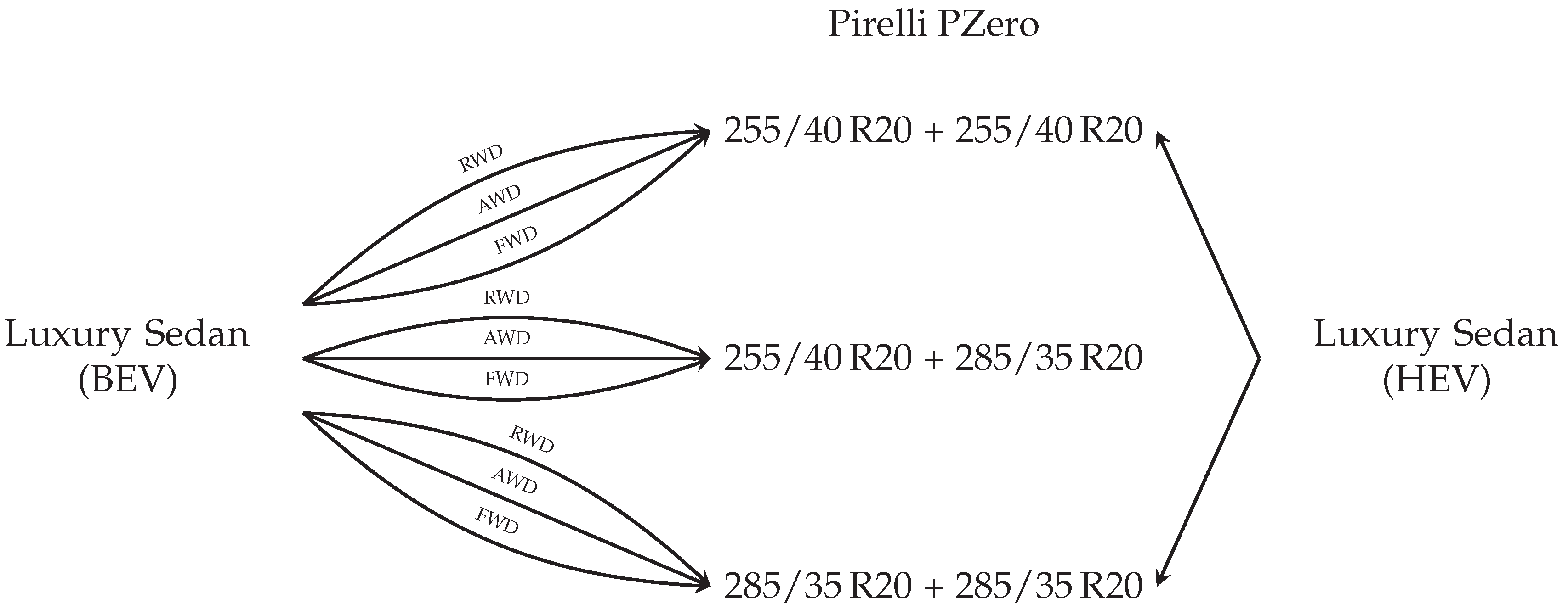
The DoE is separated into two larger blocks. The focus on the first block is to investigate the impact of the drive axle on the accelerated tire noise. Thereby, all wheel drive (AWD), front wheel drive (FWD) and rear wheel drive (RWD) are investigated. The variation in drive axle is possible since the used EV has different electric machines for each axle. With according software tools, these can be switched off allowing the three different drive modes. To further validate the virtual tire change, a hybrid car is also used for measurements. The tire notation, shown in the center of Figure 1, describes the mounted ones on front axle + rear axle.
The second block, as shown in Figure 2, addresses the overall impact on rolling noise as well as accelerated noise of different vehicles. Therefore, five different vehicles, including three electric and two hybrid ones are used for the measurements. Each arrow indicates one measurement series with the tire, the arrow starts from, mounted on the vehicle, the arrow points at. Arrows notated with a + 1, visualize an additional weight adaption. The tire mounted in these cases is the Bridgestone tire.
In total the design of experiment includes 22 measurement series.
To make the following paragraphs more readable, the tires are only referred to through their width and the first letter of the manufacturer. Leading to, e.g., 255P for . In case of mixed mounted tires, they are referred to as front axis + rear axis. A translation tabular is available in Table A1. The used vehicles are furthermore referred to as the first letter of the vehicle categories, first letter of the shape, and the corresponding abbreviation of the powertrain (e.g., MSHEV for Midsize SUV HEV). An alternative presentation of the DoE can be found in the Table A2 and Table A3.
The Pirelli PZero is available in different dimensions. In the following measurements, two different tire widths 255/40 R20 and 285/35 R20 are used. They are mounted on rims with identical design, that only differ in their width. In the case of the wider 285P wheels mounted on the front axes, distance plates with a thickness of 20 had to be inserted between the rim and wheel bearing.
3. Measurement Procedure
The measurements are carried out on the noise track of the Applus+ IDIADA company in Spain. This decision was made in order to keep environmental variations, especially temperature changes minimal.
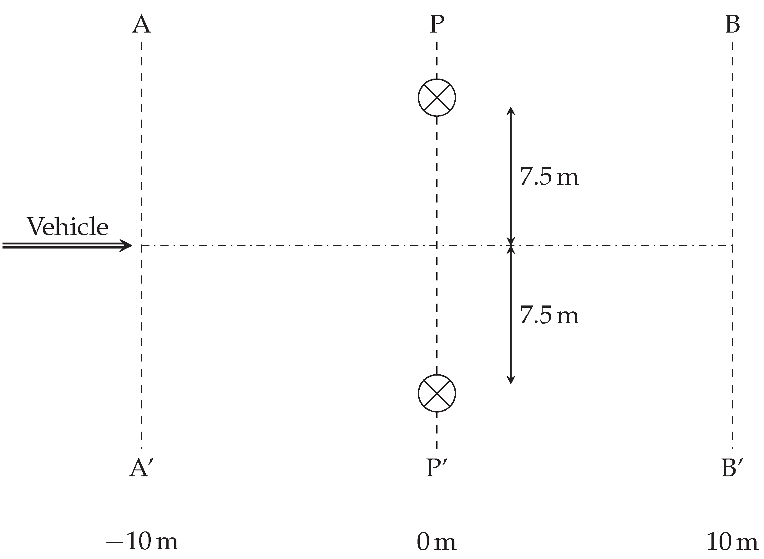
The measurements track is constructed equivalent to the one described in UN/ECE Regulation No. 117 [19]. Figure 3 shows the different points of the test track. The test track includes two microphones at a height of , one on each side of the track, at a distance of to the center line at the 0 location of the track.
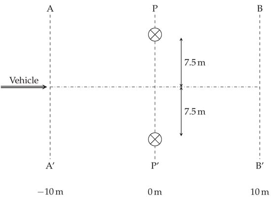
Figure 3.
Principal sketch measurement track.
For each tire car combination, rolling noise is measured by driving through the test track with speeds between 40 and 90 . Thereby, the speed is increased in steps of 5 leading to a total of 22 idle measurement since every speed is repeated to minimize measurement errors.
Furthermore, accelerated runs are recorded. Thereby, the speed at P-P’ is set to be 50 . The car is accelerated at least entering A-A’. The average acceleration between A-A’ and B-B’ is automatically calculated by the used measurement software (PAK Pass-By 3.2 from Müller-BBM VibroAkustik Systeme GmbH). Considering the average track acceleration, five steps between and are recorded. This acceleration differs from instantanous acceleration at P-P’, which is why further shown figures also show greater accelerations. In the case of hybrid cars (LSHEV and MSHEV), only three acceleration steps are recorded. The acceleration steps are realised through changing the fixed gear and driving full throttle (ICE) and through attaching small spacers to the gas pedal, to limit the maximal gas pedal position (EV). Each acceleration step is repeated four times.
For each run, data is recorded at steps of 0.2 m. A data point consists of speed, distance, elapsed time, SPL at both microphones, air temperature, road temperature, wind speed, wind direction, air pressure, and humidity.
4. Measurement Processing
To ensure comparability and minimize variations, all data points recorded are filtered by the following rules:
- wind speed < 5
- speed at P-P’ of target speed
- SPL left - SPL right ≤ 1 dB(A)
To generate curves for the rolling noise, the original least square method is applied. For the acceleration noise, a weighted constrained regression is applied. The weighting of points is used to decrease the impact of data points clustered at the same x-axis section. This is necessary because only the average acceleration between the entry and exit point of the test track is given when performing the measurements. That acceleration is often slightly different from the local acceleration at the centerline of the track. Therefore, weighting the data points differently is reasonable. All speed measurements are smoothed with a Savgol filter [20] before being used for acceleration calculation. The filter window is thereby set to 11 data points, so that every point is smoothed with data from before and after one meter. The order of polynomial used for fitting is set to one. Following, the mathematical methods used for regression are described. In addition, a method to estimate a density probability of a data set is explained. Thereby, matrices are marked as bold capital letters, vectors as bold lower case letters and estimated values are marked through a hat.
4.1. Least Square
The rolling noise of tires is often recorded to be a logarithmic equation with dependency of the vehicles speed [6]. The A-weighted [21] SPL can therefore be described as
with a and b as constant parameters and v as vehicle speed in .
Equation (1) can be interpreted as a system of linear equations, where each equation describes one run, as shown in (3). If the equation system is over determined, multiple possible solutions can be found. For this reason, the norm of recorded data vector and data vector calculated with a best guess of parameters and is defined. The following minimization problem is referred to as the least square problem. The vector in brackets is referred to as residual
is the vector of regression coefficients, X is the input data set and y is the output data set.
To apply the least square problem on the specific equation system, the data needs to be restructured as follows
It is possible to solve the problem analytically, leading to the following term.
4.2. Weighted Least Square
For datasets with data that is not uniformly distributed over the range of possible input ranges, or heteroscedastic datasets, the weighted multiple linear regression is more suitable.
The weight matrix can arbitarily weight each data point individually or even eliminate their impact on the regression completely. Even though the weight matrix might be manually constructed, different approaches of how to generate these automatically and the impact of the weight functions on the regression were studied in Ruppert and Wand [22].
4.3. Constrained Least Square
Another method of manipulating the regression is to constrain the least square problem. This allows us to implement previous knowledge in the resulting regression model. In case of the accelerated tire noise, this is very useful. The authors of ISO 362-3:2016 [7] define a function for the accelerated (acc) tire noise as polynomial of second degree [7]
Nevertheless, a large value for the parameter e does not seem physically plausible since it would lead to a large variation in the absolute SPL as result of minimal acceleration. For this reason, the parameter is constrained as dB(A) [7].
The problem definition explained in (2) is supplemented with a constraining objective
where each row of C defines one restriction of the according value d. Boyd and Vandenberghe [23] explain in depth how to solve a constrained least square problem via different methods, e.g., QR factorization and KKT equations. These algorithms are suitable for linear constrained regression systems [23].
4.4. Kernel Estimation and Weighting Function
Even though the weight matrix described in Section 4.2 might be constructed by hand, this is not a practical approach. Weight matrices can be calculated fully automated using the kernel estimation approach.
The key idea behind the kernel estimation is to guess the probability density function of a data set by adding density kernels of each data point to a global distribution. A full explanation of how to calculate these kernel density functions can be found in Chen [24].
The received distribution can be used to generate local weights for each data point. The authors of Steininger et al. [25] provide a method to calculate these weights according to the density of the output data set [25]. Nevertheless, the provided function can be applied on the input data as well, making it possible to evenly distribute the impact of areas with more data points than others on the regression coefficients.
An analysis of different kernel functions and their impact on the global density function can be found in Węglarczyk [26]. It thereby seems that the chosen kernel function is less important than the bandwidth, which in essence defines the width of a kernel [26].
In this research, a gaussian kernel with bandwidth of as kernel function is applied. The weights for each data point are calculated as follows.
with and p as value of the kernel density distribution for the specific acceleration. These values ensure that no point is weighted with a lower importance than 50%.
The accelerated regression curves are obtained via an Levenberg-Marquardt based an optimizer of the [27] python library. The constraint dB(A) leads to a non-linearity in the equation system. This system is not solvable as closed form so that an optimizer is used.
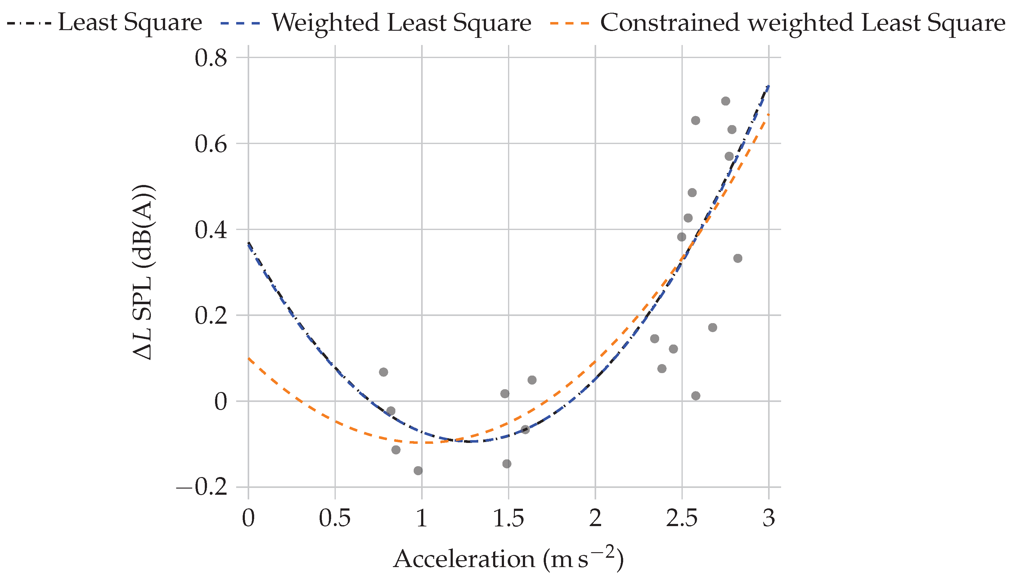
Figure 4 shows the impact of the three different regression algorithms on the calculated curves on the measurement conducted with LSBEV in front drive mode and 255P. It is visible that the sole weighting of single data points does not impact the result for the displaced measurement. This is not surprising since the data points in this run are evenly distributed over the x-axis. Nevertheless, a constrained least square leads to different results in the lower acceleration range. This is physically more plausible than the other curves, which is why that algorithm is used further in this research to calculate the regression coefficients for accelerated noise.
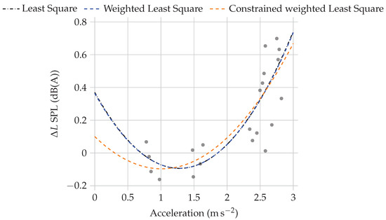
Figure 4.
Impact of different regression algorithms for the measurement of 255P mounted on LSBEV driven with FWD and MB-Correction (Section 5.1) applied.
5. Results
In this section, the results of the processed measurements are presented. They are subdivided into five subsections: one regarding the temperature impact on tire noise, one regarding a general error evaluation and one for each of the tire brands.
In the case of rolling noise, a simple least square problem is solved. On the accelerated dataset, a constrained least square approach, as explained in Section 4, is applied. The output value of the accelerated regression is calculated according to ISO 362-3:2016 [7] as
is an accelerated measurement, is the SPL calculated with (1) and is the delta in SPL between the former two.
All plots shown in the following sections show the measurement results received at the moment the vehicle passes point P-P’. The point marks the center of the test track and therefore the point with the smallest distance between microphones and vehicle.
5.1. Temperature Correction
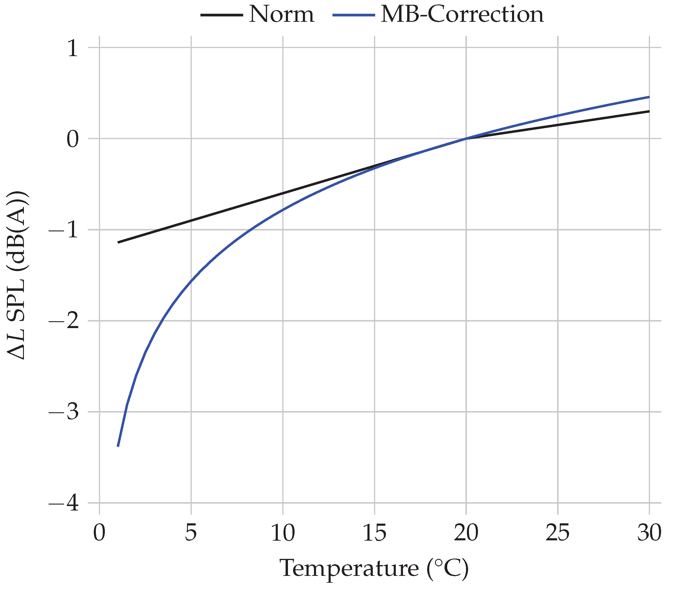
To evaluate the measurement and to make measurements with different environmental conditions comparable, two temperature corrections are compared. The correction curves, as shown in Figure 5, are similar in the area of 10 to 30 but differ greatly below that range.

Figure 5.
Two different temperature correction curves for absolute SPL, reference temperature is 20 °C.
The curve labelled as Norm is the one that is usually applied on standardized measurements according to UN/ECE Regulation No. 51 [2] and UN/ECE Regulation No. 117 [19]. The alternative curve is one that was constructed out of the experience that measurement engineers at Mercedes-Benz gained; therefore, it is referred to as MB-Correction.
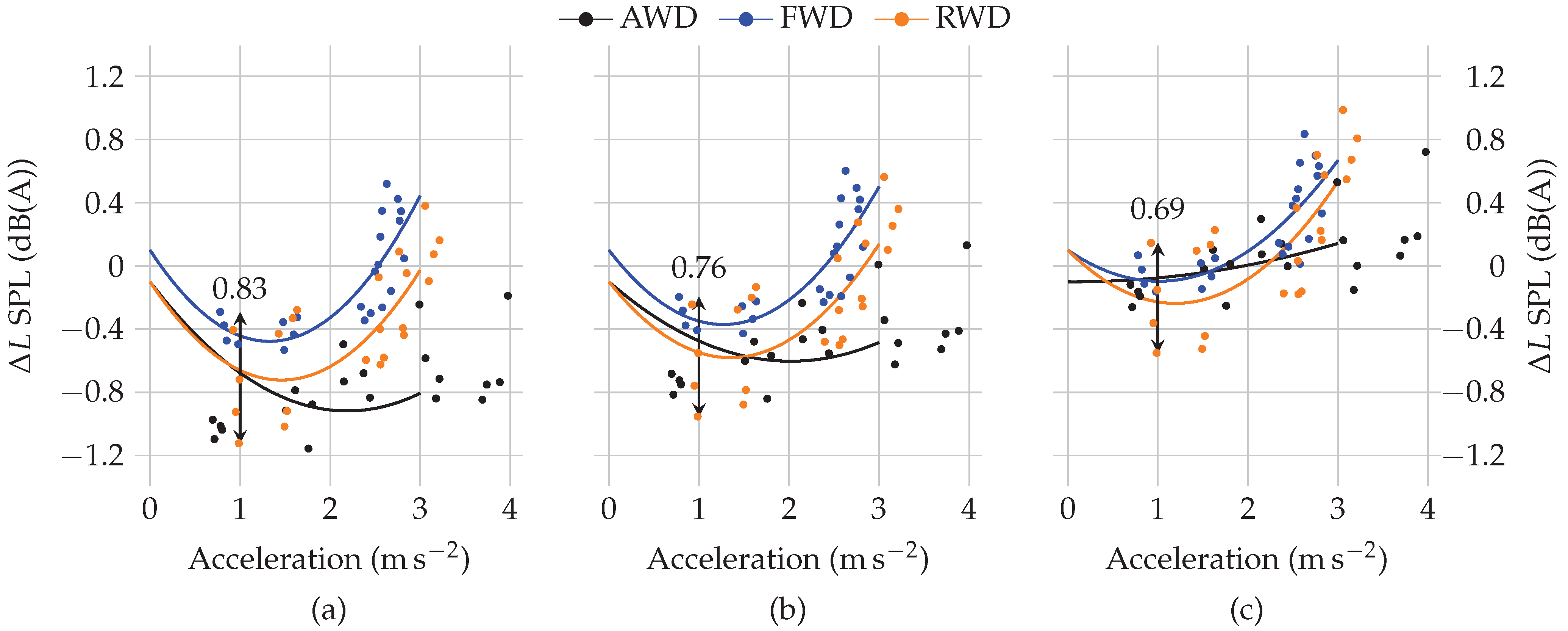
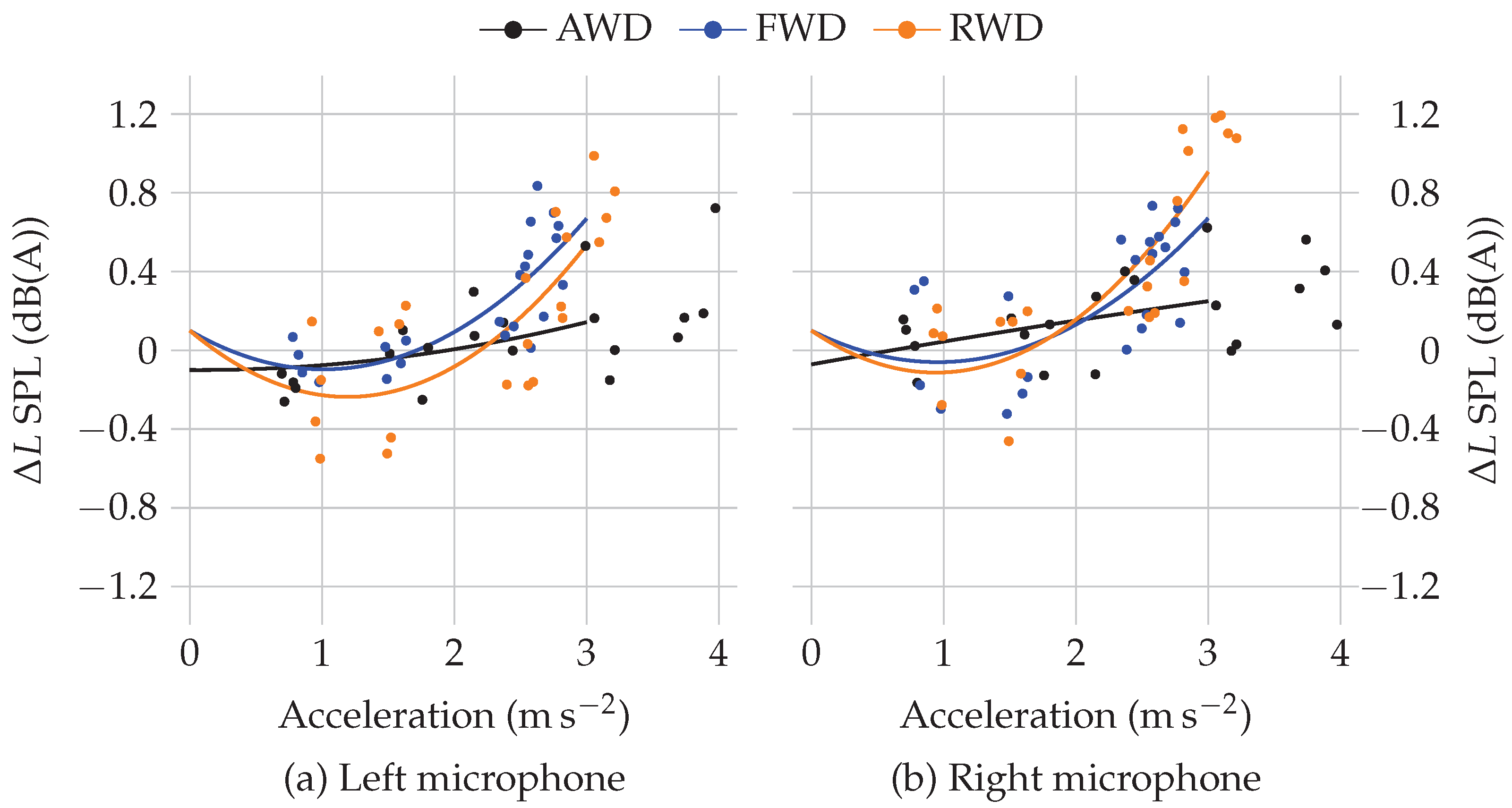
To analyze the impact of the temperature correction on measurements, the accelerated runs for 255P mounted on LSBEV are presented in Figure 6. Figure 6a shows the original recorded data, Figure 6b the norm corrected data and Figure 6c the MB-Correction corrected data. To apply the corrections, the air temperature is used. Each point indicates one accelerated run. The rolling coefficients are calculated once for tire 255P and through Equations (1) and (9) the accelerated noise is calculated. Since the rolling and accelerated measurements are conducted one after another, the air temperature changed from rolling at , to AWD at to RWD at to FWD at , making them viable to investigate the impact of temperature correction.
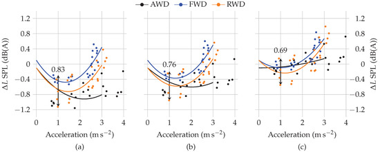
Figure 6.
Impact of different temperature corrections on acceleration induced tire noise of one tire at point P-P’ on the left microphone. (a) Original 255P on LSBEV; (b) Norm Correction 255P on LSBEV; (c) MB-Correction 255P on LSBEV.
Under constant environmental conditions, the three curves are assumed to reach a delta of 0 dB(A) at an acceleration of 0 . The constant offset is therefore mostly explained through the impact of the temperature since no data is processed for runs with higher wind speed than 5 , which means no impact from wind needs to be assumed.
Applying the norm temperature correction as well as the MB-Correction curve on the data set leads to different results. The MB-Correction leads to the lowest difference of all data points in the lower acceleration areas, as indicated by the arrows with corresponding values of dB(A), dB(A), and dB(A). In theory, for an acceleration of 0 , the data points should coincide. This is due to the assumption that no acceleration is almost equivalent to idle runs, and for idle runs no impact of the drive axle is assumed. Because of the observation, that the data point best coincides in the low acceleration range with MB-Correction. From this point in the paper, this correction is applied to all presented data.
5.2. Pirelli PZero
The impact of drive axle on the accelerated noise in addition to the impact of two different vehicles and the difference between mixed mounted and identical mounted tires is presented.
5.2.1. Rolling Noise—Mixed Mounted Impact
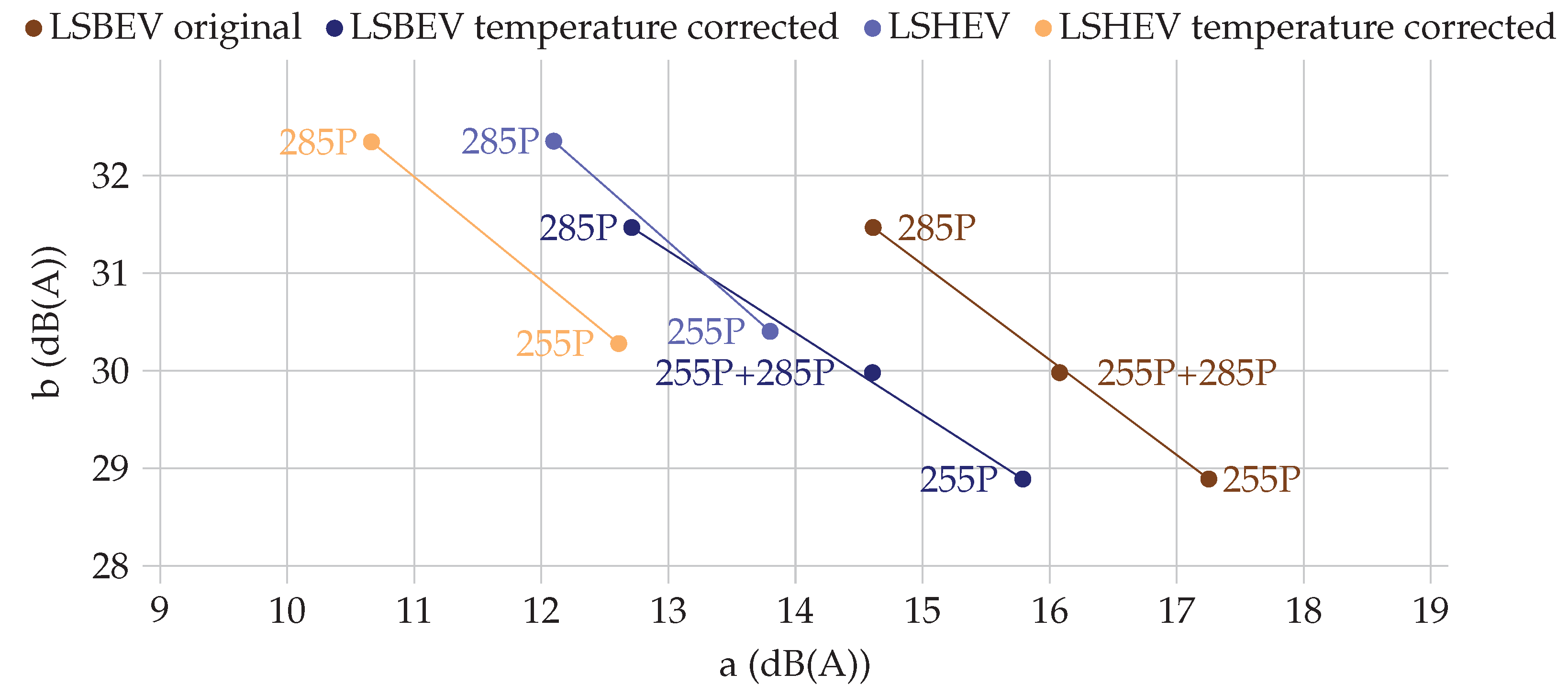
Figure 7 shows the regression coefficient of the rolling noise, received for mixed and identical tires with and without MB-Correction for air temperature. Measurements are conducted with the LSBEV and LSHEV
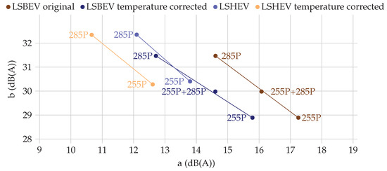
Figure 7.
Impact of mixed mounted tires on rolling coefficients used in (1).
The results show that the combination of 255P+285P lies almost on a linear connection between the 255P and 285P measurements. This indicates that there is almost no interaction between the sound profiles of the different tires but solely a linear overlapping. The load per axle, measured without driver only varies by 24 , with front axle being less loaded. Nevertheless, adding the driver as well as a slight negative acceleration due to air and rolling resistance, which both add more dynamic load on the front axle than the rear axle, the front axle is assumed to carry a higher dynamic load than the rear axle.
Looking at the relationship of identical tires mounted on different cars, a clear trend is visible. The relation between tire 255P and tire 285P mounted on different cars, as indicated by the slope of the connecting lines, does not change as much as the absolute values of each tire on different vehicles. This shows a dependency of the rolling noise of the used vehicle, and leads to the assumption that the vehicle design criteria has a fixed impact on every mountable tire. In numbers, the SPL of the LSBEV driving 50 is dB(A) and dB(A) louder than on the LSHEV for the tires 255P and 285P. The average temperatures of the measurements are shown in Table 1. Taking into account that the temperature correction may have an error as well, it is reasonable to assume that the correction leads to a slight underestimation of the 285P mounted on the LSBEV, which would lead to a near constant error between LSHEV and LSBEV of dB(A). That hypothesis is being supported by the figure as well, since it shows that the temperature correction almost solely affects the a coefficient (as can be seen by the pure shift to the left in the figure).

Table 1.
Air temperature of Pirelli PZero rolling measurements.
5.2.2. Accelerated Noise-Impact of Drive Axle and Mixed Mounted Tires
As shown in Equation (9) the impact of acceleration on tire noise can be extracted trough subtracting the rolling noise from an accelerated measurement that is achieved with an acoustic isolated vehicle or an EV.
Since the drive axle of a vehicle does not impact the rolling coefficients, in the following presented measurement series, coefficients a and b are once calculated and only the accelerated measurements are repeated with different drive axle settings. This leads to a difference in the temperatures between the accelerated runs and the idle runs. The idle runs used to calculate are therefore temperature corrected before the calculation of .
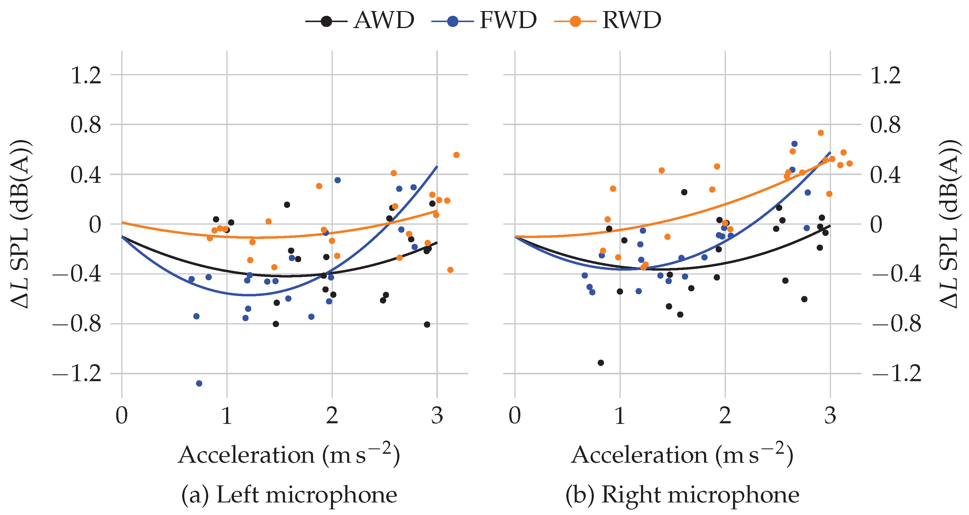
Figure 8 shows the air temperature corrected data for the 255P measured on LSBEV in three different drive modes.
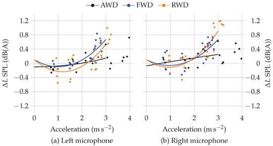
Figure 8.
Air temperature corrected additional SPL caused through acceleration for the 255P mounted on the LSBEV for left and right microphone side on Point P-P’ of the measurement distance.
The presented measurement support the thesis of Stalter [28] that in general high torque leads to higher SPLs [28].
Since the acceleration, shown on the x-axis, indicates the instantaneous acceleration of the vehicle, it does not directly indicate the torque or slip on each tire. Nevertheless, it is assumed that the total torque of all driven wheels is constant, leading to much higher torques on each wheel if there is only one drive axle. This is seen in the comparison between two wheel drive and AWD. The former results in higher torque and therefore slip on the powered tires, which is why the slope is greater than for the four wheel drive.
As shown in Figure 9, in the case of the 285P the trend is not clearly visible. Still, with temperature correction applied, the slope of the curves for single drive axle setting seem to be higher in the range from to than in the case of AWD. The regression curves reach, with an average COD of , lower COD as in the case of the 255P and an average of . It seems rather astonishing that the investigated 255P as well as the 285P emit less sound when slowly accelerating than rolling.

Figure 9.
Air temperature corrected additional SPL caused through acceleration for the 285P mounted on the LSBEV for left and right microphone side on Point P-P’ of the measurement distance.
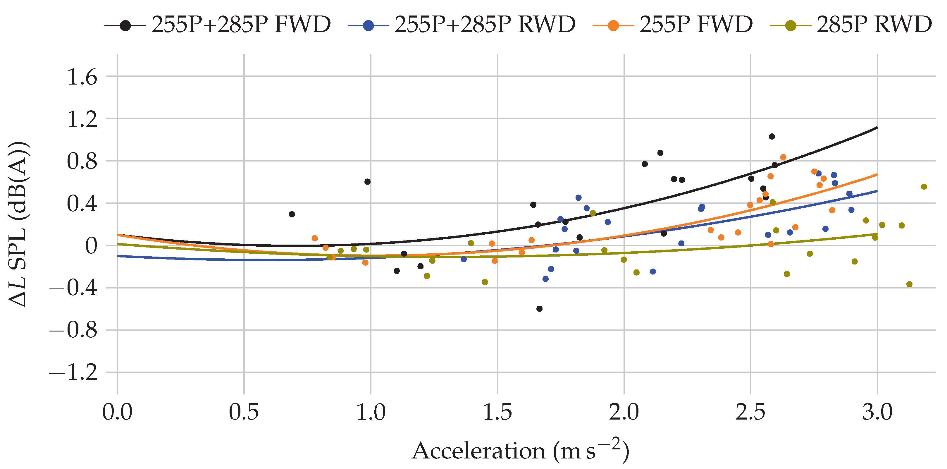
Since the three drive axle variations are measured for three tire combinations with an EV, it is also possible to investigate whether the accelerated coefficients are also impacted by the tire that is not under torque. Therefore a comparison between the scenarios 255P with FWD, 255P + 285P with FWD, 285P with RWD and 255P + 285P with RWD is shown in Figure 10.
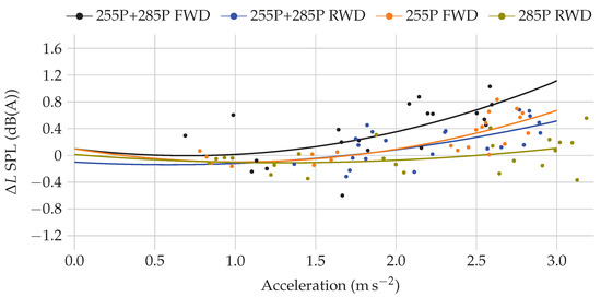
Figure 10.
Air temperature corrected additional SPL caused through acceleration compared between drive axle variation for mixed and identical mounted tire combinations for left microphone side on Point P-P’.
It is visible that the regression lines for the 255P under torque have a higher slope than the curves for the 285P under torque. This seems reasonable since previous figures showed that putting the narrower tire under torque also lead to a much steeper curve than for the wider tire. Nevertheless, the effects do not seem to be completely separable. No two curves happen to have the same slopes. It seems that the tire that is not under torque still has a rather large impact on the accelerated noise behavior of the vehicle. This is indicated by the fact that the tire not under torque still changes the slope of the regression curve. Nevertheless, the impact of the tires under torque seems to be stronger on the overall behavior, which also would be the rather obvious assumption.
5.3. Hankook Ventus S1 Evo3
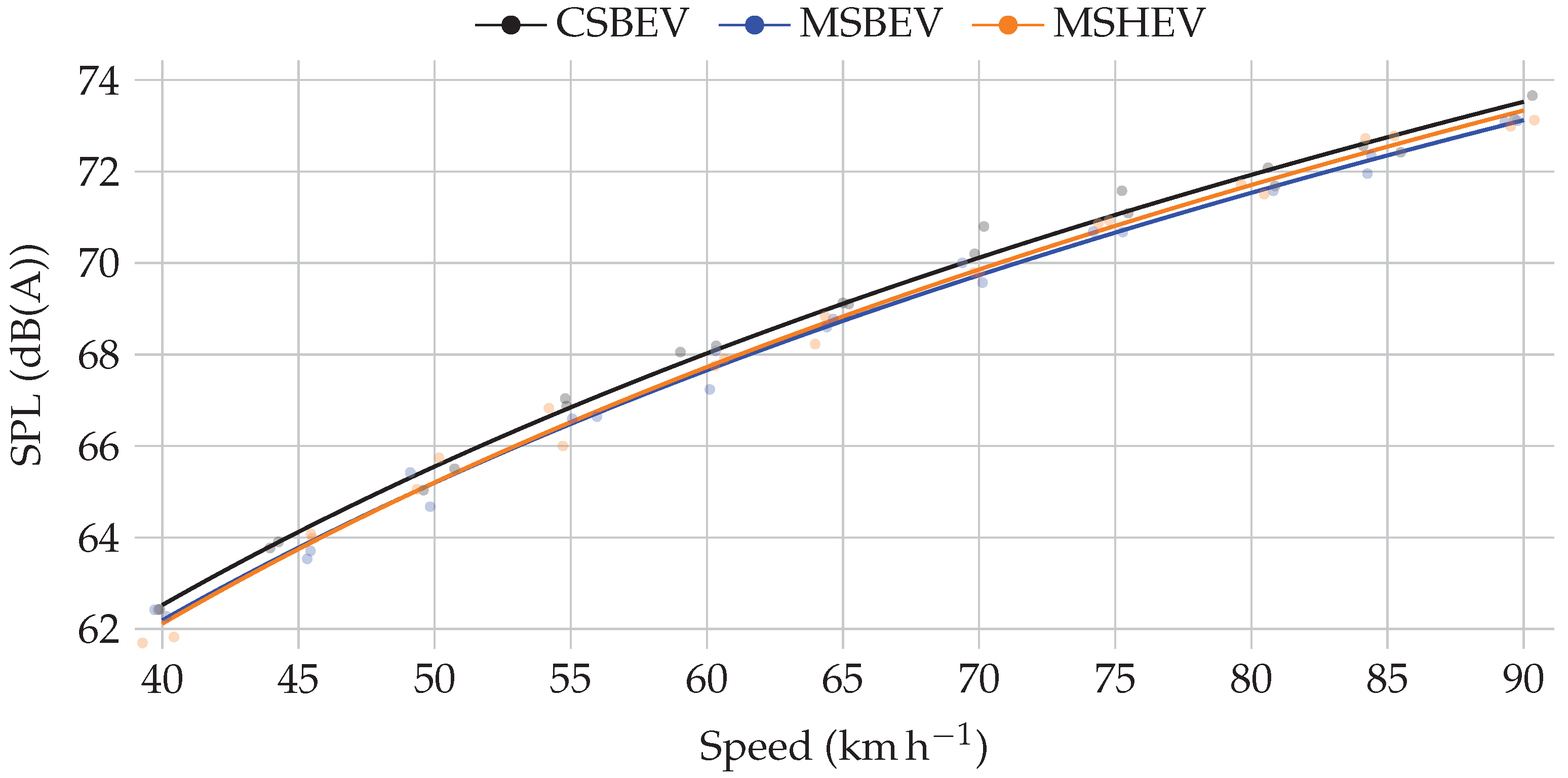
The second block in the DoE includes a Hankook Ventus S1 Evo3 of the size 255/45 R19 measured on two different EVs (CSBEV, MSBEV) as well as one hybrid vehicle with ICE (MSHEV). All measurements are conducted in an air temperature range of 12.1 °C to 12.8 .
5.3.1. Rolling Noise—Vehicle impact
In case of the rolling noise, measured with the vehicle with ICE, the engine remained switched on while driving in idle mode through the test track.
As Figure 11 shows, there is a slight difference in rolling noise of each vehicle. While the average absolute difference between CSBEV and MSBEV is dB(A), the average absolute difference between MSBEV and MSHEV is dB(A) and between CSBEV and MSHEV dB(A). For these values the MB-Correction is already applied. Since the average absolute differences are rather small and the regression curves all reach CODs of , it is not wise to assume that the differences are solely due to measurement error. Even though the larger EV weighs 2500 and the lighter one 2140 , the heavier one reaches a smaller SPL. That observation is rather astonishing since a lot of research exists that leads to the conclusion that higher loads on the tire cause higher SPLs ((Sandberg and Ejsmont [6] pp. 195–200) gives an overview of according research).

Figure 11.
Air temperature corrected rolling SPL regression curves compared on three different vehicles for 255H on the left microphone.
Nevertheless, the suspected weight-induced increase in the SPL, assuming linearity in the assumption of the Ph.D. thesis mentioned in the introduction, should be around dB(A) (Ref. [6] cited from Taryma Stansilaw (Thesis from Taryma Stansilaw from 1982, due to original language not available to author). Because in this measurement series, the vehicles that are only slightly different in their shape (especially in axle distance as well as wheel base) almost lead to the same SPL, the assumption is plausible that shape parameters do matter more than weight variations.
5.3.2. Accelerated Noise—Vehicle Impact
In case of the 255H mounted on the EVs, the accelerated noise increase is displayed in Figure 12.
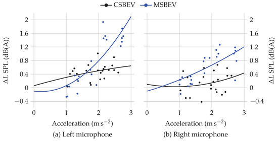
Figure 12.
Accelerated noise behavior of the tire 255H on two different EVs.
The figure shows that the impact of different vehicles on additional accelerated noise is large, at least for higher accelerations than 2 . The average additional SPL for all runs over that acceleration is 1 (A) higher in case of the MSBEV than for the CSBEV. Below this acceleration, the mean for the CSBEV is dB(A) higher. Furthermore, it is noticeable that the curve received for the CSBEV on the microphone to the left side of the vehicle is concave. Nevertheless, there is no recording in the literature of similar behavior, and thus this is also presented in this research only here. In the case of 255P in AWD at the right microphone, and 255B on MSBEV at the right microphone the case, no reasonable explanation applies.
5.4. Bridgestone Turanza T005
The largest block in the DoE consists of a Bridgestone Turanza T005 mounted on five different vehicles, from which three are EVs (CSBEV, MSBEV, LSBEV). Thereby, the variation in rolling noise caused by vehicles as well as weight adaptions and the impact on accelerated noise due to different vehicles is investigated.
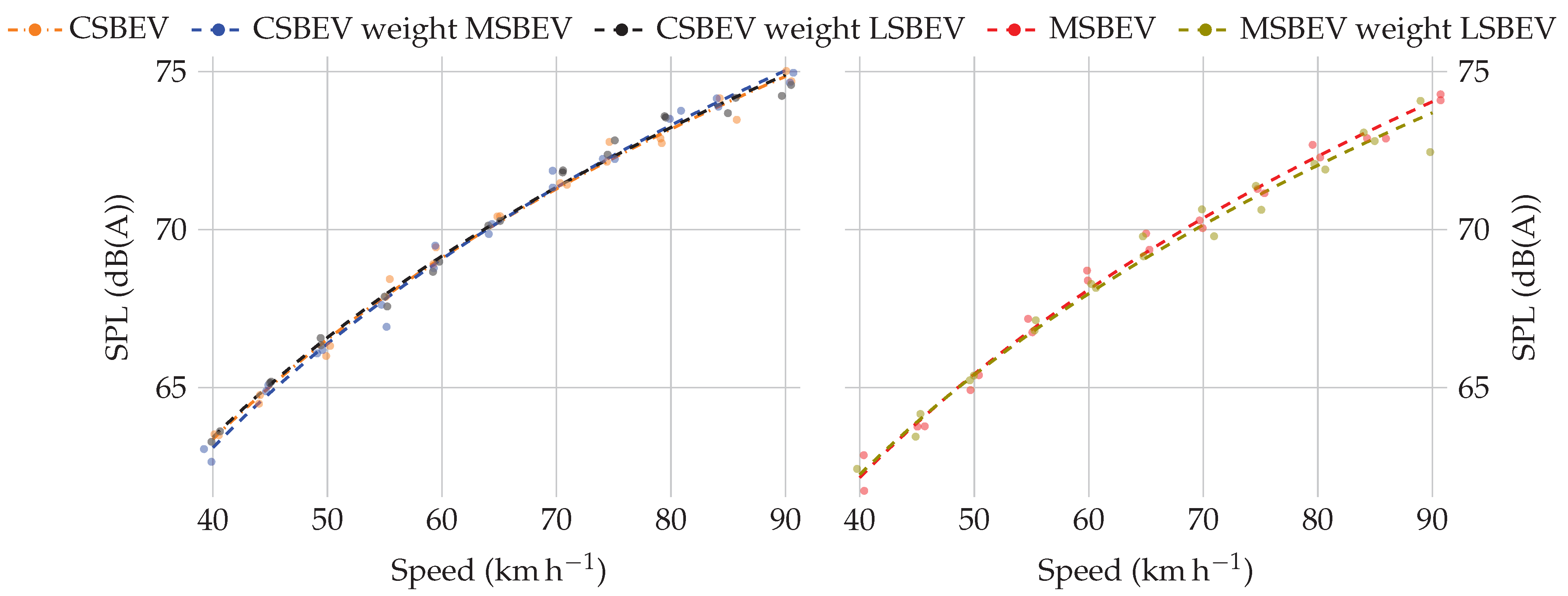
5.4.1. Rolling Noise—Vehicle Impact and Weight Variation
Figure 13 shows a total of five measurements with three weight variations. The weight adaption is received through bags of stone granulate that are fixed in the vehicle. In case of the CSBEV an overall difference of 11 and wheel wise difference of 24 is achived. In case of the MSBEV as LSBEV, the overall difference is 37 and wheel wise difference varies from −35 to 65 . In the left diagram, a weight adaption of the CSBEV to an MSBEV only leads to an average deviation of dB(A). In the case of weight adaption to LSBEV of dB(A). The MSBEV as LSBEV leads to an average absolute difference of dB(A). Since the additional weight from MSBEV to LSBEV is (104 ) and the additional weight necessary for CSBEV to LSBEV is (474 ), it is to assume that the recorded differences are purely statistic measurement errors. Otherwise, the highest average absolute error would be recorded between CSBEV and CSBEV as LSBEV. This supports the previous assumption that in this range of vehicle’s weights, it does not have an influence.
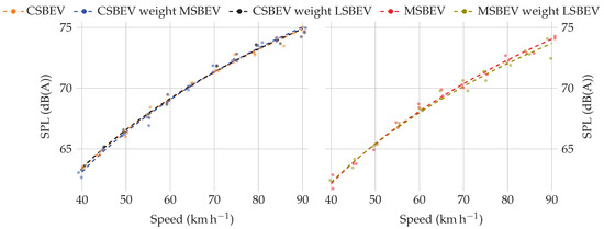
Figure 13.
Air temperature corrected rolling SPL regression curves compared on CSBEV and MSBEV with different added weight on the left microphone.
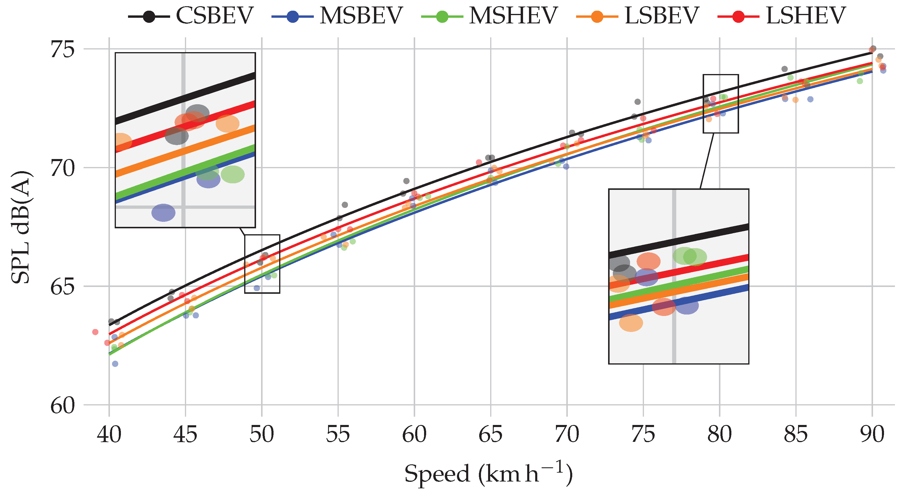
Since the weight adaption did not show a difference in the SPLs, the weight variations can be neglected in the following results. Figure 14 shows the overall vehicle impact on rolling noise after temperature correction. To illustrate the difference between the curves more precisely, the most important areas are magnified. The areas respond to the necessary constant run at 50 in [2] and the tire noise label that is calculated through a linear regression for 80
according to UN/ECE Regulation No. 117 [19].

Figure 14.
Air temperature corrected rolling SPL regression curves compared on five different vehicles for 255B on the left microphone.
As recorded in Section 5.3.1, there is an impact of the vehicle shape and parameters on the rolling noise. The 255H as well as the 255B lead to the same observation that the smaller EV CSBEV is louder than the MSBEV. In the case of the Bridgestone, the average absolute difference is dB(A). Furthermore, it is notable that the average absolute error is always minimal when the vehicle shapes are almost identical. In the case of the MSHEV, this means that the closest curve can be found with the MSBEV and an average absolute error of dB(A). For the LSHEV, the closest other vehicle is the LSBEV with an average absolute error of dB(A).
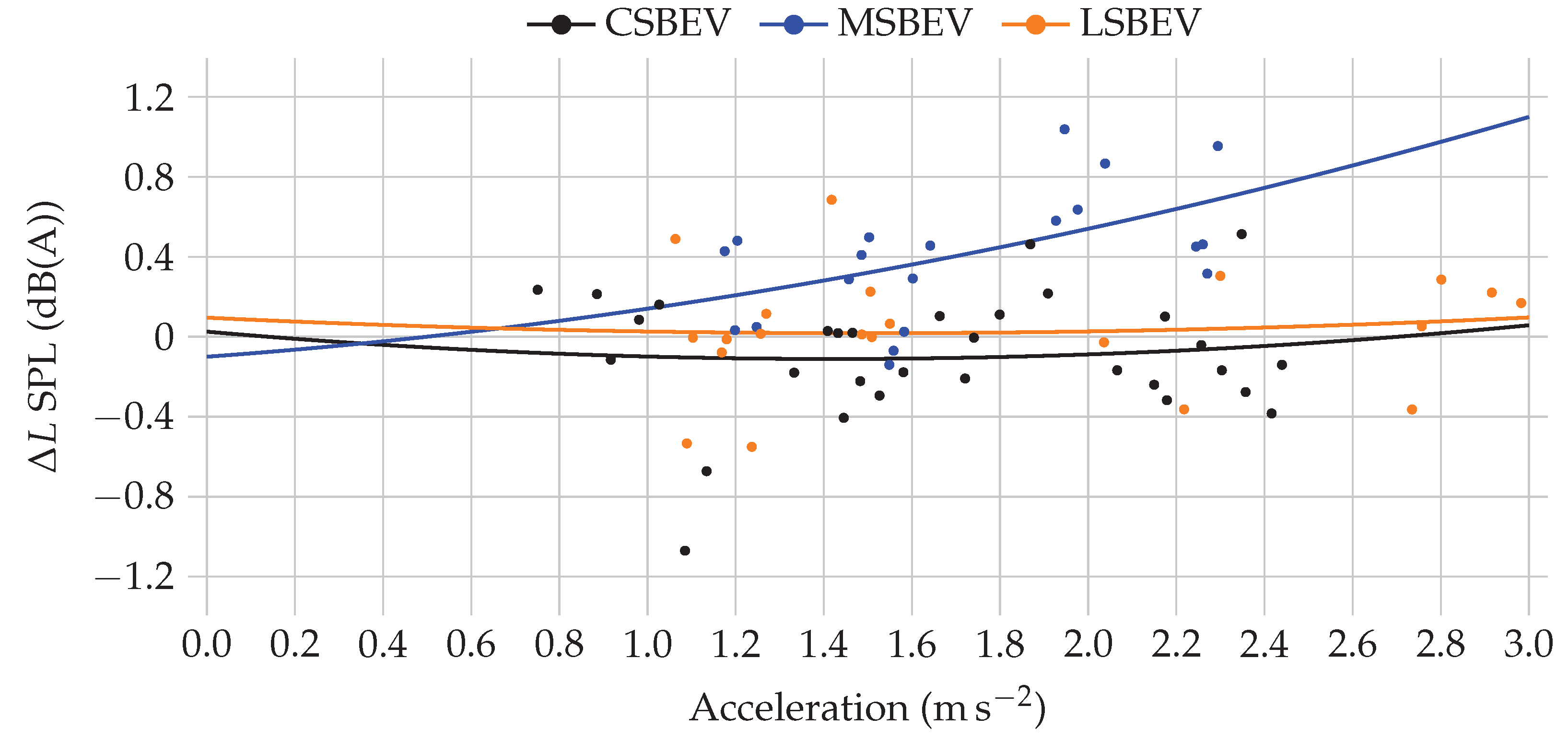
5.4.2. Accelerated Noise—Vehicle Impact
Figure 15 shows the accelerated noise of the 255B mounted on three different EVs. Identical to the results presented in Section 5.3.2, the impact of the vehicle for accelerated tire behavior does not seem to be large below 2 . Furthermore, it is notable that the MSBEV leads to a greater slope than the CSBEV and LSBEV. This is also in accordance with previous results. Nevertheless, it is possible to state that it is questionable whether the recorded data is impacted by the vehicle acceleration, or if the data points are primarily statistical measurement errors.
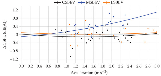
Figure 15.
Accelerated noise behavior of the tire 255B on three different EVs.
5.5. Error Evaluation
In some cases, the difference between the calculated regression curves for the rolling noise is small, especially compared to the absolute SPL. That leads to the question of general measurement errors and therefore, whether the observed difference is rather a statistical measurement error, defined by, e.g., calibration error, measurement accuracy, and environmental conditions, as well as the attempt to correct these.
To get closer insights in the measurement dispersion and plausibility of the previously displayed results, in one scenario the 50 idle drive is repeated 10 times. The results are shown in Figure 16, the dashed line indicates the average SPL, which happens to be identical to the second decimal for both sides. It is important to acknowledge that the error seems to be Gaussian distributed and centered on the mean of the measurements. The right side shows the distributions obtained for each side. These are calculated through a kernel density approach. Thereby, a Gaussian kernel with a bandwidth of is used.
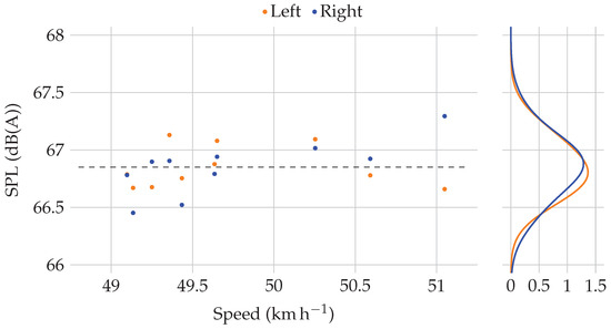
Figure 16.
SPL and their distributions at Point P-P’ for idle runs at approximately 50/ for microphones on right and left side.
The maximal recorded spread between the measurements is dB(A) on the left and dB(A) on the right side. As already indicated by the probability distribution, the standard deviations are much lower with dB(A) and dB(A) for left and right side. Even though an absolute error of dB(A) would be rather high, by always repeating the same driving conditions at least twice, the accuracy of the overall measurement and therefore regression curve is higher.
6. Tire Changing Algorithm
As hinted in the introduction, the tire change has two purposes: to reduce the overall necessary measurements and enable measurements on the test bench where the tire noise can not be simply recorded. The second aspect is also very important since using a test bench makes it possible to rule out all environmental impact on the recorded SPLs and therefore makes it a very useful tool to compare standardised measurements. For the following results, the accelerated coefficients are calculated with the least square approach. This is decided since this is the standard algorithm implemented in common measurement software. Section 4 showed that in the area of driven accelerations there is almost no difference resulting from the used algorithms.
Figure 17 shows the principle behind the virtual tire change. Two different tires are measured on a specific test track, using a silent ICE vehicle or EV to calculate the five regression coefficients that describe the tire noise. These coefficients describe the overall tire noise emitted depending on speed as well as acceleration. They are only valid if the distance between tire and microphone remains the same. Since this is not possible on a pass-by measurement, the coefficients are calculated for each point of the test track, leading to a coefficient matrix. This matrix can be multiplied with a driving dynamic (speed and acceleration over distance) of a vehicle measurement according to, e.g., UN/ECE 40 Regulation No. 51 [2], where an ICE is used at full throttle. That leads to an SPL curve over the track distance that purely describes the anticipated tire noise. By subtracting this curve from the raw measurement and adding a second tire curve, a virtual tire change is performed.
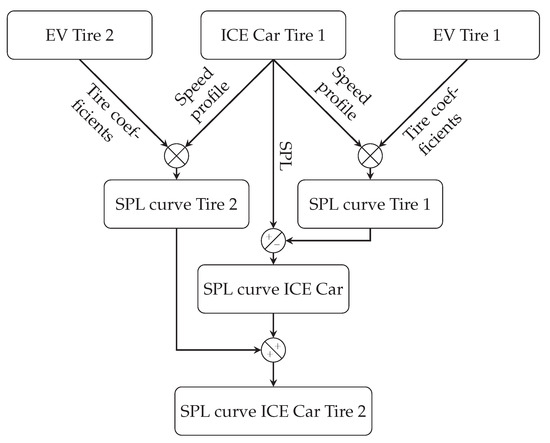
Figure 17.
Principal sketch of tire changing algorithm.
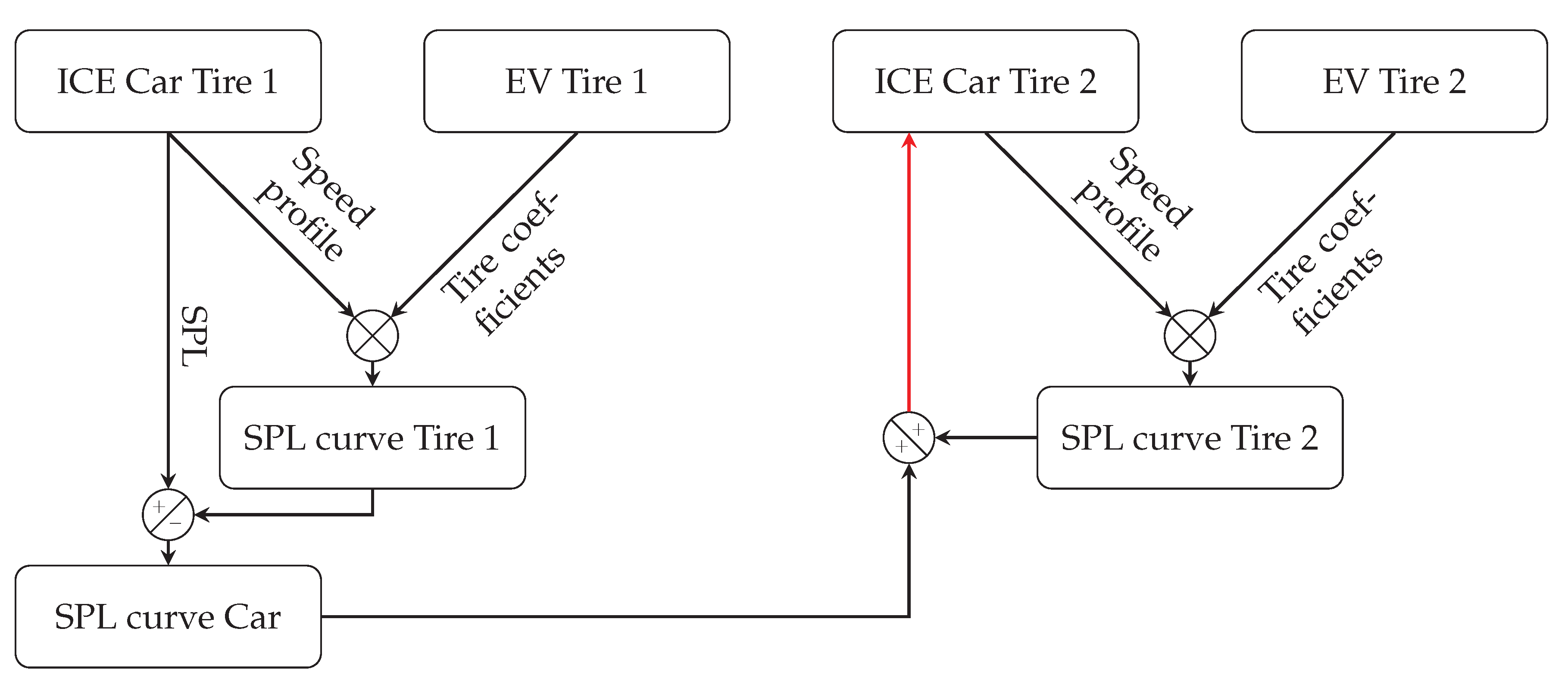
Figure 18 illustrates how the tire change can be validated. In essence, to validate the algorithm, at least four measurements are necessary. Two must be a measurement of solely tire noise and two must be measurements with ICE with one specific vehicle and the same tires as in the first two measurements. Both speed profiles should be approximately the same so that no difference in the exhaust and engine noise curves must be expected. The gear should also be the same since switching the gear at the same driving speed has a huge impact on engine and exhaust noise level and frequency.
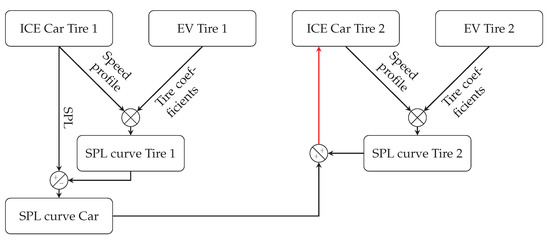
Figure 18.
Principal sketch of validation of tire changing algorithm.
In essence, the result of the red colored arrow is compared to the SPL of the reference measurement. The measurements conducted in this research allow the validation for multiple tire and car combinations. Thereby, the comparison is undertaken for two single runs of the vehicle with ICE, each one with a different tire.
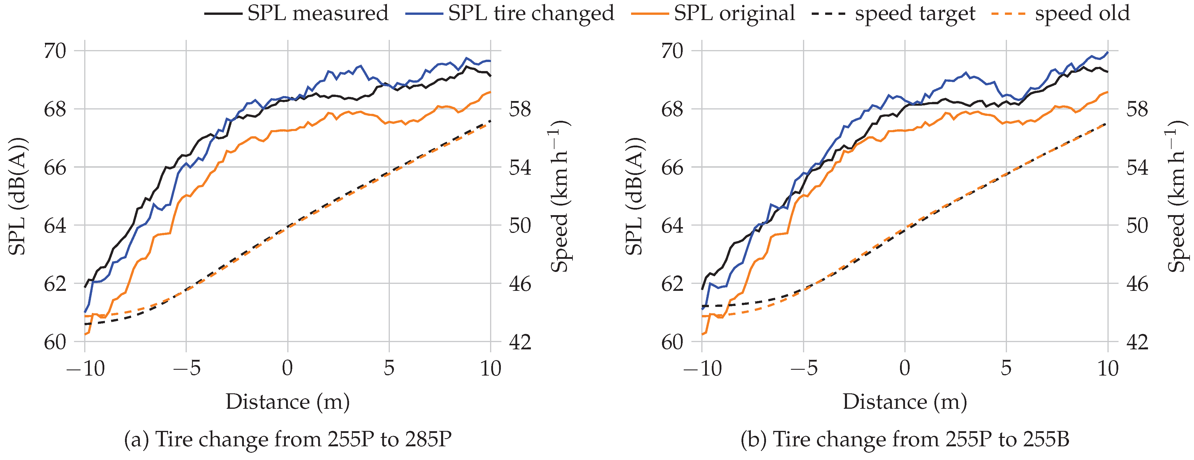
Figure 19 shows the achieved curves for two different tire changes. The subtracted tire is both times the 255P and the tire change is performed for an LSHEV driven in sports mode to ensure that engine and exhaust noise is not negligible. In Figure 19a the tire is changed to the 285P, in Figure 19b to the 255B. The speed profiles are also included as well as the original SPL curve from the LSHEV with the 255P mounted. For both cases, the changing algorithm seems to over exaggerate the total noise, especially in the area of maximum noise. The improvement of changing the tire is already optically visible in case of the two 285P being changed. The average absolute error decreases from dB(A) to dB(A). For the change from 255P to 255B the average absolute error decreases from dB(A) to dB(A).
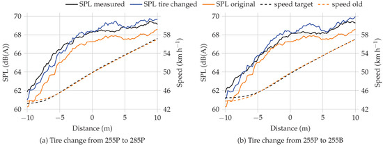
Figure 19.
Tire change for LSHEV, tires measured while mounted on LSBEV, pred indicating the EV used for the prediction.
The results presented in Figure 19 are conducted through calculating the tire coefficients using measurements from an LSBEV. This vehicle is, in Section 5.4, observed to lead to the closest coefficients as the LSHEV for the rolling coefficients. That begs the question whether it is important for which vehicle the tire coefficients are calculated or if the EV’s impact cancels out if both tires are measured on the same one. To answer that, question, Figure 20 shows three curves for three different tire changes. The tires are changed from 255B to 255H, with different EVs used to calculate the tire coefficients. The different scenarios are as follows. MSBEV used for subtraction and addition, CSBEV used as subtraction and addition, and LSBEV used for subtraction with MSBEV used as addition. As the figure shows, the original curves of the MSHEV are rather similar with an average absolute error of dB(A). Nevertheless, especially in the first 4 of the test track all of the changed curves have smaller deviation from the SPL curve of MSHEV with 255H than the MSHEV SPL curve without tire change (255P). On the remaining part of the test track, this trend changes. Here, only the tire change through measurements conducted with the MSBEV seem to lead to better results than no tire change. The average absolute errors, CSBEV dB(A), MSBEV dB(A), and LSBEV dB(A) indicate that any change would be better than no change. Nevertheless, that is not really true since, for the certification of vehicles, the overall maximum SPL is relevant and that is overestimated in the case of the LSBEV by dB(A) and underestimated in the case of the CSBEV by dB(A).
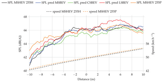
Figure 20.
Tire change for MSHEV, tires measured while mounted on different EVs, pred indicating the EV used for the prediction.
Taking a look at the results in Section 5 and Section 6, it is to assume that the used EV to calculate the regression coefficients does indeed have an impact on the tire changing algorithm. Thereby, vehicles with comparable outer shapes lead to the most accurate results in the tire changing algorithm.
7. Discussion and Outlook
The measurement series presented in Section 5 and Section 6 lead to the following six main conclusions that extend or question the existing literature.
Firstly, the vehicle weight does not seem to have any noticeable impact. That is what measurements for a weight difference of up to one quarter of the absolute weight indicate. This contradicts the literature presented in Section 1.
Secondly, the accelerated noise increase depends on the applied torque on the wheels rather than the vehicle acceleration. This assumption is reasonable since in the cases where torque is only applied on two rather than four wheels, the slopes of regression curves are larger and increase more rapidly. This results in two louder sources that lead to an absolute louder noise than four less noisy sources. The maximum recorded increase in SPL due to acceleration lower than 2 was recorded with dB(A).
Thirdly, some of the tires investigated in this research emit less noise for small accelerations compared to no acceleration.
Fourthly, the rolling noise of mixed mounted tires can be approximated by averaging the rolling noise of the two measurements with according equal tires. In case of the accelerated noise and mixed mounted tires, the non-accelerated tire also has a small impact on the calculated regression curve.
Fifthly, the rolling noise is impacted by the choice of vehicle up to an average absolute difference of approximately 1 dB(A).
Finally, the virtual tire change does seem to lead to overall good results with a slight restriction that the vehicle body shape seems comparable. Nevertheless, it is notable that the presented tire changes are only single runs that are compared. The fact that even these single, repeated runs can lead to very different SPL curves makes it assumable that the tire change generally works even better since, through trying to generate a validation run, some error is inserted in the algorithm.
Overall, this research confirms that the virtual tire change works, and that at least for AWD the acceleration of tires does not have a large impact on the SPL relevant for certification according to UN/ECE Regulation No. 51 [2].
More research needs to be conducted to solve the question of why some vehicles lead to larger rolling noise. These topics might also be addressed on test benches, since in that way all environmental conditions could be standardised. In addition, more research is necessary to determine why some tires do not seem to fit the generalized accelerated behavior. Thereby, it is also necessary to validate that the torque leads to higher CODs than the acceleration.
Author Contributions
Conceptualization, M.L., F.G.; methodology, M.L.; software, M.L.; validation, M.L.; investigation, M.L.; data curation, M.L.; writing—original draft preparation, M.L.; writing—review and editing, M.L. and F.G.; visualization, M.L.; supervision, F.G.; project administration, M.L. All authors have read and agreed to the published version of the manuscript.
Funding
This research received funding by Mercedes-Benz Group AG.
Acknowledgments
The authors thank the Mercedes-Benz Group AG with the department overall vehicle integration NVH powertrain for their support. Additionally the authors thank Timo von Wysocki from the department overall vehicle integration NVH carbody and chassis for always being available to discuss the ongoing research. The authors thank Achim Winandi from the Karlsruhe Institute of Technology for valuable input and support. We acknowledge support by the KIT-Publication Fund of the Karlsruhe Institute of Technology.
Conflicts of Interest
The authors declare no conflict of interest. Michael Leupolz is from Mercedes-Benz Group AG, the company had no role in the design of the study; in the collection, analyses, or interpretation of data; in the writing of the manuscript, and in the decision to publish the results.
Abbreviations
The following abbreviations are used in this manuscript:
| SPL | Sound Pressure Level |
| ICE | Internal Combustion Engine |
| EV | Electric Vehicle |
| BEV | Battery Electric Vehicle |
| HEV | Hybrid Electric Vehicle |
| COD | Coefficient of Determination |
| CSBEV | Compact SUV Battery Electric Vehicle |
| MSBEV | Midsize SUV Battery Electric Vehicle |
| LSBEV | Luxury Sedan Battery Electric Vehicle |
| MSHEV | Midsize SUV Hybrid Electric Vehicle |
| LSHEV | Luxury Sedan Hybrid Electric Vehicle |
Appendix A
Table A1.
List of abbreviations tire combinations.
Table A1.
List of abbreviations tire combinations.
| Abbreviation | Translation |
|---|---|
| 255P | 255/40 R20 Pirelli PZero |
| 285P | 285/35 R20 Pirelli PZero |
| 255P + 285P | 255/40 R20 Pirelli PZero front axle + 285/35 R20 Pirelli PZero rear axle |
| 255B | 255/45 R19 Bridgestone Turanza T005 |
| 255H | 255/45 R19 Hankook Ventus S1 Evo3 |
Table A2.
Experiment design without weight adaption.
Table A2.
Experiment design without weight adaption.
| Tires | CSBEV | MSBEV | LSBEV | MSHEV | LSHEV |
|---|---|---|---|---|---|
| 255P | - | - | X | - | X |
| 255P + 285P | - | - | X | - | - |
| 255H | X | X | - | X | - |
| 255B | X | X | X | X | X |
Table A3.
Experiment design weight adaption.
Table A3.
Experiment design weight adaption.
| Weight of | CSBEV | MSBEV |
|---|---|---|
| MSBEV | 255B | - |
| LSBEV | 255B | 255B |
References
- Noise and Health: Report by a Committee of the Health Council of the Netherlands; Publication/Gezondheidsraad, Health Council of The Netherlands: The Hague, The Netherlands, 1994.
- UN/ECE Regulation No. 51. Uniform Provisions Concerning the Approval of Motor Vehicles Having at Least Four Wheels with Regard to Their Sound Emissions [2018/798]. Available online: https://eur-lex.europa.eu/legal-content/EN/TXT/?uri=CELEX%3A42018X0798 (accessed on 8 April 2022).
- Putner, J.; Lohrmann, M.; Fastl, H. Contribution analysis of vehicle exterior noise with operational transfer path analysis. Proceedings of Meetings on Acoustics ICA2013, Montreal, QC, Canada, 2–7 June 2013; Volume 19, p. 040035. [Google Scholar]
- Zeller, P. (Ed.) Handbuch Fahrzeugakustik: Grundlagen, Auslegung, Berechnung, Versuch, 3rd ed.; Springer: Wiesbaden/Heidelberg, Germany, 2018. [Google Scholar] [CrossRef]
- Jabben, J.; Verheijen, E.; Potma, C. Noise reduction by electric vehicles in the Netherlands. In INTER-NOISE and NOISE-CON Congress and Conference Proceedings; Institute of Noise Control Engineering: Lisbon, Portugal, 2012; pp. 6958–6965. [Google Scholar]
- Sandberg, U.; Ejsmont, J.A. Tyre/Road Noise: REFERENCE Book, 1st ed.; INFORMEX Ejsmont & Sandberg Handelsbolag: Kisa, Sweden, 2002. [Google Scholar]
- DIN ISO 362-3:2021-11; Messverfahren für das von beschleunigten Straßenfahrzeugen abgestrahlte Geräusch–Verfahren der Genauigkeitsklasse 2—Teil 3: Indoor-Prüfung der Klassen M und N (ISO 362-3:2016). Beuth Verlag GmbH: Berlin, Germany, 2011.
- Ejsmont, J.A.; Sandberg, U. Influence on Tire/Road Noise Emission by Vehicles of Different Construction; VTI: Linköping, Sweden, 1990. [Google Scholar]
- Ejsmont, J.A.; Mioduszewski, P.; Taryma, S.; Sandberg, U. Tire/Road Noise Emission and Its Measurement: Effects of Rim and Other Objects Close to the Tire, Such as Enclosure and Wheel Housing; VTI: Linköing, Sweden, 1996. [Google Scholar]
- Stalter, F.; Frey, M.; Gauterin, F. Einfluss des Antriebsmoments auf das Reifengeräusch. ATZ Automob. Z. 2013, 115, 528–533. [Google Scholar] [CrossRef]
- Grollius, S.; Gauterin, F. Experimentelle Untersuchung zum Einfluss des Antriebsmoments auf das Reifen-Fahrbahn-Geräusch. In Verbundprojekt Leiser Straßenverkehr 2, Berichte der Bundesanstalt für Straßenwesen; BASt: Bergisch Gladbach, Germany, 2012; pp. 48–67. [Google Scholar]
- Hoever, C.; Tsotras, A.; Pallas, M.A.; Cesbron, J. Einfluss von Reifen- und Betriebsparametern auf das Reifen-/Fahrbahngeräusch unter Drehmoment: Presentation Slides. Fortschritte der Akustik - DAGA 2022. Available online: https://www.dega-akustik.de/publikationen/online-proceedings/ (accessed on 25 April 2022).
- Hoever, C.; Tsotras, A.; Pallas, M.A.; Cesbron, J. Einfluss von Reifen- und Betriebsparametern auf das Reifen-/Fahrbahngeräusch unter Drehmoment. Fortschritte der Akustik-DAGA. 2022, pp. 451–454. Available online: https://www.dega-akustik.de/publikationen/online-proceedings/ (accessed on 25 April 2022).
- Li, T.; Burdisso, R.; Sandu, C. The effects of tread patterns on tire pavement interaction noise. In INTER-NOISE and NOISE-CON Congress and Conference Proceedings; Institute of Noise Control Engineering: Lisbon, Portugal, 2016; Volume 253, pp. 208–219. [Google Scholar]
- Ejsmont, J.A.; Sandberg, U.; Taryma, S. Influence of tread pattern on tire/road noise. SAE Trans. 1984, 93, 632–640. [Google Scholar]
- Sandberg, U. Road traffic noise—The influence of the road surface and its characterization. Appl. Acoust. 1987, 21, 97–118. [Google Scholar] [CrossRef]
- Liao, G.; Sakhaeifar, M.S.; Heitzman, M.; West, R.; Waller, B.; Wang, S.; Ding, Y. The effects of pavement surface characteristics on tire/pavement noise. Appl. Acoust. 2014, 76, 14–23. [Google Scholar] [CrossRef]
- Vázquez, V.F.; Terán, F.; Paje, S.E. Dynamic stiffness of road pavements: Construction characteristics-based model and influence on tire/road noise. Sci. Total Environ. 2020, 736, 139597. [Google Scholar] [CrossRef] [PubMed]
- UN/ECE Regulation No. 117. Uniform Provisions Concerning the Approval of Tyres with Regard to Rolling Sound Emissions and to Adhesion on Wet Surfaces and/or to Rolling Resistance. Available online: https://eur-lex.europa.eu/legal-content/DE/TXT/?uri=CELEX%3A42011X1123%2803%29 (accessed on 8 April 2022).
- Savitzky, A.; Golay, M.J.E. Smoothing and differentiation of data by simplified least squares procedures. Anal. Chem. 1964, 36, 1627–1639. [Google Scholar] [CrossRef]
- DIN EN 61672-1:2014-07; Elektroakustik—Schallpegelmesser—Teil 1: Anforderungen (IEC 61672-1:2013); Deutsche Fassung EN 61672-1:2013. Beuth Verlag GmbH: Berlin, Germany, 2014.
- Ruppert, D.; Wand, M.P. Multivariate locally weighted least squares regression. Ann. Stat. 1994, 22, 1346–1370. [Google Scholar] [CrossRef]
- Boyd, S.P.; Vandenberghe, L. Introduction to Applied Linear Algebra: Vectors, Matrices, and Least Squares; Cambridge University Press: Cambridge UK; New York, NY, USA, 2018. [Google Scholar]
- Chen, Y.C. A tutorial on kernel density estimation and recent advances. Biostat. Epidemiol. 2017, 1, 161–187. [Google Scholar] [CrossRef]
- Steininger, M.; Kobs, K.; Davidson, P.; Krause, A.; Hotho, A. Density-based weighting for imbalanced regression. Mach. Learn. 2021, 110, 2187–2211. [Google Scholar] [CrossRef]
- Węglarczyk, S. Kernel Density Estimation and Its Application; ITM Web of Conferences: Les Ulis, France, 2018; Volume 23, p. 00037. [Google Scholar]
- Virtanen, P.; Gommers, R.; Oliphant, T.E.; Haberland, M.; Reddy, T.; Cournapeau, D.; Burovski, E.; Peterson, P.; Weckesser, W.; Bright, J.; et al. SciPy 1.0: Fundamental Algorithms for Scientific Computing in Python. Nat. Methods 2020, 17, 261–272. [Google Scholar] [CrossRef] [PubMed] [Green Version]
- Stalter, F.C. Ansätze zur akustischen Optimierung von Reifen und Fahrbahnen für Elektrofahrzeuge unter Antriebsmoment. Ph.D. Thesis, Karlsruhe Institue of Technology, Karlsruhe, Germany, 2016. [Google Scholar]


Publisher’s Note: MDPI stays neutral with regard to jurisdictional claims in published maps and institutional affiliations. |
© 2022 by the authors. Licensee MDPI, Basel, Switzerland. This article is an open access article distributed under the terms and conditions of the Creative Commons Attribution (CC BY) license (https://creativecommons.org/licenses/by/4.0/).