Computational Study of the Plasma Actuator Flow Control for an Airfoil at Pre-Stall Angles of Attack

Abstract

Large-eddy simulations of the flows over an NACA0015 airfoil were conducted to investigate a flow control authority of a dielectric barrier discharge plasma actuator at pre-stall angles of attack. The Reynolds number was set to 63,000, and angles of attack were set to 4, 6, 8, and 10 degrees. The plasma actuator was installed at 5% chord length from the airfoil’s leading edge. Good flow control authority was confirmed in terms of lift-to-drag ratio increase and drag reduction. These improvements mainly result from the reduction of the pressure drug, which is due to the change in pressure distribution accompanying the movement and shrink of the laminar separation bubble on the airfoil surface. Additionally, although flow control using a burst drive with a nondimensional burst frequency of six improves the lift-to-drag ratio at all angles of attack, the phenomena leading to the improvement differ between near-stall angles (10 and 12 degrees) and the other lower angles. At near-stall angles, the turbulent transition is rapidly promoted by PA, and the flow is reattached. Whereas, at the lower angles, the transport of two-dimensional vortex structures, which maintain their structures up to downstream and suppress the turbulent transition, makes the flow reattachment.

1. Introduction

Flow control using a dielectric barrier discharge plasma actuator (PA) has been widely studied for the last 10 to 20 years because PA has the advantages of thin/light simple structures and easy to use. PA only consists of two electrodes with a dielectric layer between them (Figure 1), and can be attached to an existing body surface without changing the original shape of the body surface. PA can be attached on flat or curved surfaces, corners, or edges and flow separation is controlled [1,2,3]. PA is also used for the control of boundary layer flows [4,5,6,7,8,9] and many researchers have tried to reduce skin friction drag by PA. To enhance the authority of PA, studies for PA expand over wide areas of research: low-temperature plasma discharge, flow structures induced by PA, use of duty cycles, etc. Geometry of the electrodes and the layout of multiple PAs were also studied. A good review of different types of PAs was written by Wang, Choi, and others [10], where review papers for conventional use of flow control by PA were presented. Up to the present, there has been active research on the application of various types of PA in a variety of devices [11,12,13].

For the flow separation control over an airfoil, PA is installed near the leading edge on the suction side of the airfoil surface except for in a few cases [14]. Most of the studies used a two-dimensional spanwise electrode, which induces coherent spanwise jet flows. Some studies used effective duty cycles (so-called burst actuation compared to regular continuous actuation), where still more effective flow control is achieved by a proper choice of the PA parameters. When duty cycles are used, two-dimensional coherent discrete vortex structures are induced at every cycle of the duty. Thus, PAs—especially in the burst actuation—have three important flow features: jet flow near the airfoil surface, two-dimensional vortex structures with the merger of these structures, and introduction of flow disturbances. Good authority of PA comes from the fact that each of these features may become dominant with proper choice of electric parameters [15]. Furthermore, in the flow control for airfoil flows, saw-tooth, serpentine spanwise electrodes, or line up of the chordwise electrodes—which create chordwise vortex structures and others—were studied by several authors [16,17,18,19].

In either case, most of the former studies were conducted at post-stall angles of attack [4,20,21,22] and lift characteristics were mainly discussed since interest was in the control of the separated shear layer over an airfoil. Effective parameters of PA, such as locations, burst frequencies, and others, were discussed both computationally and experimentally. Although computational studies showed that drag reduction [23] occurred in many cases, the mechanism of the drag reduction was not well discussed. From the observation of the flow fields computationally simulated by the present authors’ group, pressure drag was identified to be the main source of drag reduction for the flows at the Reynolds number of order of ${10}^4$ to ${10}^5$, where laminar separation bubbles play an important role for the airfoil aerodynamic characteristics. Since laminar separation bubbles exist at angles of attack lower than the stall, we may expect a similar drag reduction even at pre-stall angles of attack. UAV or MAV would be considered for the application of flow control by PA at this Reynolds number range. Atmospheric wind would influence much for the flow conditions for these type of flight vehicles, and it is necessary to understand flow features and achieve high $L/D$ for a wide range of angles of attack, and discuss flow control authority of PA. Several researchers investigate the flow at pre-stall angles of attack [24,25,26], but most of their work is aimed at evaluating aerodynamic characteristics, and analysis of the flow feature is not their major focus.

Regarding pre-stall conditions, we have conducted two types of computational studies in the past. First, we showed that better $L/D$ (lift-to-drag ratio) is obtained at cruise conditions than that of the well-recognized airfoil geometry [27]. Here, the detailed flow structure was discussed, but for only a single angle of attack $\alpha =6$ deg. The result indicated that burst actuation tends to keep sequential spanwise vortex structures over the upper surface and keeps flow laminar until near the trailing edge in contrast to the promotion of turbulent transition at near stall angle [15]. The resultant flow field became similar to the flow over a well-recognized high-performance airfoil at a low Reynolds number flow regime. Second, a survey of several angles of attack was carried out [28]. Here, time-averaged aerodynamic characteristics were mainly discussed, and unsteady flow features were not discussed in conjunction with the aerodynamic characteristics at each angle of attack.

The present study aims to understand the PA-controlled flow features by performing high-fidelity LESs at a broader range of pre-stall angles of attack and discuss the relation with the aerodynamic characteristics of the airfoil. The flow fields over an NACA0015 airfoil at angles of attack $\alpha =$ 4, 6, 8, and 10 deg are considered. NACA0015 airfoil flows have been investigated in many previous studies [8,23,29,30,31], and a wealth of experimental and numerical data are available for comparison. The thickness of this airfoil is not practical for actual flights. However, such a thick airfoil is less restrictive in structural design and has the advantage that a large amount of fuel can be loaded inside a wing. Therefore, the range of aircraft design possibilities will expand if the flow controls can improve the aerodynamic characteristics. The Reynolds number was set to 63,000, which was considered in the previous experimental and computational studies [8,29,30,32], and reliability of the flow simulations has been well established. Previous studies [8,30] show that small fluid fluctuations such as turbulence play an important role in fluid control using PA. In the Reynolds-averaged Navier–Stokes equation (RANS) method, the small fluctuations induced by PA are immediately damped. Therefore, in the present study, wall-resolved LESs are conducted to resolve small fluid fluctuations properly. The obtained results are discussed together with the result of the post-stall condition ($\alpha =12$).

Throughout the obtained results, the flow fields and the relationship between the aerodynamic characteristics are discussed. Focus is laid on the drag reduction, but the lift and the lift-to-drag ratio are also discussed. The results show the good flow control authority of PA for the aerodynamic characteristics of the airfoil at pre-stall angles of attack. In the cases of burst actuation, although the aerodynamic characteristics are improved at all angles of attack, the phenomena leading to the improvement are different between near-stall angles (including the post-stall angle) and lower angles. At near-stall angles, the turbulent transition is rapidly promoted by PA, and the flow is reattached. Whereas, at lower angles, the transport of two-dimensional vortex structures, which maintain their structures downstream and suppresses the turbulent transition, allow the flow reattachment. Furthermore, the strategy of parameter settings of burst actuation of PA at angles of attack less than stall is indicated.

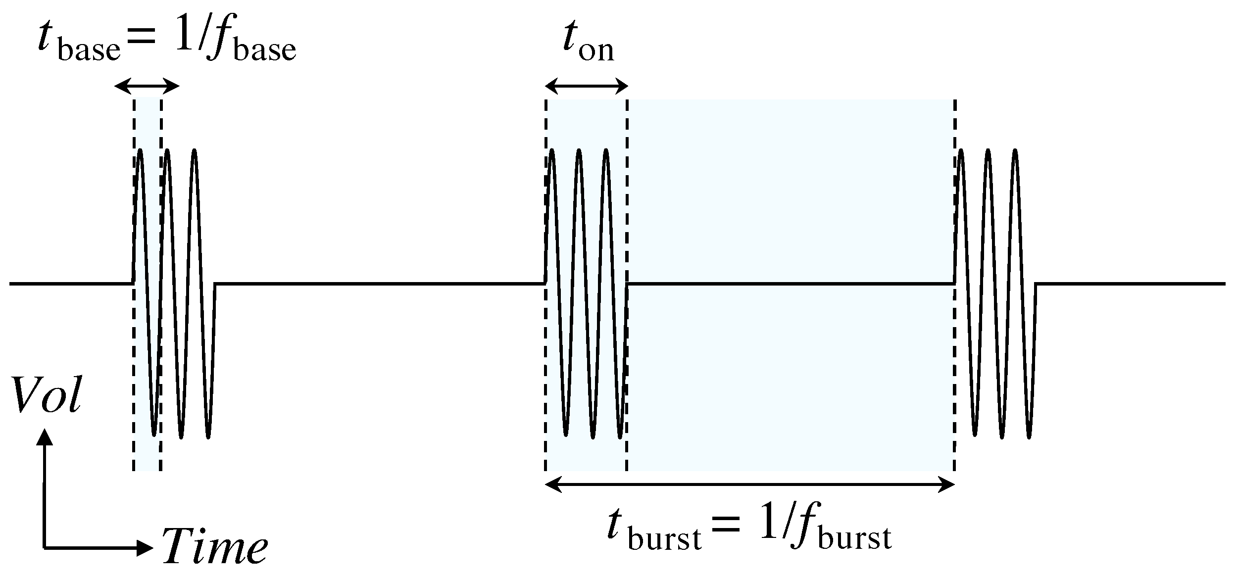
2. PA Drive Methods and Computational Cases

The plasma actuator is installed at 5% chord length from the leading edge. This position is close to the separation point of the flow at $\mathsf{\alpha }$ = 12 and is effective for flow separation control [8]. Two PA drive methods are considered in the present study.

The continuous actuation is a standard drive method of PA. The AC voltage, which is based on a base frequency $f_{\mathrm{base}}$ is continuously applied to the PA. The burst actuation is the other method of driving PA. The AC voltage modulated with the duty cycle is applied to PA during the burst actuation. Figure 2 shows a schematic diagram of the AC voltage waveform for the burst actuation. Parameters of the waveform are defined as in Equation (1). $f_{\mathrm{base}}$ is a base frequency of the AC voltage waveform. $t_{\mathrm{on}}$ and $t_{\mathrm{burst}}$ are the driving time and burst period, respectively. $f_{\mathrm{burst}}$ denotes the burst frequency. $F^{+}$, $F_{\mathrm{base}}$, and $BR$ are non-dimensional $f_{\mathrm{burst}}$, non-dimensional $f_{\mathrm{base}}$, and burst ratio, respectively. Previous studies [30,33] have shown that the burst actuation controls flow separations more efficiently than the continuous actuation at low Reynolds numbers ($Re\simeq {10}^4$–${10}^5$) at post-stall angles of attack.

The studies show that the burst actuation with $F^{+}=6$ and $BR=0.1$, which promotes a turbulent transition, is effective for suppressing a flow separation at $\alpha =12$. In the present study, the burst actuation with those burst parameters was employed to confirm a flow control authority of PA at pre-stall angles of attack.

Hereafter, we call a computational case of the continuous drive a “Continuous” case and the burst drive a “Burst” case. In both cases, $F_{\mathrm{base}}$ is set to 60 according to the previous experimental and computational studies [8,31]. In addition to the computational cases with PA, Flows without PA are considered, called “PA-OFF” cases, as baseline flows. Four angles of attack $\alpha =$ 4, 6, 8, and 10 are considered. Therefore, the total number of computational cases is 12. In addition, each case at $\alpha =12$ is used to discuss the difference in the phenomena at pre-stall and post-stall angles.

$$\begin{array}{c}\hfill F^{+}=\frac{f_{\mathrm{burst}}c}{U_{\infty }},F_{\mathrm{base}}=\frac{f_{\mathrm{base}}c}{U_{\infty }},BR=\frac{t_{\mathrm{on}}}{t_{\mathrm{burst}}}.\end{array}$$

(1)

3. Computational Approach

3.1. Governing Equations

Three-dimensional compressible Navier–Stokes equations with the source term added were solved in the present study. The equations are non-dimensionalized by the free-stream density, free-stream velocity, and chord length of the airfoil and are represented as follows:

$$\begin{array}{ccc}\hfill \frac{\partial \rho }{\partial t}+\frac{\partial \rho u_j}{\partial x_j}& =& 0,\hfill \end{array}$$

(2)

$$\begin{array}{ccc}\hfill \frac{\partial \rho u_i}{\partial t}+\frac{\partial \left(\rho u_i{u}_j+p{\delta }_{ij}\right)}{\partial x_j}& =& \frac{1}{Re}\frac{\partial {\tau }_{ij}}{\partial x_j}+D_{\mathrm{c}}{S}_i,\hfill \end{array}$$

(3)

$$\begin{array}{ccc}\hfill \frac{\partial e}{\partial t}+\frac{\partial \left(\left(e+p\right)u_j\right)}{\partial x_j}& =& \frac{1}{Re}\frac{\partial u_k{\tau }_{jk}}{\partial x_j}-\frac{1}{\left(\gamma -1\right)PrRe{M}_{\infty }^2}\frac{\partial q_j}{\partial x_j}+D_{\mathrm{c}}{S}_j{u}_j,\hfill \end{array}$$

(4)

where $\rho$, $u_i$, p, e, $q_i$, $x_i$, t, and ${\tau }_{ij}$ denote the non-dimensional forms of the density, velocity vector, pressure, energy per unit volume, heat flux vector, position vector, time, and stress tensor, respectively. ${\delta }_{ij}$ is the Kronecker delta. Equations (2)–(4) follow Einstein notation. The subscript i is a free index, and j and k are dummy indices. The indices take the value 1, 2, or 3. $Re$, $M_{\infty }$, and $Pr$ denote the Reynolds number, free-stream Mach number, and Prandtl number, respectively. They are defined as follows:

$$\begin{array}{c}\hfill Re=\frac{{\rho }_{\infty }{U}_{\infty }c}{{\mu }_{\infty }},M_{\infty }=\frac{U_{\infty }}{a_{\infty }},Pr=\frac{{\mu }_{\infty }{c}_{\mathrm{p}}}{{\kappa }_{\infty }},\end{array}$$

(5)

where ${\rho }_{\infty }$, $U_{\infty }$, c, ${\mu }_{\infty }$, $a_{\infty }$, $c_{\mathrm{p}}$, and ${\kappa }_{\infty }$ denote the density, velocity, chord length, viscosity, sound speed, constant pressure specific heat, and heat conduction coefficient, respectively. Here, a quantity with subscript ∞ denotes the quantity in the free-stream condition. The viscosity is calculated using Sutherland’s law. $D_{\mathrm{c}}{S}_i$ and $D_{\mathrm{c}}{S}_j{u}_j$ in Equations (3) and (4) correspond to the body force and power added to the unit volume by PA, respectively. Hereinafter, x, y, z, u, v, and w are used to represent the position and flow velocity of $x_1$, $x_2$, $x_3$, $u_1$, $u_2$, and $u_3$, respectively, for ease of discussion. In the present study, the free-stream Mach number is set to 0.2, which reduces the computational time. The compressibility of the fluid is almost negligible although the Mach numbers in the present study and previous experimental studies [29,30] are different.

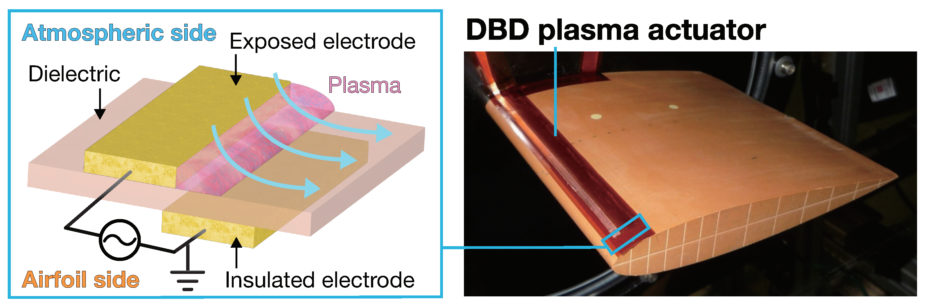
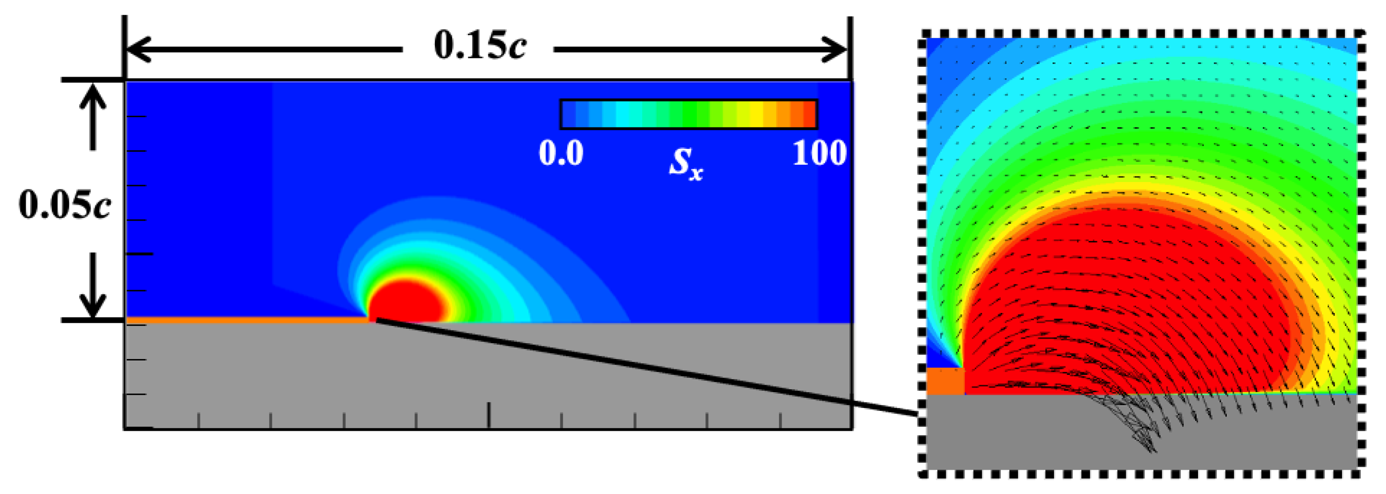
3.2. Plasma Actuator Modeling

The body force term for PA was modeled with $D_{\mathrm{c}}{S}_i$ and $D_{\mathrm{c}}{u}_k{S}_k$ in the Navier–Stokes equations, as in Equations (3) and (4). The Suzen–Huang model [34] is utilized to obtain $S_i$. The non-dimensional body force vector $S_i$ is represented as follows:

$$S_i={\rho }_{\mathrm{c}}\left(-{\displaystyle \frac{\partial \varphi }{\partial x_i}}\right)f{\left(t\right)}^2,$$

(6)

where $f\left(t\right)$ is the waveform function of the input voltage, ${\rho }_{\mathrm{c}}$ is the net charge density, and $\varphi$ is the electric potential. The following equations are solved to obtain ${\rho }_{\mathrm{c}}$ and $\varphi$:

$$\begin{array}{ccc}\hfill {\displaystyle \frac{\partial }{\partial x_j}}\left({\epsilon }_{\mathrm{r}}{\displaystyle \frac{\partial \varphi }{\partial x_j}}\right)& =& 0,\hfill \end{array}$$

(7)

$$\begin{array}{ccc}\hfill {\displaystyle \frac{\partial }{\partial x_j}}\left({\epsilon }_{\mathrm{r}}{\displaystyle \frac{\partial {\rho }_{\mathrm{c}}}{\partial x_j}}\right)& =& {\displaystyle \frac{{\rho }_c}{{\lambda }_{\mathrm{d}}^2}},\hfill \end{array}$$

(8)

where ${\epsilon }_{\mathrm{r}}$ is the relative permittivity of the medium, and ${\lambda }_{\mathrm{d}}$ is the Debye length.

The following plasma actuator was considered in the present study: The exposed electrode was 2 mm wide, and the insulated electrode was $8.75$ mm wide. The electrodes were $0.1$ mm thick and separated by a $0.1$ mm thick dielectric. The streamwise spacing of electrodes was $0.5$ mm. The dielectric was Kapton, and ${\epsilon }_{\mathrm{r}}$ was 2.7. In the air, ${\epsilon }_{\mathrm{r}}$ was 1.0. For ${\lambda }_{\mathrm{d}}$, the same 1 mm as in the previous study was used [34]. These length parameters were non-dimensionalized by the reference length $c=0.1$ m. Equations (7) and (8) were solved by the successive over-relaxation (SOR) method using a $1201\times 801$ two-dimensional mesh. Boundary conditions for Equation (7) are given as follows:

on outer boundaries,	$\partial \varphi /\partial n_i=0$,
on exposed electrode,	$\varphi =1.0$,
on insulated electrode,	$\varphi =0$,

where $n_i$ is the unit normal vector. The boundary conditions for Equation (8) are given as:

on outer boundaries and in dielectric,	${\rho }_{\mathrm{c}}=0$,
on the surface of dielectric above the insulated electrode,	${\rho }_{\mathrm{c}}=G\left(x^{\prime }\right)$,
on the other surface of PA,	$\partial {\rho }_{\mathrm{c}}/\partial n_i=0$.

$G\left(x^{\prime }\right)$ is given by a half Gaussian distribution as follows:

$$G\left(x^{\prime }\right)=\exp \left(-{\displaystyle \frac{x^{\prime 2}}{2{\delta }^2}}\right),$$

(9)

where $x^{\prime }$ is the chordwise length measured from the edge of the insulated electrode, and $\delta$ was $0.3l_{\mathrm{e}}$ in the present study. $l_{\mathrm{e}}$ is the insulated electrode length. In the present study, the input voltage is a standard alternating current. Therefore, the waveform $f\left(t\right)$ is the sinusoidal wave:

$$f\left(t\right)=\sin \left(2\pi F_{\mathrm{base}}t\right).$$

(10)

Figure 3 shows the distribution of the body force magnitude in the x direction ($S_x$) when $f\left(t\right)=1$. The body force vectors are also shown in an enlarged view near PA. The length of the model region is $0.15c$ in the chordwise direction and $0.05c$ in the wall-normal direction. The body force in the spanwise direction was not implemented so that no disturbance in the spanwise direction could be included in the plasma actuation of the present simulations. The magnitude of the body force was determined by the non-dimensional input voltage parameter, $D_c$, which is defined as follows:

$$\begin{array}{c}\hfill D_{\mathrm{c}}={\displaystyle \frac{{\rho }_{\mathrm{c},\max }{\varphi }_{\max }}{{\rho }_{\infty }{U}_{\infty }^2}},\end{array}$$

(11)

where ${\rho }_{\mathrm{c},\max }$ and ${\varphi }_{\max }$ are the maximum values of ${\rho }_{\mathrm{c}}$ and $\varphi$. In the present study, $D_{\mathrm{c}}=0.04$ was used. The maximum induced velocity produced by continuous actuation with $D_{\mathrm{c}}=0.04$ in quiescent air reaches approximately $3.4$ m/s if the reference velocity is $U_{\infty }=10$ m/s [32]. This value is equivalent to the induced velocity produced by PA with a peak-to-peak applied voltage of 9 kV [31]. In the present body force model, the fluctuation is modeled by the square of the sinusoidal function. The direction of the body force produced by this fluctuation does not change within a single AC cycle, and even if the phase of the AC voltage changes, the body force in the opposite direction is not generated. This characteristic is similar to that of the “push-push type” model suggested by Font et al. [35]. $F_{\mathrm{base}}$ was set to 60, which corresponds to the frequency used in previous experiments [29,30]. Although the present model is simple, we validated it by comparing the LES results and the experimental results [23]. In addition, we also confirmed that the LES results using this model were not significantly different from those using a high-fidelity model [36]. Note that the flow induced by the plasma actuator in quiescent air conditions is considered to be unchanged for freestream velocities below 100 m/s [37]. In the present study, the freestream velocity is assumed to be 10 m/s. Therefore, the model equations were not solved concurrently with Navier–Stokes equations but in advance.

The obtained body force is mapped to the computational grid for LES after rotating around the downstream edge of the exposed electrode to match the tangential direction of the airfoil surface.

3.3. Computational Method

We employ the flow solver LANS3D, which has been developed and verified to achieve high-fidelity simulations [38,39,40]. Generalized curvilinear coordinates ($\xi ,\eta ,\zeta$) were adopted to solve the governing equations. The spatial derivatives of the convective and viscous terms, metrics, and Jacobians were evaluated using a sixth-order compact difference scheme [41]. At the first and second points off the wall boundary, a second-order explicit difference scheme was adopted. Tenth-order low-pass filtering [41,42] was used with a filtering coefficient of 0.495. A backward second-order difference formula was used for time integration, and five sub-iterations [43] were adopted to ensure time accuracy. For time integration, the lower-upper symmetric alternating direction implicit and symmetric Gauss–Seidel (ADI-SGS) [44] methods were used. The time step size nondimensionalized by the free-stream velocity and the chord length was $4\times {10}^{-5}$. The maximum Courant number was approximately 2.0. The nondimensional time step based on the wall units was lower than 0.025 at the attached turbulent boundary layer. Choi and Moin [45] indicated that a time step of less than 0.4 is sufficient for the LES on a turbulent boundary layer. In the present study, wall-resolved LESs were conducted. The LES using the compact difference scheme with the high-order low-pass filter is well-validated and shows comparable results with standard LESs with explicit sub-grid-scale models when the computational grid resolution is fine enough [46,47,48]. The high-order low-pass filter adds numerical viscosity to computations at the only coarse grid region and implicitly acts as sub-grid scale models. Thus, the explicit sub-grid scale models were not used in the present study to avoid unpreferable turbulence decay. Utilized grid resolutions in the present study are explained in Section 3.4.

All variables were extrapolated from the point inside the outflow boundary into the point at the boundary. At the outflow boundary, all variables were extrapolated from the grid points next to the boundary into the grid points at the boundary, and the static pressure was fixed as the free stream value. At the wall boundary, adiabatic and no-slip conditions were applied. For the boundaries in the spanwise direction, a periodic boundary condition was adopted. At the inflow boundary, a uniform free stream condition without disturbance was employed.

All LESs were performed using the JAXA Supercomputer System Generation 2 and 3 (JSS2 and JSS3) at the Japan Aerospace Exploration Agency. Approximately 80 nodes (2560 cores) were used for each case.

The computations were conducted until the aerodynamic coefficients became quasi-steady before obtaining the time-averaged flow field and aerodynamic coefficients. The computational time in nondimensional time before obtaining the data was longer than 30. The data obtaining duration was five in nondimensional time.

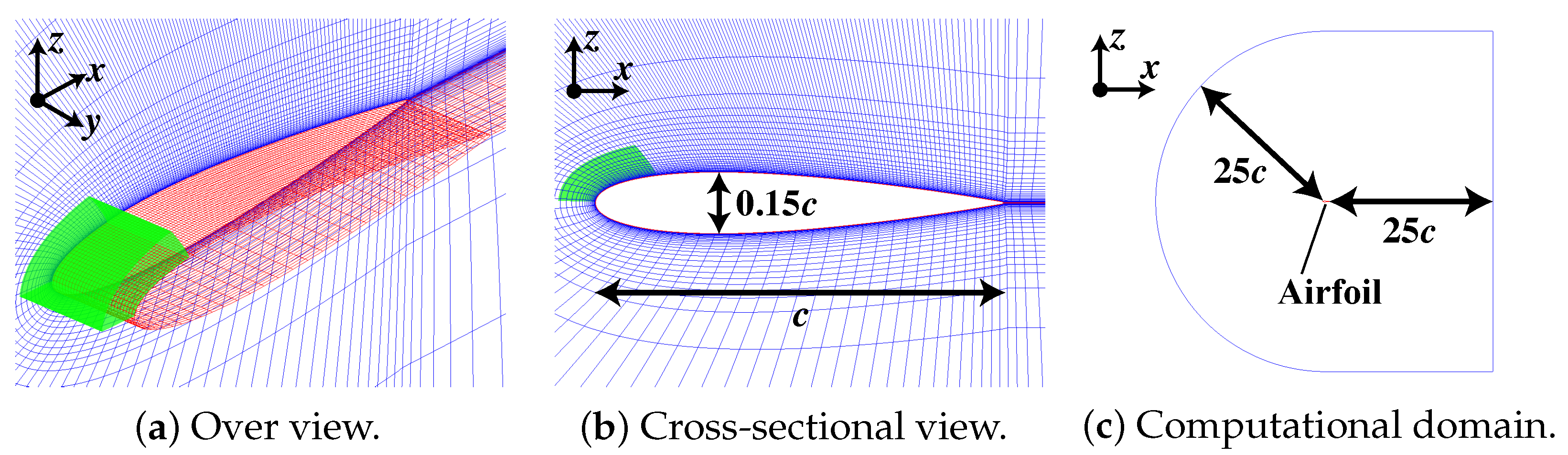
3.4. Computational Grid

The computational grids and the computational domain with a schematic diagram of the inflow are shown in Figure 4. The zonal method [49] using two computational grids with different resolutions were employed to treat small fluid fluctuations induced by PA in the present LES. The computational grids consist of a C-type grid around the airfoil (zone1: blue and red) and a fine grid around PA (zone 2: green). The body force of the Suzen–Huang model was obtained in advance and mapped to zone 2. Equations (2)–(4) were solved for zones 1 and 2, and physical values were exchanged with each other at every time step.

The distance from the airfoil surface to the outer boundary was $25c$, and the width of the span-wise computational domain was $0.2c$. The grid points of zone 1 and zone 2 were approximately $1.8\times {10}^7$ and $2.0\times {10}^6$, respectively, as shown in

Table 1. Number of computational grid points.

	$\mathit{\xi }$	$\mathit{\eta }$	$\mathit{\zeta }$	Total Point
Zone 1	759	134	179	18,205,374
Zone 2	149	134	111	2,216,226

. The minimum grid spacing in the wall-normal direction was $0.00012c$. The maximum grid sizes based on the wall unit were $(\Delta {\xi }^{+},\Delta {\eta }^{+},\Delta {\zeta }^{+})\lesssim (8,9,1)$ at the attached turbulent boundary layer region. The present grid resolution and the computational methods were validated in the previous study [23].

4. Results and Discussion

4.1. Validation

Here, the present LESs are validated by comparing them with the experimental results. The experimental data were acquired using the same facility at the Institute of Space and Astronautical Science, Japan Aerospace Exploration Agency (JAXA), utilized in the previous study [30]. The test section size of the wind tunnel was 100 mm in width, 400 mm in height, and 700 mm in length. The turbulence intensity at the center of the tunnel was verified to be approximately 0.08% at a freestream velocity of 6.6 m/s. A two-dimensional NACA0015 wing model with a chord length of 100 mm and a span length of 100 mm was used. The model surface had a total of 29 pressure ports, and the time-averaged pressure measurements were conducted, but the pressure around $x/c=0.05$ could not be measured due to the PA installation on the airfoil surface. The freestream velocity was set to 10 m/s, corresponding to the Reynolds number of approximately 63,000, based on the chord length and the freestream velocity, which is the same as the present LES. The applied voltage of PA was 3.5 kV${}_{\mathrm{pp}}$ (peak-to-peak voltage). The details may be found in the literature [30]. It should be noted that the experimental results include the effect of the wind tunnel’s side walls and the freestream disturbance.

Figure 5 compares pressure coefficient ($C_{\mathrm{p}}$) distributions at $\alpha =6,8,$ and 10 obtained by the LESs and experiments. The shape of the NACA0015 airfoil is shown in gray on the background.

Table 2. Mean absolute errors (MAE) between the $C_{\mathrm{p}}$ distributions obtained by the LESs and the experiments.

	$\mathit{\alpha }$ [deg]
	6	8	10
PA-OFF	0.076	0.078	0.064
Continuous	0.115	0.098	0.097
Burst	0.094	0.059	0.078

shows mean absolute errors (MAE) between the $C_{\mathrm{p}}$ distributions obtained by the LESs and the experiments.

In the PA-OFF case at $\alpha =10$ (Figure 5a) and the Burst cases (Figure 5c), the LES results show quantitative agreement with the experimental results at all angles of attack. The MAE values are relatively low in these case. On the other hand, in the PA-OFF case at $\alpha =6$ and 8 and the Continuous case, the LESs overestimate the plateau region of $C_{\mathrm{p}}$ distribution. This discrepancy between the LESs and experiments is probably because of a tripping effect of the PA electrodes on the airfoil surface and a freestream disturbance [30]. These disturbances would make the Continuous case’s flow of experiments close to that of the Burst case. The parameter $D_{\mathrm{c}}$ uncertainty, which is set to match the maximum value of the PA-inducing velocity, also might affect the computational results. Although a discussion of the Continuous case needs to be conducted carefully; we consider that the LES results are reliable enough to discuss the effectiveness of PA because the LESs can predict the quantitative agreement of the Burst cases and the qualitative tendency that the plateau region in each case becomes smaller as the angle of attack increases. In addition, the computational method and the PA model used in the present study have been validated even at the angle of attack after stall [8,23].

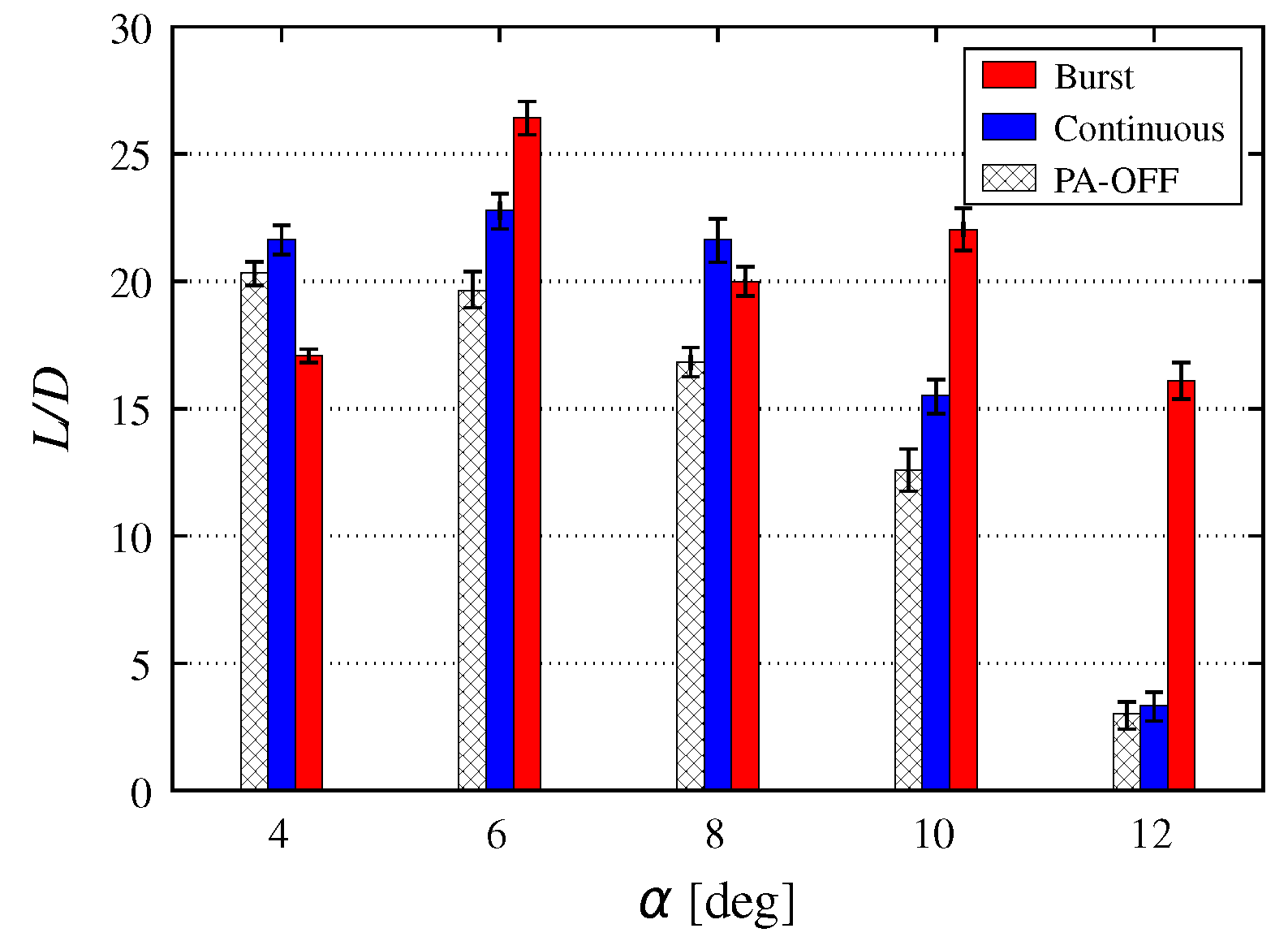
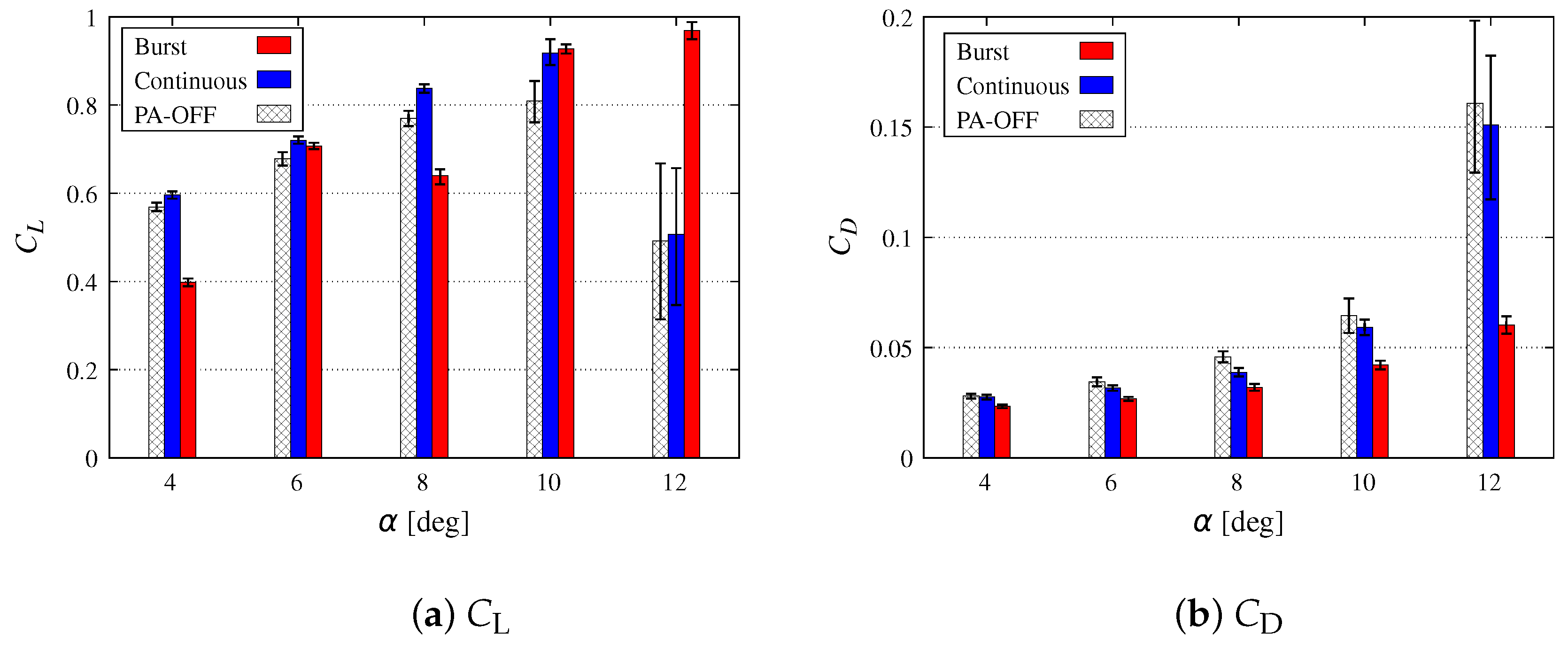
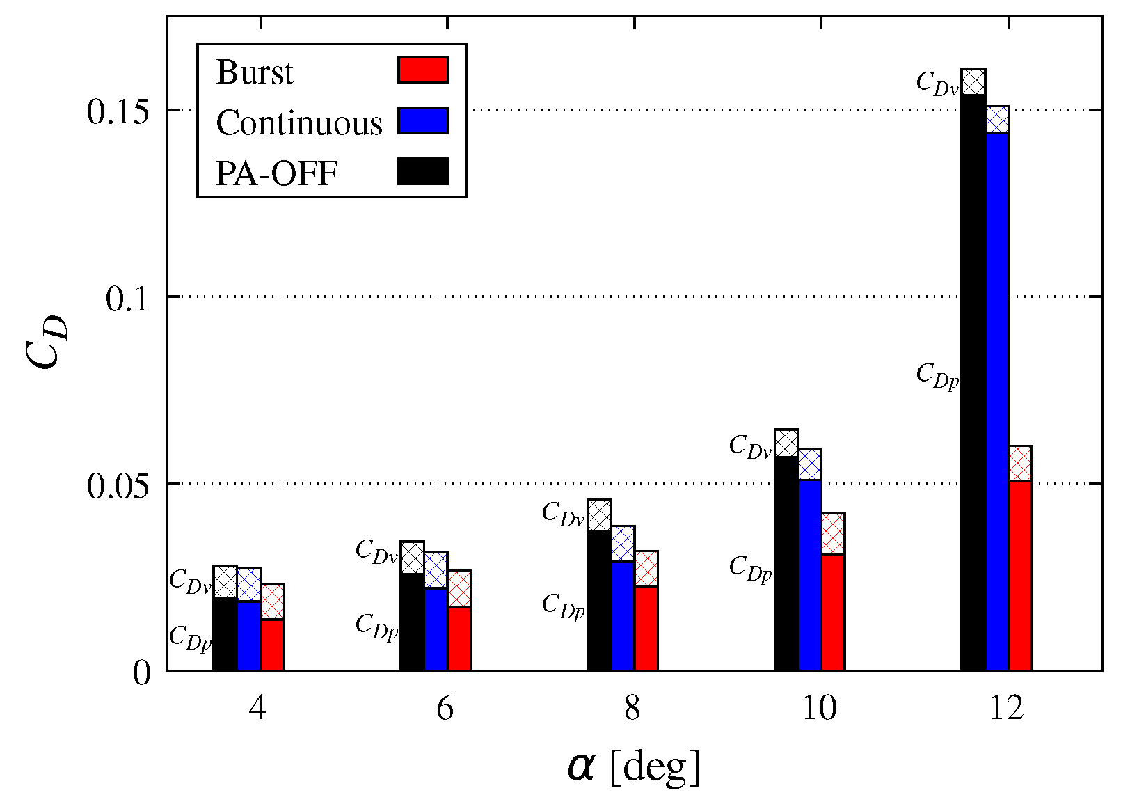
4.2. Aerodynamic Characteristics

Figure 6 shows the average value of the lift-to-drag ratio ($L/D$) with the minimum and maximum values in each case. The Continuous and Burst cases show the $L/D$ value superior to the PA-OFF cases except for the Burst case at $\alpha =4$. This result indicates that the flow control using PA helps the improvement in the aerodynamic characteristics even at lower angles of attack than the stall angle.

Figure 7 shows the lift coefficient ($C_{\mathrm{L}}$) and drag coefficient ($C_{\mathrm{D}}$) in each case. The $C_{\mathrm{L}}$ of the Continuous case was higher than the PA-OFF case in all cases, while $C_{\mathrm{L}}$ of the Burst case at $\alpha =4$ and 8 was lower than PA-OFF. The $C_{\mathrm{D}}$ values of Continuous and Burst cases were more stable than the PA-OFF case at any angle of attack and control method, and the fluctuation was slight. At the post-stall angles of attack, $L/D$ improved by a $C_{\mathrm{L}}$ increase and a $C_{\mathrm{D}}$ decrease [23]. However, at $\alpha =8$, which is a pre-stall angle of attack, $C_{\mathrm{L}}$ of the Burst case was lower than the PA-OFF case. On the other hand, the $C_{\mathrm{D}}$ of the Burst case was lower than the PA-OFF case, and as a result, $L/D$ was higher than the PA-OFF case. In other words, at the pre-stall angle of attack, the reduction of $C_{\mathrm{D}}$ contributes more to the improvement of $L/D$ than the improvement of $C_{\mathrm{L}}$.

Figure 8 shows the breakdown of $C_{\mathrm{D}}$: viscous drag ($C_{{\mathrm{D}}_{\mathrm{v}}}$) and pressure drag ($C_{{\mathrm{D}}_{\mathrm{p}}}$) in each case. Although there was no significant change in $C_{{\mathrm{D}}_{\mathrm{v}}}$ by using PA, $C_{{\mathrm{D}}_{\mathrm{p}}}$ decreased in both pre-stall and post-stall angles. In particular, the reduction in $C_{{\mathrm{D}}_{\mathrm{p}}}$ was more remarkable in the Burst cases than in the Continuous cases. The $C_{{\mathrm{D}}_{\mathrm{p}}}$ reduction effect of the Burst cases is discussed in detail in the following section (Section 4.3).

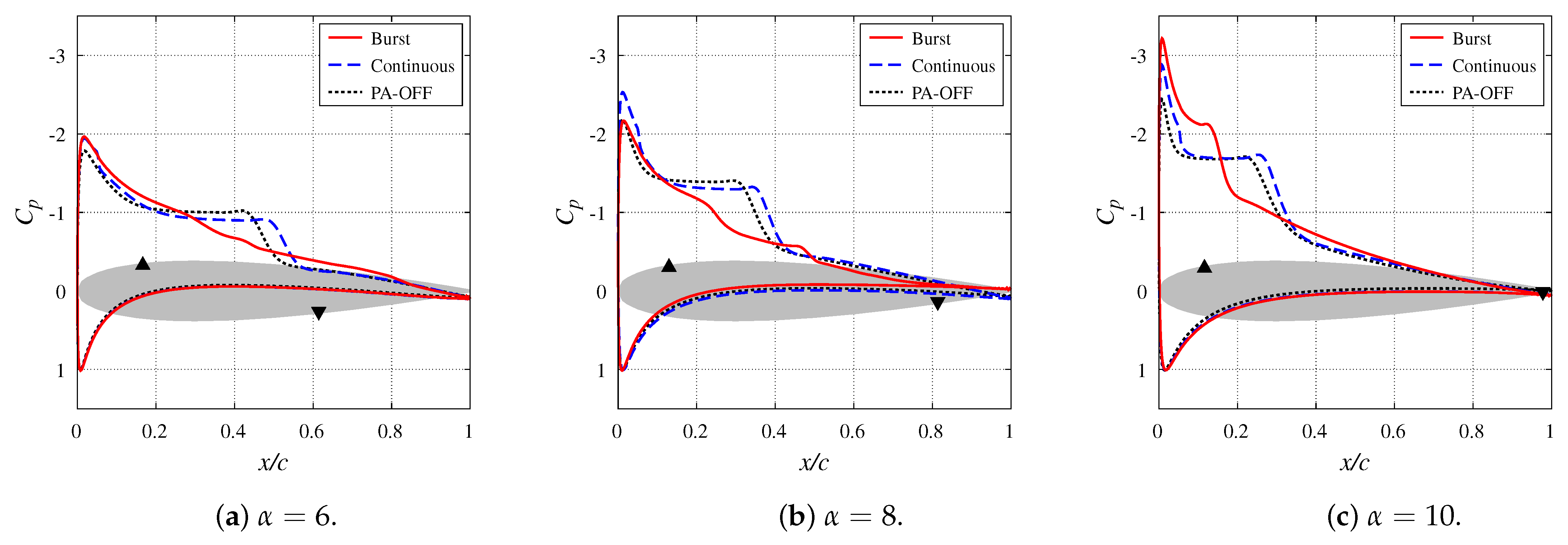
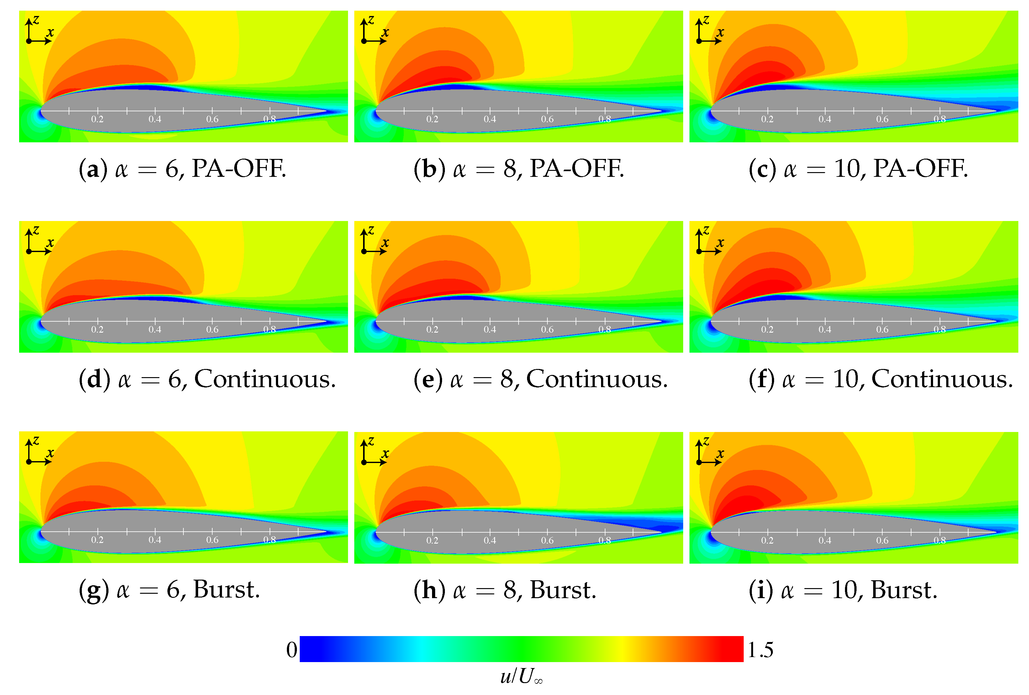
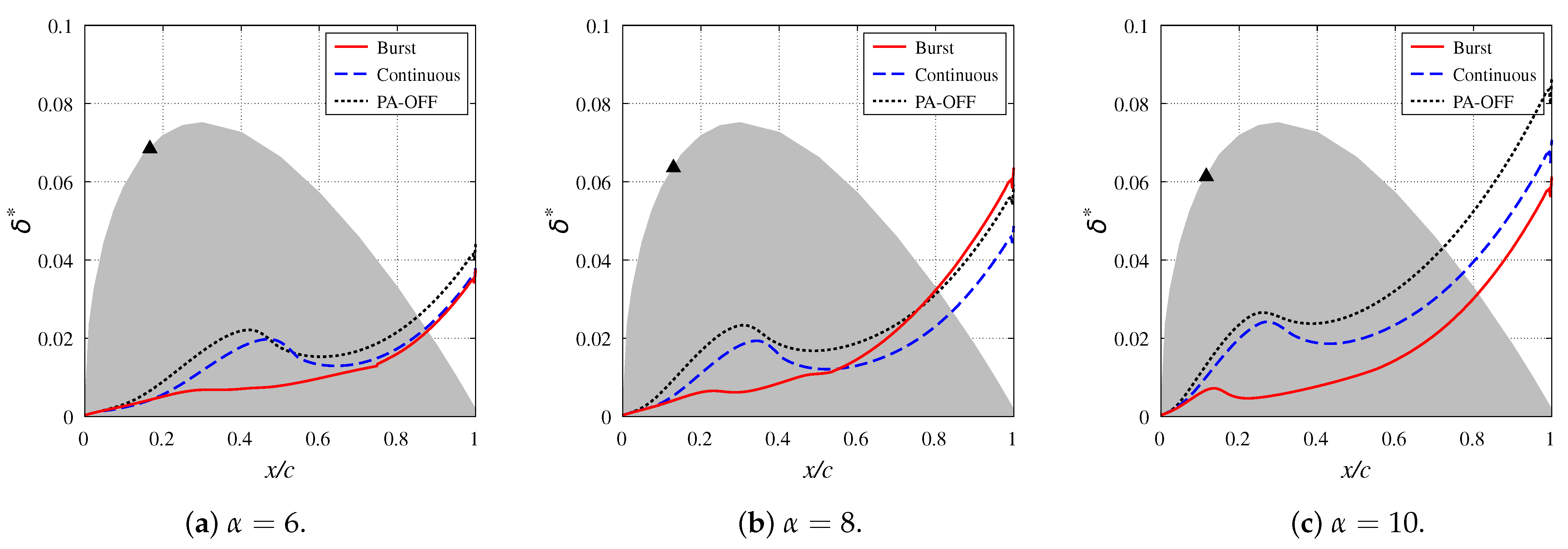
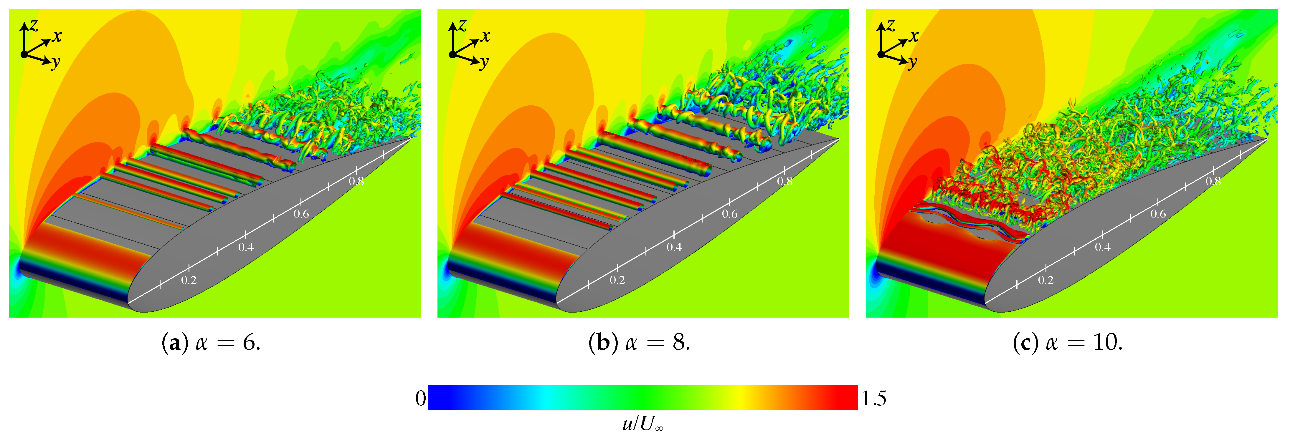
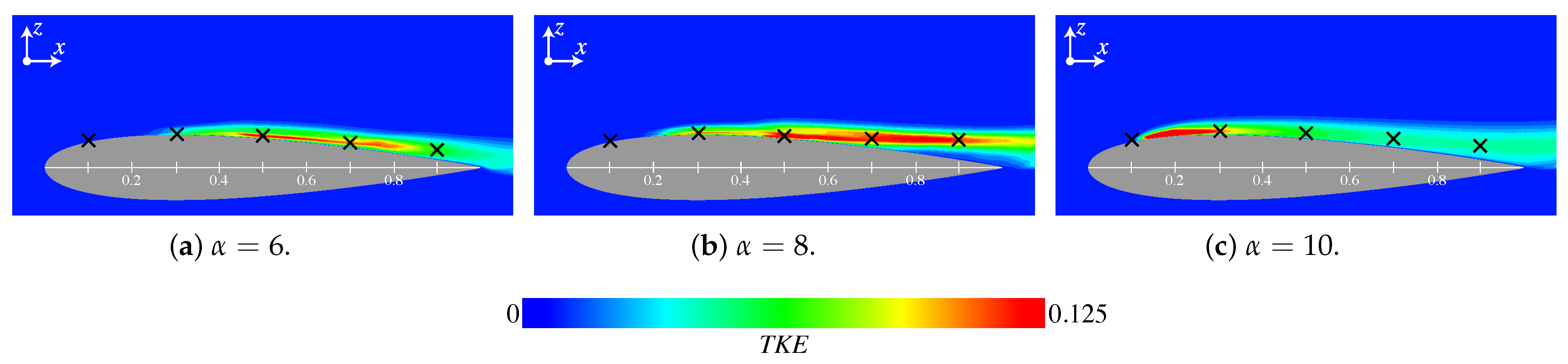
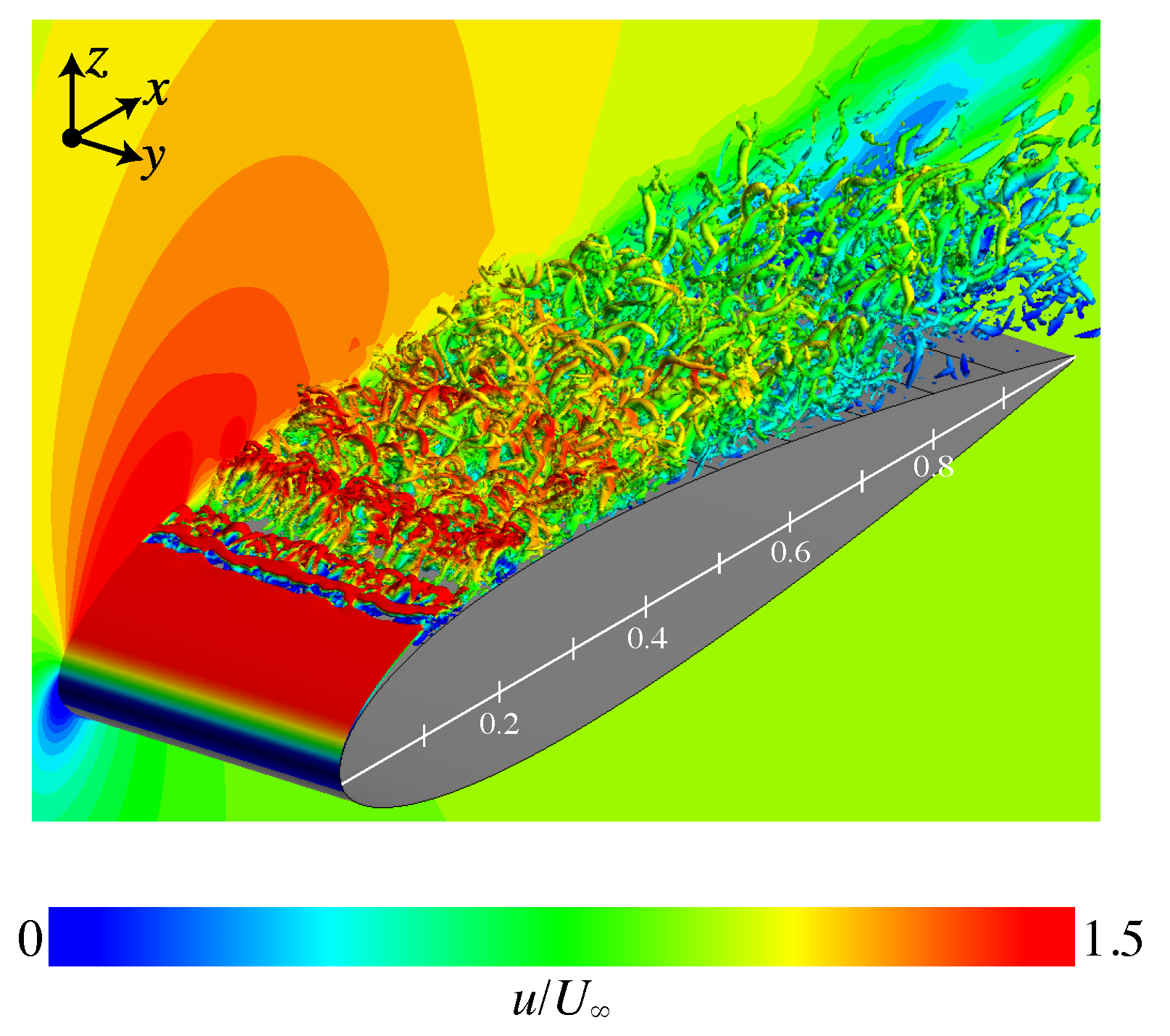
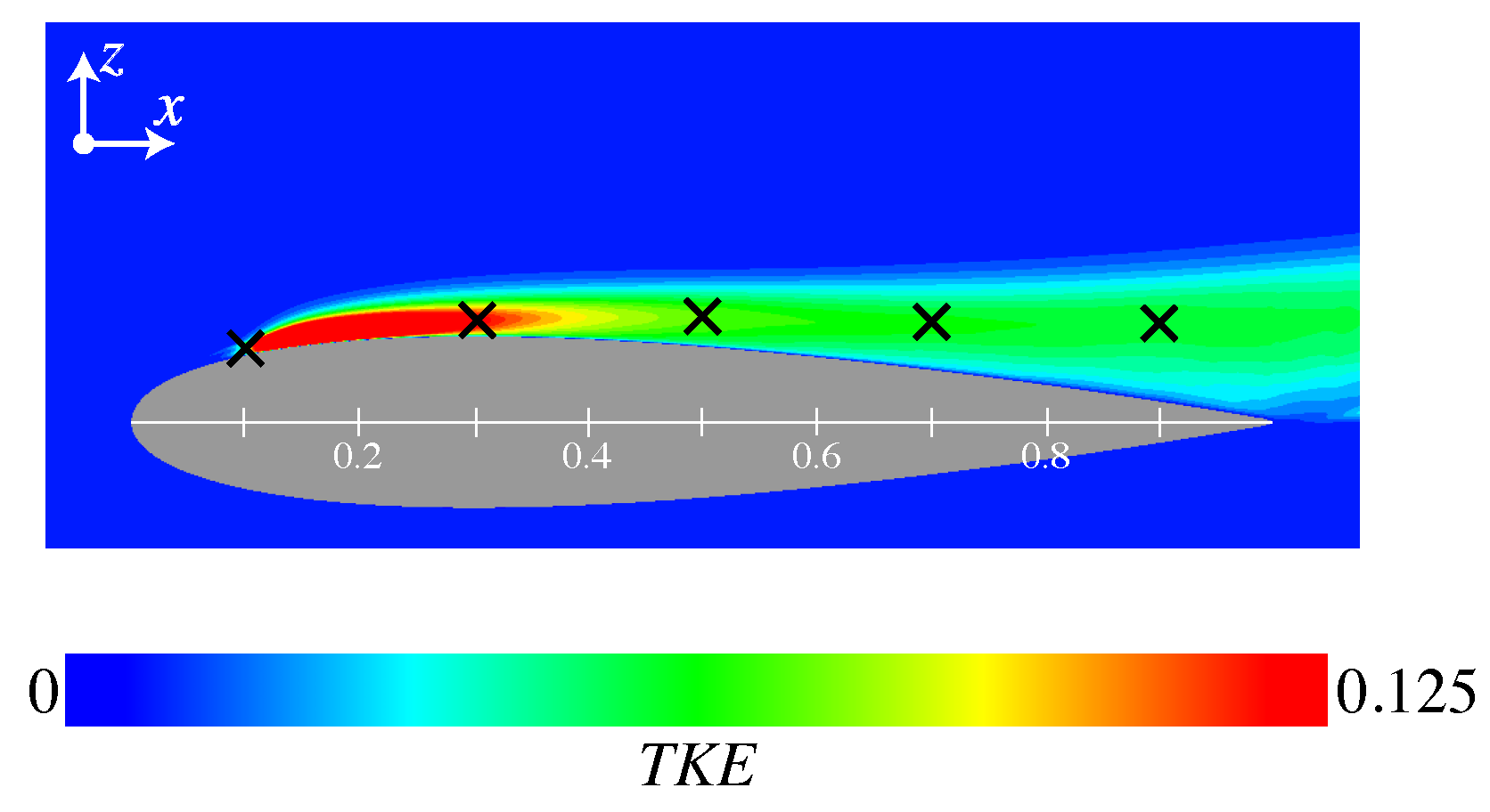
4.3. Averaged Flow Feature

In this section, we discuss what flow changes with the PA control cause an aerodynamic characteristic change. In the following discussion, the results at $\alpha =4$ are omitted because their overall tendency is similar to that at $\alpha =6$, and arguments will be made with the results at $\alpha =6,8,$ and 10.

Figure 9 shows the pressure coefficient ($C_{\mathrm{p}}$) distribution around the airfoil obtained in each case. The shape of the NACA0015 airfoil is drawn in gray on the background. The black up- and down-pointing triangle symbols indicate the highest and lowest airfoil surface positions at each angle of attack, respectively. The characteristic changes in the $C_{\mathrm{p}}$ distribution with the PA control are mainly observed on the airfoil’s upper surface. In the Continuous cases, the $C_{\mathrm{p}}$ value at the suction peak near the leading edge lowered, and the plateau region moved toward the trailing edge and slightly shrunk. In the Burst cases, the $C_{\mathrm{p}}$ plateau region was significantly reduced, and the $C_{\mathrm{p}}$ value at the suction peak became low at $\alpha =6$ and 10. The local variation of $C_{\mathrm{p}}$ seen at $0.2\lesssim x/c\lesssim 0.5$ in the Burst cases at $\alpha =6$ and 8 was due to the merging of the two-dimensional vortex structures. The details are discussed in Section 4.4. Additionally, at $\alpha =8$, the pressure on the underside of the airfoil was slightly lower than that of the PA-OFF and Continuous cases.

We discuss the $C_{\mathrm{p}}$ distribution in more detail from the perspective of reducing $C_{{\mathrm{D}}_{\mathrm{p}}}$. Since the force due to the surface pressure acts perpendicularly to the airfoil surface, the force contribution direction (thrust or drag) depends on the orientation of the airfoil surface. When there is no inflection point on the suction side, such as the NACA0015 airfoil, the surface pressure at the front half region from the highest point of the airfoil contributes to thrust, while the surface pressure at the back half part from the highest point contributes to drag increase. In Figure 9, since the suction peak exists upstream from the highest point in each case, the lower the pressure at the peak position, the more significant the contribution to thrust and the lower $C_{{\mathrm{D}}_{\mathrm{p}}}$. On the contrary, in the PA-OFF case shown in Figure 9, most of the plateau region caused by the separation bubbles exists downstream from the highest point; thus, the negative pressure contributes to the drag.

Figure 10 shows the distribution of the skin-friction coefficient ($C_{\mathrm{f}}$) on the airfoil’s upper surface in each case. In the PA-OFF case at $\alpha =6$, $C_{\mathrm{f}}$ is negative in the range of $0.1\lesssim x/c\lesssim 0.5$, indicating that the flow is separated and forms separation bubbles. The negative $C_{\mathrm{f}}$ region coincides with the plateau region in Figure 9a. In the Continuous cases in Figure 9, the pressure of the suction peak is reduced at any angle of attack. On the other hand, as shown in Figure 10, the plateau region in Figure 9 is moved to the trailing edge side due to the movement of the separation bubble position (the area where $C_{\mathrm{f}}$ is negative) to the downstream. The movement of this plateau region to the downstream contributes to the $C_{{\mathrm{D}}_{\mathrm{p}}}$ increase. However, since the contribution of the $C_{{\mathrm{D}}_{\mathrm{p}}}$ decrease because the pressure decrease in the suction peak is larger and $C_{{\mathrm{D}}_{\mathrm{p}}}$ slightly decreases at any angle of attack, as shown in Figure 8. In the Burst cases, the suction peak value of $C_{\mathrm{p}}$ near the leading edge is lower than the other cases at $\alpha =6$ and 10 (Figure 9a,c). In addition, the plateau region is reduced at all angles of attack, and therefore, $C_{{\mathrm{D}}_{\mathrm{p}}}$ value becomes lower than the Continuous cases.

The relationship between the flow field and the pressure distribution on the airfoil surface is discussed in more detail. Figure 11 shows time- and spanwise-averaged flows colored with the chordwise velocity normalized by the freestream velocity (u/$U_{\infty }$) for each case, and Figure 12 shows the displacement thickness (${\delta }^{*}$) on the airfoil’s upper surface. Figure 11 and Figure 12 are helpful in understanding the separation bubble size in the wall-normal direction of the airfoil. The displacement thickness is nondimensionalized by the chord length. The NACA0015 airfoil is shown in the background to the same scale as the displacement thickness. In all cases, the flow separates from around $x/c\simeq 0.1$, forming a separation bubble, although it is difficult to see in the Burst cases.

The flow on the airfoil’s upper surface (suction side) generally accelerates due to the flow bending at the leading edge of the airfoil (the red region in Figure 11), creating the suction peak, as seen in Figure 9. In the present flow fields, the shape of the separation bubble existing in this acceleration region changes due to the PA control; thus, the value of the suction peak also changes in each case. The pressure distribution in the presence of the separated region on the airfoil surface can be predicted by assuming that the airfoil thickness increases as much as the thickness of the separated region. The smaller the displacement thickness, the lower the effect of the boundary layer and separated area, and the flow becomes closer to the potential flow of the NACA0015 airfoil.

In Figure 12, the displacement thicknesses of the Continuous and Burst cases are smaller than that of the PA-OFF case in the region of $0.1\lesssim x/c\lesssim 0.4$ at any angle of attack. When the flow bends, the pressure inner side of the curved flow becomes lower as the radius of curvature becomes smaller. Therefore, in the Continuous and Burst cases with the thin displacement thickness, the radius of curvature of the flow near the leading edge of the airfoil is smaller than in the PA-OFF case, and the pressure is lower. However, in Figure 9b, the suction peak value of the burst case at $\alpha =8$ is almost the same as that of the PA-OFF case. The exceptional suction value of the burst case at $\alpha =8$ may be caused by the flow separation near the trailing edge on the suction side. At $x/c\simeq 0.9$ in Figure 10b, $C_{\mathrm{f}}$ is almost zero, and in Figure 11h, the low-speed region is larger near the trailing edge than in the other cases. Due to this trailing edge separation, in Figure 10b, the displacement thickness of the Burst case near the trailing edge ($0.8\lesssim x/c\lesssim 1$) becomes the thickest, and the radius of curvature on the airfoil’s upper surface increases, resulting in weakening the acceleration of the flow near the leading edge and affecting the value of the suction peak.

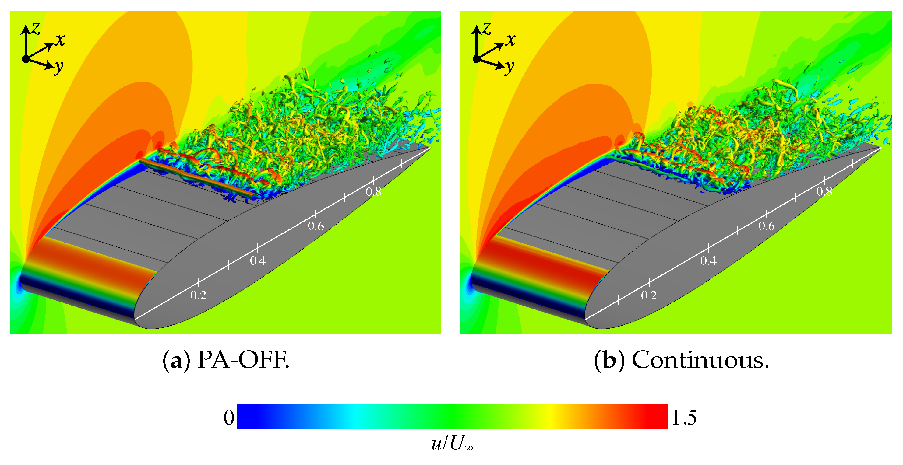
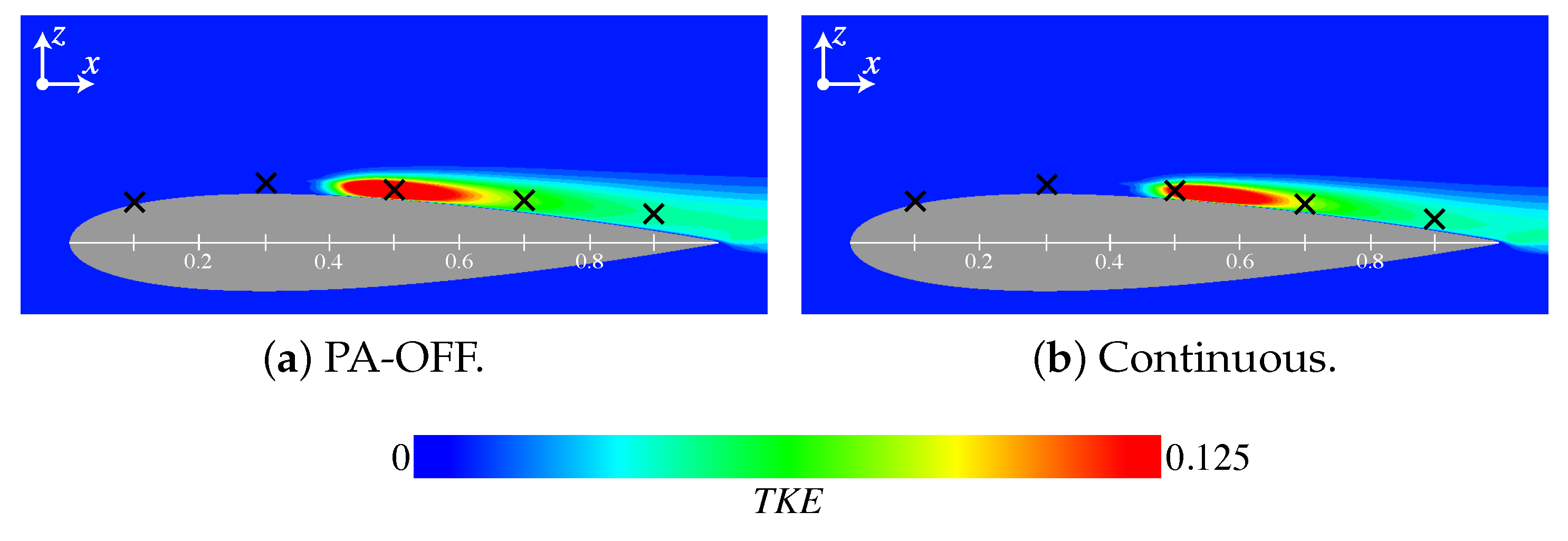
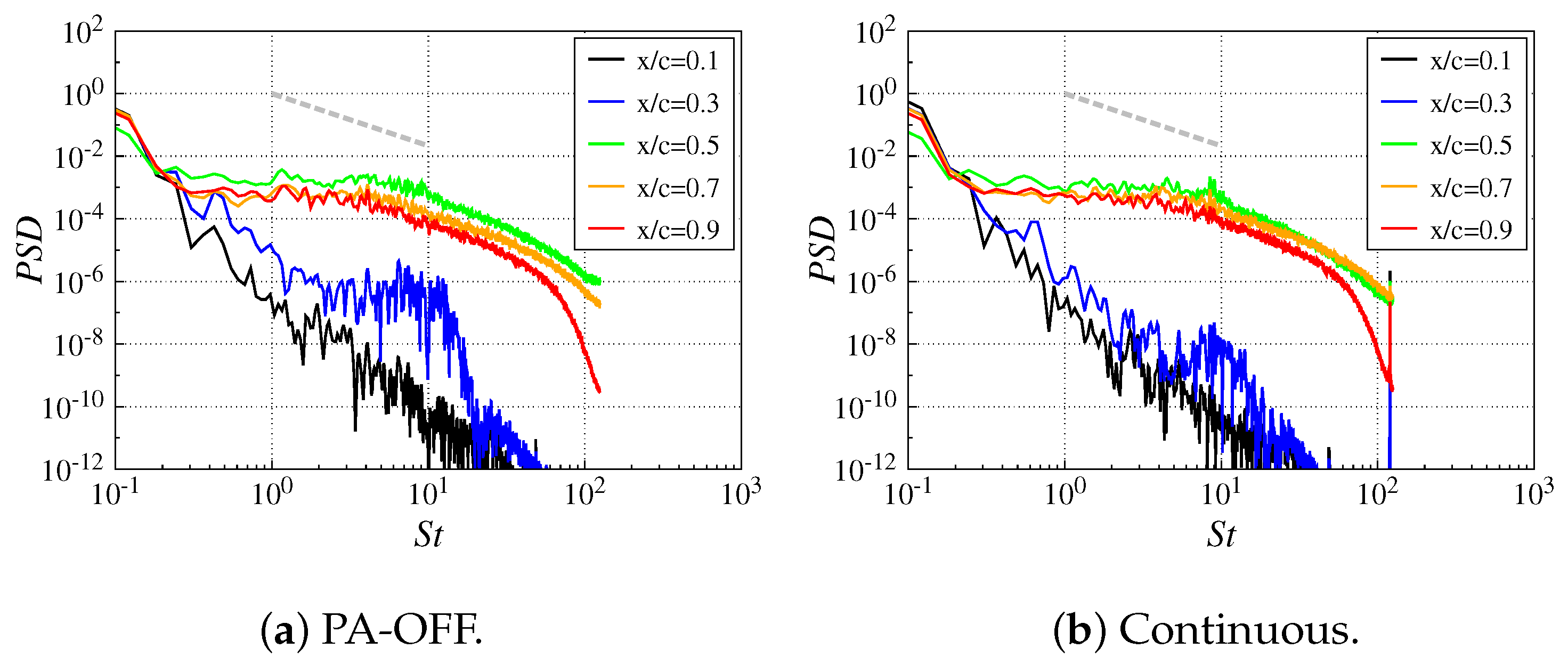
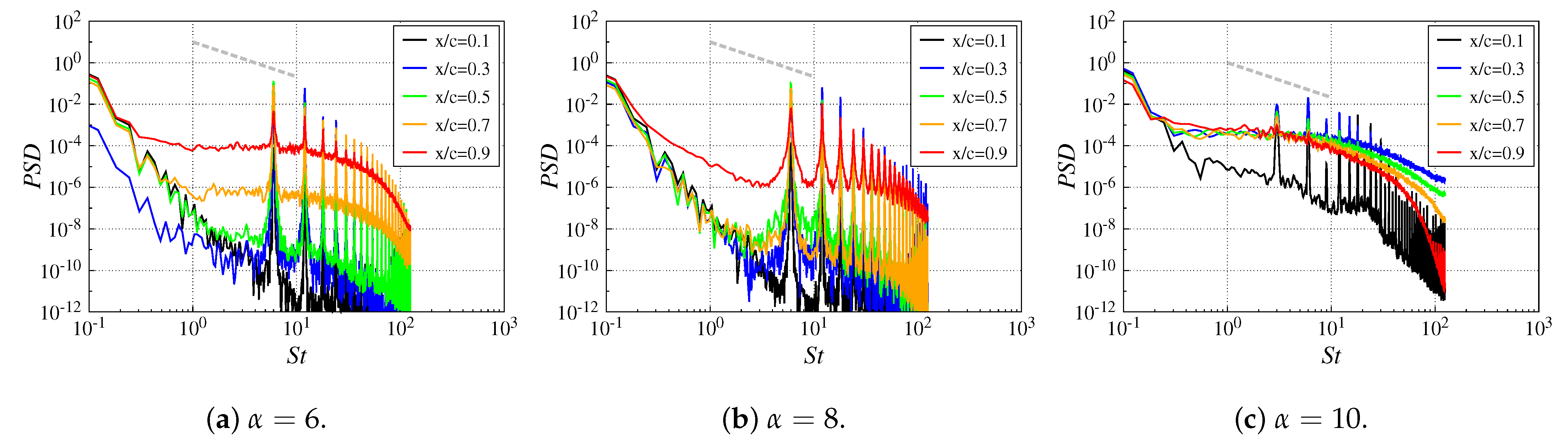
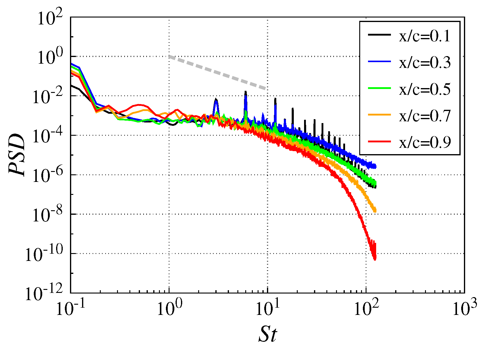
4.4. Unsteady Flow Feature

In this section, we discuss the relationship between the instantaneous flow field for each case and the plots up to Section 4.3. Figure 13 shows the instantaneous flow fields of the PA-OFF and Continuous cases at $\alpha =6$. The isosurface is the second invariant of the velocity gradient tensor ($Q=6250$), colored by the chordwise velocity (u/$U_{\infty }$). Figure 14 and Figure 15 show the turbulent-kinetic-energy (TKE) distributions and the power spectral densities (PSDs) of the chordwise velocity fluctuations of the PA-OFF and Continuous cases, respectively. The PSD shows the value at the position where the TKE is the largest (indicated by the black cross symbol in Figure 14) at each cord length position. The gray dashed line indicates the slope of Kolmogorov’s −5/3 power law. As shown in Figure 13, the instantaneous flow fields of the PA-OFF and Continuous cases are similar. In Figure 15, the spectrum shows a −5/3 power slope at $x/c=0.5$ and downstream there in both PA-OFF and Continuous cases, indicating the flow transitions to turbulent flow. Although, at first glance, the instantaneous fields of the PA-OFF and Continuous cases are very similar, due to the momentum addition by PA, the laminar flow separation in the Continuous case is delayed more than that in the PA-OFF case, as shown in Figure 10, and the separated shear layer of the Continuous case is closer to the airfoil surface. As a result, as shown in Figure 12a, the displacement thickness of the Continuous case is thinner than that of PA-OFF in most regions. The position of the turbulent transition in the Continuous case is delayed, and a region where TKE is high is seen downstream compared to that in the PA-OFF case. Although only the case at $\alpha =6$ was discussed here, the flow characteristics of the PA-OFF and Continuous cases are the same for other angles of attack.

Figure 16 shows the instantaneous flow fields of the burst case at each angle of attack. The isosurface is the second invariant of the velocity gradient tensor ($Q=6250$), colored by the chordwise velocity (u/$U_{\infty }$). The flow fields in the Burst cases differ from those in the PA-OFF and Continuous cases, where the large separated region is formed under the separated shear layer. At $\alpha =6$ and 8 in Figure 16, two-dimensional vortex structures are induced by the burst drive of PA near the leading edge and move downstream. These two-dimensional vortex structures maintain their spanwise shape up to near the trailing edge. Such stable two-dimensional vortex structures are not observed in the controlled flows at post-stall angles. These two-dimensional vortex structures merge several times in the process of moving. Where large two-dimensional vortex structures merge, local variations of $C_{\mathrm{f}}$ and $C_{\mathrm{p}}$ are seen. Specifically, in the region of $0.4\lesssim x/c\lesssim 0.5$, a small plateau region is seen in Figure 9a,b, and a local decrease in $C_{\mathrm{f}}$ is seen in Figure 10a,b.

The difference between the flow fields at $\alpha =6$ and $\alpha =8$ is remarkable near the trailing edge. As shown in Figure 16b, the flow at $\alpha =8$ separates near the trailing edge while maintaining the two-dimensional vortex structures. The flow at $\alpha =10$ is different from those at $\alpha =6$ and 8, the two-dimensional vortex structures induced by PA rapidly collapse into the two-dimensional vortex structures (Figure 16c). This flow resembles the controlled flows investigated in the previous study [8] at the post-stall angles.

Figure 17 and Figure 18 show the TKE distributions and the PSDs of the chordwise velocity fluctuations for the Burst case at each angle of attack. The PSD shows the value at the position where the TKE is the largest (indicated by the black cross symbol in Figure 17) at each cord length position. The TKE distribution differs at each angle of attack, reflecting the characteristics of the instantaneous flow fields. At $\alpha =6$, the TKE increases from $x/c\simeq 0.3$ toward downstream due to the passing of the two-dimensional vortex structures. A turbulent transition occurs at $0.7\lesssim x/c\lesssim 0.8$, and the region where TKE is particularly high (red region) locally spreads. In the PSD of Figure 18a, at $x/c=0.3$, the frequency $St=6$ and its harmonics are dominant due to the passing of the two-dimensional vortex structures induced by the burst drive of PA. At $x/c=0.7$, the energy in the high-frequency range begins to increase due to the turbulent transition, and at $x/c=0.9$, a PSD decay of the −5/3 slope can be confirmed. The position, where the −5/3 slope reveals, is downstream of that in the PA-OFF case (Figure 15a). These PSD characteristics indicate that transporting the two-dimensional vortex structures suppresses the turbulent transition. At $\alpha =8$, the TKE increases from $x/c\simeq 0.2$ by the passing of the two-dimensional vortex structures, similar to that at $\alpha =6$. At $x/c\simeq 0.8$, the two-dimensional vortex structures begin to move away from the airfoil surface; thus, the high TKE region is also seen away from the airfoil surface. The two-dimensional vortex structures are relatively stable compared to those at the other angles of attack, and the turbulent transition is suppressed. Therefore, even at $x/c=0.9$, the PSD decay of the −5/3 slope is not seen (Figure 18b). At $\alpha =10$, TKE increases sharply at $0.1\lesssim x/c\lesssim 0.3$ due to rapid turbulent transition. The PSD also has high energy in the high-frequency range at $x/c=0.3$, and the slope of the energy decay is close to the −5/3 slope.

In Section 4.3, the possibility that the trailing edge separation affects the peak value of $C_{\mathrm{p}}$ at $\alpha =8$ in the burst case is discussed. At $\alpha =8$, as shown in Figure 16b and Figure 18b, the two-dimensional vortex structures induced by PA keep their structure and move away from the airfoil surface, near the trailing edge, while the flows in the burst cases at $\alpha =6$ and 8 occur as turbulent transitions and maintain attached near the trailing edge. Therefore, the promotion of turbulent transition at $\alpha =8$ could suppress the trailing edge separation, the negative $C_{\mathrm{p}}$ peak value could become lower, and $C_{\mathrm{L}}$ could be improved.

In the previous study [27], the control effects of $F^{+}=1$ and 10 were discussed by performing LESs at the angle of attack of $\alpha =6$. In the case of $F^{+}=1$, a turbulent transition occurred relatively upstream after a large-scale two-dimensional vortex structure shedding, while in the case of $F^{+}=10$, two-dimensional vortex structures keep their structures flowing up to the trailing edge of the airfoil. This result suggests the possibility of promoting a turbulence transition by using frequencies lower than the burst frequency, which induces stable two-dimensional structures, in a flow with a relatively small pressure gradient at low angles of attack. In other words, for the Bust case at $\alpha =8$ of the present study, using frequencies lower than $F^{+}=6$ could promote the turbulent transition and reduce the low-velocity region at the trailing edge. The characteristics of the controlled flow at the pre-stall condition differ depending on the angle of attack and the PA drive condition. A method of dynamically changing the PA drive method depending on the flow conditions at post-stall angles of attack to select an optimum PA drive is proposed [50]. If the optimum control method can be dynamically selected according to the flow conditions, even at pre-stall angles of attack, further improvements in aerodynamic characteristics could be expected.

4.5. Comparison with Controlled Flow at Post-Stall Angle of Attack

This section discusses the differences between the controlled flows at the pre- and post-stall angles of attack.

Figure 19 shows $C_{\mathrm{p}}$ and $C_{\mathrm{f}}$ distributions at the post-stall angle of attack ($\alpha =12$). In the PA-OFF case, a massive separation occurs from the leading edge of the airfoil, and thus, the $C_{\mathrm{p}}$ shows a flat distribution on the suction side, and the $C_{\mathrm{f}}$ value takes a negative value on most of the airfoil surface. Because of the massive separation, the $C_{\mathrm{L}}$ of the PA-OFF case is significantly lower compared to the pre-stall angles (Figure 7a). The burst drive with $F^{+}$ can suppress the massive flow separation and create flow reattachment, while the continuous drive cannot. The flow reattachment in the Burst case increases the $C_{\mathrm{L}}$ and decreases the $C_{\mathrm{D}}$ significantly. Both the $C_{\mathrm{L}}$ increase and $C_{\mathrm{D}}$ decrease contribute to $L/D$ improvement, as shown in Figure 6 and Figure 7. The detailed discussion may be found in [15]. On the other hand, at the pre-stall angles of attack, in the PA-OFF case, a separation bubble, which does not exist at the post-stall angle of attack, is formed on the airfoil’s upper surface, and its position and size affect the aerodynamic coefficients, as discussed in Section 4.3. The change in the separation bubble by PA control does not contribute much to the $C_{\mathrm{L}}$ increase but mainly reduces the $C_{\mathrm{D}}$ and contributes to the increase in $L/D$ (Figure 6 and Figure 7). At $\alpha =4$ and 8, the $C_{\mathrm{L}}$ decreases due to the shrink of the separation bubble, but the $C_{\mathrm{D}}$ reduction is larger than the $C_{\mathrm{L}}$ decrease, so the $L/D$ increases.

The difference in the flows in the Burst case at each angle of attack becomes more apparent when the discussion includes the instantaneous flow at $\alpha =12$. Figure 20 shows the instantaneous flow of the Burst case at $\alpha =12$. This flow resembles that at $\alpha =10$ shown in Figure 16c. The two-dimensional vortex structures induced by PA rapidly break down into fine vortices. Figure 21 and Figure 22 show the TKE distributions and the PSDs of the chordwise velocity fluctuations for the Burst case at $\alpha =12$. The PSD shows the value at the position where the TKE is the largest (indicated by the black cross symbol in Figure 21) at each cord length position. The region where TKE is locally high is seen at $0.1\lesssim x\lesssim 0.4$, and a PSD decay of the −5/3 slope is seen at all stations in Figure 22 because the turbulent transition rapidly occurs. The turbulence growth shown by these TKE and PSDs also resembles those at $\alpha =10$. The rapid turbulent transition draws the shear layer and reduces the separation region. On the other hand, as discussed in Section 4.4, at the lower angles of attack ($\alpha =$ 4, 6, and 8), the burst actuation induces the two-dimensional vortices, which maintain their spanwise shape (Figure 16). The transport of the two-dimensional vortices draws the shear layer to the airfoil surface and shrinks the separation bubble. Additionally, those two-dimensional vortices suppress the turbulent transition. The suppression of turbulence transition can be confirmed by the spectrum in Figure 18.

As discussed above, the control mechanism is different between near the stall angle of attack ($\alpha =10$ and 12) and at lower angles of attack ($\alpha =$ 4, 6, and 8). This may be because the pressure gradient on the airfoil surface increases as the angle of attack increases. The pressure gradient may promote the collapse of the two-dimensional vortices induced by PA near the stall angle of attack. For post-stall angle flows, previous studies [15,21] have shown that using $F^{+}\simeq 1$ maintains large two-dimensional vortex structures up to downstream. On the other hand, in the case of $F^{+}=6$, the two-dimensional vortex structures are maintained up to downstream at the low angles of attack in the present study. Whether or not the two-dimensional vortex structure is maintained may be determined by the relationship with the pressure gradient on the airfoil surface, and further research on this relationship is required.

Note that the magnitude of the pressure gradient on an airfoil surface depends on not only the angle of attack but also the curvature of the airfoil surface. For relatively thin airfoils, the flow control mechanism may differ from the cases of the NACA0015 airfoil. Further research on the relationship between the airfoil geometry and the flow control mechanism is required.

5. Conclusions

LES of the flows controlled by PA over an NACA0015 airfoil was performed at angles of attack before a stall. The flow control authority of PA was investigated, and the relationship between the aerodynamic coefficient and the flow field was clarified through the LES results.

The Continuous and Burst cases using PA at the angles of attack before the stall improved $L/D$ compared to PA-OFF. The improvement in $L/D$ is mainly owing to the reduction in $C_{{\mathrm{D}}_{\mathrm{p}}}$ in addition to the improvement in $C_{\mathrm{L}}$. The primary causes of the reduction in $C_{{\mathrm{D}}_{\mathrm{p}}}$ are (1) lower pressure at the suction peak and (2) reduction in the plateau region of $C_{\mathrm{p}}$ as the separation bubble is moved or shrunk on the upper surface of the airfoil. The second effect is remarkable in the Burst cases with $F^{+}=6$. Although, in the Bust case, the lift-to-drag ratio is improved at all angles of attack, the phenomena leading to the improvement differ between near-stall angles ($\alpha =10$ and 12) and other lower angles ($\alpha =4,6$, and 8). At near-stall angles, the turbulent transition is rapidly promoted by PA, and the flow is reattached. Whereas, at lower angles, the transport of two-dimensional vortex structures, which maintain their structures downstream and suppress the turbulent transition, creates flow reattachment. At $\alpha =4$ and 8, the $L/D$ of the Continuous case was higher than that of the Burst case because the suction peak value of $C_{\mathrm{p}}$ in the Burst case was not improved compared to the PA-OFF case due to the trailing edge separation. The trailing edge separation may be caused by the suppression of the turbulent transition by the two-dimensional vortices whose structures are maintained even near the trailing edge in addition to the reverse pressure gradient. Therefore, applying flow control methods that promote turbulence transition could possibly suppress the trailing separation and improve aerodynamic characteristics. Based on the results of the previous study [27], frequencies lower than $F^{+}=6$ may be effective, and further investigation is required. In addition, a control method that dynamically changes the PA drive conditions according to the angle of attack is needed for robust control.

It should be noted that these phenomena in the present study would depend on the airfoil geometry and flow conditions. Future studies on the influence of the airfoil geometry such as a thin airfoil and the flow conditions such as freestream turbulence are required.

References

1. Corke, T.C.; Enloe, C.L.; Wilkinson, P.S. Dielectric Barrier Discharge Plasma Actuators for Flow Control. Annu. Rev. Fluid Mech. 2010, 42, 505–529. [Google Scholar] [CrossRef]
2. Jukes, T.N.; Choi, K.S. Control of unsteady flow separation over a circular cylinder using dielectricbarrier-discharge surface plasma. Phys. Fluids 2009, 21, 094106. [Google Scholar] [CrossRef]
3. Greenblatt, D.; Schneider, T.; Schuele, C.Y. Mechanism of flow separation control using plasma actuation. Phys. Fluids 2012, 24, 077102. [Google Scholar] [CrossRef]
4. Post, M.L.; Corke, T.C. Separation Control on High Angle of Attack Airfoil Using Plasma Actuators. AIAA J. 2004, 42, 2177–2184. [Google Scholar] [CrossRef]
5. Jukes, T.N.; Choi, K.S.; Johnson, G.A.; Scott, S.J. Turbulent Drag Reduction by Surface Plasma through Spanwise Flow Oscillation. In Proceedings of the 3rd AIAA Flow Control Conference, San Francisco, CA, USA, 5–8 June 2006. AIAA-2006-3693. [Google Scholar] [CrossRef]
6. Visbal, M.R.; Gaitonde, D.V.; Roy, S. Control of Transitional and Turbulent Flows Using Plasma-Based Actuators. In Proceedings of the 36th AIAA Fluid Dynamics Conference and Exhibit, San Francisco, CA, USA, 5–8 June 2006. AIAA-2006-3230. [Google Scholar] [CrossRef]
7. Bénard, N.; Jolibois, J.; Moreau, E. Lift and drag performances of an axisymmetric airfoil controlled by plasma actuator. J. Electrost. 2009, 67, 133–139. [Google Scholar] [CrossRef]
8. Sato, M.; Nonomura, T.; Okada, K.; Asada, K.; Aono, H.; Yakeno, A.; Abe, Y.; Fujii, K. Mechanisms for laminar separated-flow control using dielectric-barrier-discharge plasma actuator at low Reynolds number. Phys. Fluids 2015, 27, 1–29. [Google Scholar] [CrossRef]
9. Thomas, F.O.; Corke, T.C.; Duong, A.; Midya, S.; Yates, K. Turbulent drag reduction using pulsed-DC plasma actuation. J. Phys. D Appl. Phys. 2019, 52, 434001. [Google Scholar] [CrossRef]
10. Wang, J.J.; Choi, K.S.; Feng, L.H.; Jukes, T.N.; Whalley, R.D. Recent developments in DBD plasma flow control. Prog. Aerosp. Sci. 2013, 62, 52–78. [Google Scholar] [CrossRef]
11. Vernet, J.A.; Orlu, R.; Soderblom, D.; Elofsson, P. Plasma Streamwise Vortex Generators for Flow Separation Control on Trucks. Flow Turbul. Combust. 2018, 100, 1101–1109. [Google Scholar] [CrossRef]
12. Zhang, Z.; Wu, Y.; Jia, M.; Song, H.; Sun, Z.; Zong, H.; Li, Y. The multichannel discharge plasma synthetic jet actuator. Sens. Actuators A Phys. 2017, 253, 112–117. [Google Scholar] [CrossRef]
13. Bhattacharya, S.; Gregory, J.W. Effect of Three-Dimensional Plasma Actuation on the Wake of a Circular Cylinder. AIAA J. 2015, 53, 958–967. [Google Scholar] [CrossRef]
14. Feng, L.H.; Jukes, N.T.; Choi, K.S.; Wang, J.J. Flow control over a NACA 0012 airfoil using dielectric-barrier-discharge plasma actuator with a Gurney flap. Exp. Fluids 2012, 52, 1533–1546. [Google Scholar] [CrossRef]
15. Fujii, K. Three Flow Feature behind the Flow Control Authority of DBD Plasma Actuator: Result of High-Fidelity Simulations and the Related Experiments. Appl. Sci. 2018, 8, 546. [Google Scholar] [CrossRef]
16. Wang, L.; Wong, C.W.; Alam, M.M.; Zhou, Y. Post-stall flow control using a sawtooth plasma actuator in burst mode. Aerosp. Sci. Technol. 2020, 107, 106251. [Google Scholar] [CrossRef]
17. Riherd, M.; Roy, S. Serpentine geometry plasma actuators for flow control. J. Appl. Phys. 2013, 114, 083303. [Google Scholar] [CrossRef]
18. Segawa, T.; Matsunuma, T. Applications of String-type DBD Plasma Actuators for Flow Control in Turbomachineries. In Proceedings of the 52nd Aerospace Sciences Meeting, National Harbor, Md, USA, 13–17 January 2014. AIAA 2014-1126. [Google Scholar] [CrossRef]
19. Kolbakir, C.; Hu, H.; Liu, Y.; Hu, H. An experimental study on different plasma actuator layouts for aircraft icing mitigation. Aerosp. Sci. Technol. 2020, 107, 106325. [Google Scholar] [CrossRef]
20. Visbal, M.R. Strategies for control of transitional and turbulent flows using plasma-based actuators. Int. J. Comput. Fluid Dyn. 2010, 24, 237–258. [Google Scholar] [CrossRef]
21. Ebrahimi, A.; Hajipour, M. Flow separation control over an airfoil using dual excitation of DBD plasma actuators. Aerosp. Sci. Technol. 2018, 79, 658–668. [Google Scholar] [CrossRef]
22. Wu, B.; Gao, C.; Liu, F.; Xue, M.; Zheng, B. Simulation of NACA0015 flow separation controlby burst-mode plasma actuation. Phys. Plasmas 2019, 26, 063507. [Google Scholar] [CrossRef]
23. Sato, M.; Aono, H.; Yakeno, A.; Nonomura, T.; Fujii, K.; Okada, K.; Asada, K. Multifactorial Effects of Operating Conditions of Dielectric-Barrier-Discharge Plasma Actuator on Laminar-Separated-Flow Control. AIAA J. 2015, 53, 2544–2559. [Google Scholar] [CrossRef]
24. Liu, R.; Niu, Z.; Wang, M.; Hao, M.; Lin, Q. Aerodynamic control of NACA 0021 airfoil model with spark discharge plasma synthetic jets. Sci. China Technol. Sci. 2015, 58, 1949–1955. [Google Scholar] [CrossRef]
25. Erfani, R.; Kontis, K. MEE-DBD Plasma Actuator Effect on Aerodynamics of a NACA0015 Aerofoil: Separation and 3D Wake. Comput. Methods Appl. Sci. 2019, 28. [Google Scholar] [CrossRef]
26. Cui, Y.; Zhao, Z.; Zheng, J.; Li, J.M.; Khoo, B.C. Separation Control over a NACA0015 Airfoil Using Nanosecond Pulsed Plasma Actuator. In Proceedings of the 55th AIAA Aerospace Sciences Meeting, Grapevine, TX, USA, 9–13 January 2017. AIAA-2017-0715. [Google Scholar] [CrossRef]
27. Asano, K.; Sato, M.; Nonomura, T.; Oyama, A.; Fujii, K. Control of Airfoil Flow at Cruise Condition by DBD Plasma Actuator- Sophisticated Airfoil vs. In Simple Airfoil with Flow Control. In Proceedings of the 8th AIAA Flow Control Conference, Washington, DC, USA, 13–17 June 2016. AIAA-2016-3624. [Google Scholar] [CrossRef]
28. Ogawa, T.; Asada, K.; Tatsukawa, T.; Fujii, K. Computational Analysis of the Control Authority of Plasma Actuators for Airfoil Flows at Low Angle of Attack. In Proceedings of the AIAA Scitech 2020 Forum, Orlando, FL, USA, 6–10 January 2020. AIAA 2020-0578. [Google Scholar] [CrossRef]
29. Asada, K.; Ninomiya, Y.; Oyama, A.; Fujii, K. Airfoil Flow Experiment on the Duty Cycle of DBD Plasma Actuator. In Proceedings of the 47th AIAA Aerospace Sciences Meeting including The New Horizons Forum and Aerospace Exposition, Orlando, FL, USA, 5–8 January 2009. AIAA-2009-531. [Google Scholar] [CrossRef]
30. Sekimoto, S.; Nonomura, T.; Fujii, K. Burst-Mode Frequency Effects of Dielectric Barrier Discharge Plasma Actuator for Separation Control. AIAA J. 2017, 55, 1385–1392. [Google Scholar] [CrossRef]
31. Sekimoto, S.; Fujii, K.; Hosokawa, S.; Akamatsu, H. Flow-control capability of electronic-substrate-sized power supply for a plasma actuator. Sens. Actuators A Phys. 2020, 306, 111951. [Google Scholar] [CrossRef]
32. Aono, H.; Sekimoto, S.; Sato, M.; Yakeno, A.; Nonomura, T.; Fujii, K. Computational and experimental analysis of flow structures induced by a plasma actuator with burst modulations in quiescent air. Mech. Eng. J. 2015, 2, 1–16. [Google Scholar] [CrossRef]
33. Sato, M.; Okada, K.; Aono, H.; Asada, K.; Yakeno, A.; nd Kozo Fujii, T.N. LES of Separated-flow Controlled by DBD Plasma Actuator around NACA 0015 over Reynolds Range of 104–106. In Proceedings of the 53rd AIAA Aerospace Sciences Meeting, Kissimmee, FL, USA, 5–9 January 2015. AIAA 2015-0308. [Google Scholar] [CrossRef]
34. Suzen, Y.B.; Huang, P.G. Simulations of Flow Separation Contorl using Plasma Actuator. In Proceedings of the 44th AIAA Aerospace Sciences Meeting and Exhibit, Reno, NV, USA, 9–12 January 2006. AIAA-2006-877. [Google Scholar] [CrossRef]
35. Font, G.I.; Enloe, C.L.; McLaughlin, T.E. Plasma Volumetric Effects on the Force Production of a Plasma Actuator. AIAA J. 2010, 48, 1869–1874. [Google Scholar] [CrossRef]
36. Chen, D.; Asada, K.; Sekimoto, S.; Fujii, K.; Nishida, H. A high-fidelity body-force modeling approachfor plasma-based flow control simulations. Phys. Fluids 2021, 33, 037115. [Google Scholar] [CrossRef]
37. Pereira, R.; Ragni, D.; Kotsonis, M. Effect of external flow velocity on momentum transfer of dielectric barrier discharge plasma actuators. J. Appl. Phys. 2014, 103301. [Google Scholar] [CrossRef]
38. Kawai, S.; Fujii, K. Analysis and Prediction of Thin-Airfoil Stall Phenomena Using Hybrid Turbulent Methodology. AIAA J. 2005, 43, 953–961. [Google Scholar] [CrossRef]
39. Kojima, R.; Nonomura, T.; Oyama, A.; Fujii, K. Large-Eddy Simulation of Low-Reynolds-Number Flow Over Thick and Thin NACA Airfoils. J. Aircr. 2013, 50, 187–196. [Google Scholar] [CrossRef]
40. Lee, D.; Kawai, S.; Nonomura, T.; Anyoji, M.; Aono, H.; Oyama, A.; Asai, K.; Fujii, K. Mechanisms of surface pressure distribution within a laminar separation bubble at different Reynolds numbers. Phys. Fluids 2015, 27, 023602. [Google Scholar] [CrossRef]
41. Lele, S.K. Compact Finite Difference Schemes with Spectral-like Resolution. J. Comput. Phys. 1992, 103, 16–42. [Google Scholar] [CrossRef]
42. Gaitonde, D.V.; Visbal, M.R. Padé-Type Higher-Order Boundary Filters for the Navier-Stokes Equations. AIAA J. 2000, 38, 2103–2112. [Google Scholar] [CrossRef]
43. Visbal, M.R.; Rizzetta, D.P. Large-Eddy Simulation on Curvilinear Grids Using Compact Differencing and Filtering Schemes. J. Fluids Eng. 2002, 124, 836–847. [Google Scholar] [CrossRef]
44. Fujii, K. Simple Ideas for the Accuracy and Efficiency Improvement of the Compressible Flow Simulation Methods. In Proceedings of the International CFD Workshop on Supersonic Transport Design, Tokyo, Japan, 16 March 1998; pp. 20–28, (later published as JAXA-SP-06-029E, pp. 25–28). [Google Scholar]
45. Choi, H.; Moin, P. Effects of the Computational Time Step on Numerical Solutions of Turbulent Flow. J. Comput. Phys. 1994, 113, 1–4. [Google Scholar] [CrossRef]
46. Visbal, M.R.; Rizzetta, D.P. Large-eddy Simulation on General Geometries Using Compact Differencing and Filtering Schemes. In Proceedings of the 40th AIAA Aerospace Sciences Meeting & Exhibit, Reno, NV, USA, 14–17 January 2002. AIAA-2002-288. [Google Scholar] [CrossRef]
47. Rizzetta, D.P.; Visbal, M.R.; Gaitonde, D.V. Large-Eddy Simulation of Supersonic Compression-Ramp Flow by High-Order Method. AIAA J. 2001, 39, 2283–2292. [Google Scholar] [CrossRef]
48. Kawai, S.; Fujii, K. Compact Scheme with Filtering for Large-Eddy Simulation of Transitional Boundary Layer. AIAA J. 2008, 46, 690–700. [Google Scholar] [CrossRef]
49. Fujii, K. Unified Zonal Method Based on the Fortified Solution Algorithm. J. Comput. Phys. 1995, 118, 92–108. [Google Scholar] [CrossRef]
50. Ogawa, T.; Asada, K.; Sekimoto, S.; Tatsukawa, T.; Fujii, K. Dynamic Burst Actuation to Enhance the Flow Control Authority of Plasma Actuators. MDPI Aerospace 2021, 8, 396. [Google Scholar] [CrossRef]
Figure 1. Schematic diagram of the DBD plasma actuator (PA) and the example of practical applications.
Applsci 12 09073 g001
Figure 2. Alternating current (AC) voltage waveform for the burst actuation.
Applsci 12 09073 g002
Figure 3. Distribution of body force in the x direction based on the Suzen–Huang model [34] and body force vectors near PA. Gray and orange areas represent the airfoil surface and exposed electrode, respectively.
Applsci 12 09073 g003
Figure 4. Computational grids and domain. The grids were visualized for every four points.
Applsci 12 09073 g004
Figure 5. Pressure coefficient ( C p ) distributions around the airfoil in each case of the computations (CFDs) and experiments (EXPs).
Applsci 12 09073 g005
Figure 6. Lift-to-drag ratio ( L / D ) versus angle of attack ( α ).
Applsci 12 09073 g006
Figure 7. Lift coefficient ( C L ) and drag coefficient ( C D ) versus angle of attack ( α ).
Applsci 12 09073 g007
Figure 8. Pressure drag coefficient ( C D p ) versus angle of attack ( α ).
Applsci 12 09073 g008
Figure 9. Pressure coefficient ( C p ) distributions around the airfoil.
Applsci 12 09073 g009
Figure 10. Skin friction coefficient ( C f ) distributions on the airfoil’s upper surface.
Applsci 12 09073 g010
Figure 11. Time- and spanwise-averaged flows colored with the chordwise velocity (u/ U ).
Applsci 12 09073 g011
Figure 12. Displacement thickness ( δ * ) on the airfoil’s upper surface.
Applsci 12 09073 g012
Figure 13. Instantaneous flows with the isosurface of the second invariant of the velocity gradient tensor colored with the chordwise velocity (u/ U ) at α = 6 .
Applsci 12 09073 g013
Figure 14. Turbulent kinetic energy (TKE) distributions at α = 6 .
Applsci 12 09073 g014
Figure 15. Power spectrum densities (PSDs) of the chordwise velocity fluctuations at the point of the maximum TKE directly above each code length at α = 6 .
Applsci 12 09073 g015
Figure 16. Instantaneous flows with the isosurface of the second invariant of the velocity gradient tensor colored with the chordwise velocity (u/ U ) in the Burst cases.
Applsci 12 09073 g016
Figure 17. Turbulent kinetic energy (TKE) distributions in the Burst cases.
Applsci 12 09073 g017
Figure 18. Power spectrum densities (PSDs) of the chordwise velocity fluctuation at the point of the maximum TKE directly above each code length in the Burst cases.
Applsci 12 09073 g018
Figure 19. Pressure coefficient ( C p ) and skin friction coefficient ( C f ) distributions on the airfoil’s upper surface at α = 12 .
Applsci 12 09073 g019
Figure 20. Instantaneous flows with the isosurface of the second invariant of the velocity gradient tensor colored with the chordwise velocity (u/ U ) in the Burst cases at α = 12 .
Applsci 12 09073 g020
Figure 21. Turbulent kinetic energy (TKE) distribution in the Burst case at α = 12 .
Applsci 12 09073 g021
Figure 22. Power spectrum densities (PSDs) of the chordwise velocity fluctuation at the point of the maximum TKE directly above each code length in the Burst case at α = 12 .
Applsci 12 09073 g022