Existence and Stability of nT-Periodic Orbits in the Boost Converter

Abstract

In high load conditions, the boost converter presents some phenomena, such as chattering, chaos, subharmonics, and $nT$-periodic orbits, which require studying them with the aim of reducing the effects and improving the performance of these electronic devices. In this paper, sufficient conditions for the existence of $nT$-periodic orbits are analytically obtained and the system stability is evaluated using eigenvalues of the Jacobian matrix of the Poincaré application. It is demonstrated numerically that $1T$-periodic orbits occur for a broad range of $\gamma$ parameters. The research obtains a particular class of $2T$-periodic orbits in the boost converter and a formula that provides sufficient conditions for the existence of $nT$-periodic orbits with and without saturation in the duty cycle. In addition, an analysis of $nT$-periodic orbits is performed with a biparametric diagram. The system stability is computed using a variational equation that allows perturbation of the $1T$-periodic orbits. Moreover, an analytical calculation of the Floquet exponents is performed to determine the stability limit of the $1T$-periodic orbit. Finally, the phenomena found in this research are described according to the behavior of real applications encountered in previous literature.

1. Introduction

A wide variety of applications are used today that require conversion of direct current (DC) voltages. Therefore, DC converters take on great importance and allow power transfer at voltages that allow different applications. A DC converter is equivalent to a transformer that allows voltage variations at the output and can regulate them. There are varieties of drivers for stepping up (boost converter) or down (buck converter) the voltage. Both converters are efficient technologies that play an important role in transforming electrical applications [1].

Boost DC-DC converters are widely used for renewable energies [2], computer power sources, battery chargers, automotive lighting systems, and power factor correction [3]. This power converter presents high efficiency, low cost, ease of implementation, and versatility. However, boost DC-DC converters are highly nonlinear systems because they have a commutation device. In addition, the converter may slip into the discontinuous conduction mode in cases of low loads, which occur when the inductor current crosses zero. Moreover, bifurcation and chaotic events have been demonstrated in DC-DC converters because of the nonlinear switching actions and types of controllers [4,5,6,7].

The implementation of various control techniques helps test modern controllers, such as nonlinear control techniques [8]. Recently, techniques such as Zero Average Dynamics (ZAD) have been used to control DC-DC converters, as presented in [8,9,10], both for the pulse to the center and the pulse to the side. ZAD has been used to regulate different types of systems; for example, the authors in [8] described the design, robustness analysis, and implementation of a ZAD and sliding mode control (ZAD–SMC) for a multiphase step-down converter.

The ZAD–SMC operates at a fixed switching frequency and allows the implementation of an interleaving technique that provides current-ripple cancellation at the converter output. In addition, the control with ZAD has also been used to implement a buck converter in a field programmable gate array (FPGA) [10]; applying ZAD with a pulse on the side fulfills the requirement of the fixed switching frequency. Additionally, bifurcation analyses were performed to study the transition from periodicity to chaos [11] in buck and boost DC-DC converters operated with the ZAD control technique. Other results show robustness with low output error and a fixed switching frequency [12,13].

Additionally, the converter displays different behaviors when the parameters vary and their operating conditions are modified [14]. In previous research, some authors have analyzed the bifurcations to find the optimal range of parameter design in power converters, thus establishing the conditions under which the system exhibits changes in stability or periodicity (periodic, quasi-periodic, or chaotic orbits) [13,15,16]. Furthermore, the existence of saturated periodic orbits in the boost converter leads to the presence of the period addition phenomenon, which has been partially studied in [17] and reported in one-dimensional discrete dynamical systems. For example, an effective and efficient solution using an interleaved boost converter was proposed in [2], which was not limited to only mitigate or alleviate partial shading effects but can also to extract the maximum power available from the whole partially shaded photovoltaic system with 100 % mismatch loss index (MML).

Although the literature review shows that authors have dealt with the stability issues in power converters, they have not presented a detailed analysis of the existence of $nT$-periodic orbits and determined equations that define the problem. Therefore, this paper illustrates the conditions for the existence of $nT$-periodic orbits. The stability of the orbits is studied based on eigenvalues of the Jacobian matrix of the Poincaré application. Contributions in this paper are defined as follows:

• An exact formula is presented to provide sufficient conditions for the existence of $nT$-periodic orbits with and without saturation in the duty cycle.
• The application of Poincaré is generalized and an equation is presented that allows calculating the Jacobian matrix to determine the stability of the $nT$-periodic orbits. A wide range of the $\gamma$ parameter, $1T$- and $2T$-periodic orbits in the boost converter, and Floquet exponents are determined to analyze the stability limit of the $1T$-periodic orbit.
• A biparametric diagram that generates nT-periodic orbits is created to perform the analysis from $1T$- to $7T$-periodic orbits.
• The variational equation that admits the perturbation of the $1T$-periodic orbits is calculated to determine the system stability.

The paper is divided into three more sections. Section 3 presents the materials and methods, where the description of the boost converter and the mathematical model used in this research are presented. In addition, this section defines the duty cycle formulation and the discretization of the system. Moreover, the Poincaré map application is included to analyze the periodic orbits. Finally, the stability analysis is explained in this section to find the $nT$-periodic orbits. Section 4 illustrates the results of these methods applied to find the different periodic orbits and analyze the findings. Finally, the conclusions are included in the last section of the paper.

2. Materials and Methods

In this section, the materials and methods are focused on presenting the different mathematical models of the boost converter and the analytical techniques to create periodic orbits.

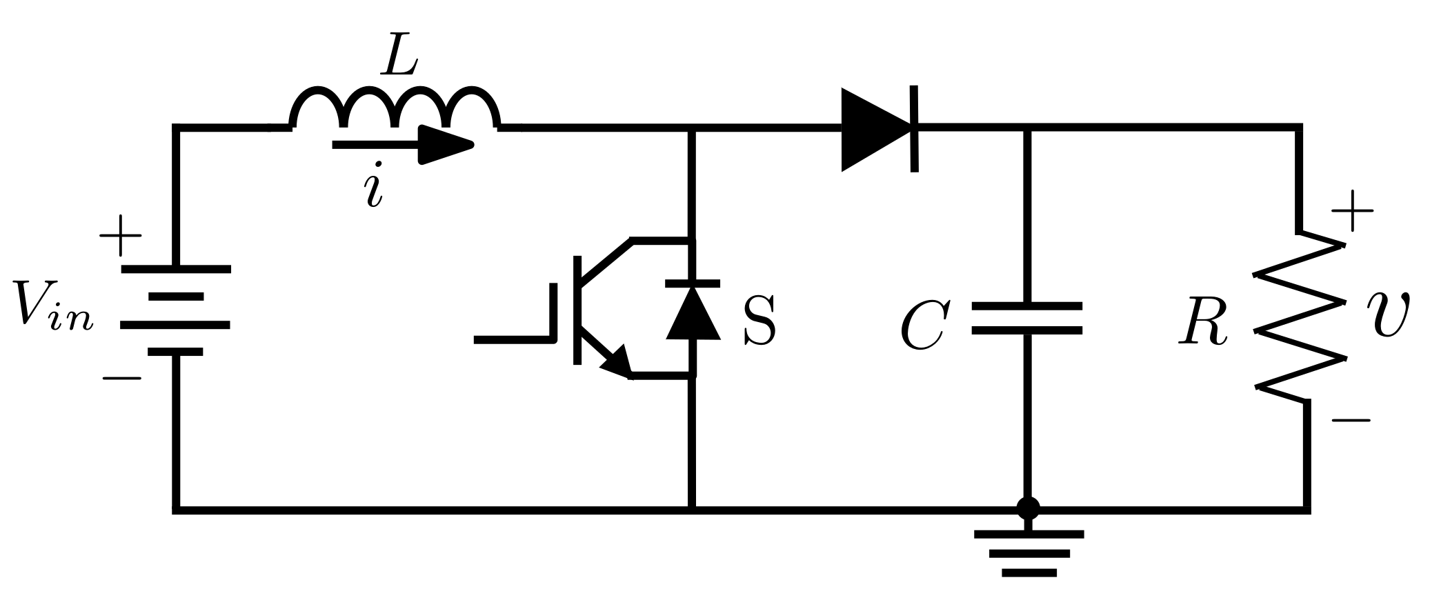
2.1. Boost Converter

The basic diagram of the boost converter is presented in Figure 1. The term $V_{in}$ is the input voltage, i is the current in the inductor L, S is the switch, D the diode, C the capacitance of the capacitor, and v the voltage at the load or output voltage. When the switch S is closed (ON), the coil L stores energy from the voltage source $V_{in}$, while the load is supplied through the capacitor C. When the switch is open (OFF), the current passes through the diode D and feeds the capacitor C and the load resistance R.

According to the diagram in Figure 1, the boost converter is governed by the differential expressions defined in Equations (1) and (2), where u is the control signal. The state space in which the system described by the boost converter evolves is a subset ${\mathbb{S}}^1\times {\mathbb{R}}^2$ (where ${\mathbb{S}}^1$ is the unit circle).

$$\begin{array}{cc}\hfill \frac{dv}{dt}& =-\frac{1}{RC}v+\frac{1}{C}i(1-u),\hfill \end{array}$$

(1)

$$\begin{array}{cc}\hfill \frac{di}{dt}& =-\frac{1}{L}v(1-u)+\frac{V_{in}}{L}.\hfill \end{array}$$

(2)

Equations (3)–(5) consider that $x_1$, $x_2$, and s are functions of the boost converter parameters, $V_{in}$, v, i, and the time t. In addition, those equations depend on the different parameters of the boost converter presented in Figure 1 and represented mathematically in Equations (1) and (2).

$$\begin{array}{c}\hfill x_1=\frac{v}{V_{in}},\end{array}$$

(3)

$$\begin{array}{c}\hfill x_2=\sqrt{\frac{L}{C}}\frac{i}{V_{in}},\end{array}$$

(4)

$$\begin{array}{c}\hfill s=\sqrt{LC}t.\end{array}$$

(5)

Next, a new expression is obtained by performing the first derivative of the variables defined in Equation (3) and represented in Equation (4) as ${\dot{x}}_1$ and ${\dot{x}}_2$. This equation can consider a parameter $\gamma =\sqrt{\frac{L}{R^{2}C}}$ to simplify the mathematical expression.

$$\left(\begin{array}{c}{\dot{x}}_1\\ {\dot{x}}_2\end{array}\right)=\left(\begin{array}{cc}-\gamma & 1-u\\ u-1& 0\end{array}\right)\left(\begin{array}{c}{x}_1\\ x_2\end{array}\right)+\left(\begin{array}{c}0\\ 1\end{array}\right).$$

(6)

From a theoretical perspective, as the boost converter is a voltage booster, $v>V_{in}$, so $x_1>1$. Therefore, when simulating the system, it is stated that the initial voltage condition must be strictly greater than 1. When u changes in the set $\{0,1\}$, a piecewise linear system is obtained, as represented in Equations (7) and (8).

$$\begin{array}{cc}\hfill \dot{X}\left(t\right)& =A_{1}X\left(t\right)+B,\mathrm{corresponding}\mathrm{to}u=1,\hfill \end{array}$$

(7)

$$\begin{array}{cc}\hfill \dot{X}\left(t\right)& =A_{2}X\left(t\right)+B,\mathrm{corresponding}\mathrm{to}u=0.\hfill \end{array}$$

(8)

This last expression is simplified by considering that the matrices $A_1$, $A_2$, and B have the terms presented in Equations (9)–(11). The terms consider the previously established parameter $\gamma$.

$$\begin{array}{c}\hfill A_1=\left(\begin{array}{cc}-\gamma & 0\\ 0& 0\end{array}\right),\end{array}$$

(9)

$$\begin{array}{c}\hfill A_2=\left(\begin{array}{cc}-\gamma & 1\\ -1& 0\end{array}\right),\end{array}$$

(10)

$$\begin{array}{c}\hfill B=\left(\begin{array}{c}0\\ 1\end{array}\right).\end{array}$$

(11)

Equations (7) and (8) represent the differential expressions given by the general Equation (12). This new expression is known as the control system, where $u\in \mathbb{R}$ is the variable control or system input [18].

$$\dot{X}=A_{1}X+B+(A_2-A_1)Xu.$$

(12)

The result of this expression is defined according to the topology of the system. Thus, the solution for each topology (u in the set $\{0,1\}$) can establish a solution in time by integrating the terms between $t_0$ and t (Equation (13)), where ${\varphi }_i(t-t_0)=e^{A_i(t-t_0)}$ and ${\psi }_i(t-t_0)={\displaystyle {\int }_{t_0}^t{e}^{A_i(t-\tau )}Bd\tau }$ [19].

$$X_i\left(t\right)={\varphi }_i(t-t_0)X\left(t_0\right)+{\psi }_i(t-t_0).$$

(13)

With each topology and the calculation of the exponential matrix, a new expression is established, as presented in Equation (14). Herein, the term $I_2$ is the identity matrix with a size of $2\times 2$.

$${\psi }_1(t-t_0)=B(t-t_0)\mathrm{and}{\psi }_2(t-t_0)=A_2^{-1}\left(e^{A_2(t-t_0)}-I_2\right)B.$$

(14)

In terms of each of the components, the solutions of the system in Equation (6) are:

• For the topology 1 ($u=1$):

  $$x_1\left(t\right)=x_1\left(t_0\right)e^{-\gamma (t-t_0)},$$

  (15)

  $$x_2\left(t\right)=x_2\left(t_0\right)+(t-t_0).$$

  (16)
• For the topology 2 ($u=0$):

  $$\begin{array}{c}\hfill x_1\left(t\right)=e^{-\frac{\gamma }{2}(t-t_0)}[\left(x_1\left(t_0\right)-1\right)cos\omega (t-t_0)\\ \hfill -\frac{\gamma }{2\omega }\left(x_1\left(t_0\right)-1-\frac{2}{\gamma }{x}_2\left(t_0\right)\right)sin\omega (t-t_0)]+1,\end{array}$$

  (17)

  $$\begin{array}{c}\hfill x_2\left(t\right)=e^{-\frac{\gamma }{2}(t-t_0)}[\left(x_2\left(t_0\right)-\gamma \right)cos\omega (t-t_0)\\ \hfill +\left(\frac{\gamma }{2\omega }\left(x_2\left(t_0\right)-\gamma \right)-\frac{1}{\omega }\left(x_1\left(t_0\right)-1\right)\right)sin\omega (t-t_0)]+\gamma .\end{array}$$

  (18)
  In these two expressions, the term $\omega =\frac{1}{2}\sqrt{4-{\gamma }^2}$. In addition, it is assumed that $4-{\gamma }^2>0$, which means that the relation $4R^{2}C>L$ must be fulfilled in the experimental test. In other words, this relationship must be fulfilled because if there is a very small load resistance R, the current in the load will tend towards infinity. The same thing happens if C is very small: the current in the capacitor will tend to infinity. Furthermore, if the inductance is too large, the current in the inductor will tend to infinity. All these behaviors are considered as unwanted solutions.
• Moreover, a topology 3 is obtained when inductor current ($i=0$), as expressed in the following equation:

  $$\begin{array}{cc}\hfill x_1\left(t\right)& =x_1\left(t_0\right)e^{-\gamma (t-t_0)},\hfill \\ \hfill x_2\left(t\right)& =0.\hfill \end{array}$$

  (19)
  However, this third topology corresponds to the discontinuous conduction mode. This research will not consider it, as the work focuses on performing analysis in the continuous condition mode.

2.2. Duty Cycle

The duty cycle is the percentage of time the system works and is created by a switching system. This formulation has been performed in previous research to determine the operation of the system [20]. The following expression for the duty cycle is obtained for the studied system and is denoted as $d_c$. This expression is calculated with the ZAD and symmetric centered PWM.

$$d_c={\displaystyle \frac{2s\left(\mathrm{x}\left(nT\right)\right)+T{\dot{s}}_2\left(\mathrm{x}\left(nT\right)\right)}{{\dot{s}}_2\left(\mathrm{x}\left(nT\right)\right)-{\dot{s}}_1\left(\mathrm{x}\left(nT\right)\right)}}.$$

(20)

where $d_c$ is the duty cycle calculated with the ZAD technique, T is the switching frequency of the switch S, n is a number that represents the periodic orbits, s is the value of the initial sliding surface in the time $nT$, ${\dot{s}}_2$ is the negative slope of the sliding surface, and ${\dot{s}}_1$ is the positive slope of the sliding surface [21]. The resulting value of calculating the duty cycle with the previous expression ($d_c$) can be $d_c<0$ or $d_c>T$. In both cases, the system saturates and a selection must be performed according to the following alternatives:

1.

If $d_c<0$, the system is forced to evolve according to the 1 topology.

2.

If $d_c>T$, the system is forced to evolve according to the 2 topology.

3.

The denominator of Equation (20) is equal to $k_1{x}_2\left(nT\right)-k_2{x}_1\left(nT\right)$, where $k_1$ and $k_2$ are control parameters with ZAD. If this expression is zero, the system is required to evolve according to the topology 1 if the numerator $2s\left(\mathrm{x}\left(nT\right)\right)+T{\dot{s}}_2\left(\mathrm{x}\left(nT\right)\right)>0$ and evolve according to the topology 2 if $2s\left(\mathrm{x}\left(nT\right)\right)+T{\dot{s}}_2\left(\mathrm{x}\left(nT\right)\right)<0$.

2.3. System Discretization

In a continuous dynamic system, discretization is accomplished by selecting an appropriate hyperplane at which the trajectories intersect at an angle other than zero (transversality condition) [22,23]. Thus, the Poincaré map is defined as in Equation (21). The term $P\left(x\right)$ is the intersection of the orbit passing through x with the hyperplane $\Sigma$.

$$\begin{array}{c}P:\Sigma \to \Sigma \hfill \\ x\mapsto P\left(x\right).\hfill \end{array}$$

(21)

Note that, if $L_0$ is a limit cycle, then the orbit through $x_0$ always intersects $\Sigma$ at $x_0$. Thus, a $1T$-periodic orbit corresponds to a single point in $\Sigma$; a $2T$-periodic orbit will correspond to 2 points in $\Sigma$; and so on. This is because our system is T-periodically forced. A sample of the system is taken each period to build the Poincaré application used to study the dynamics of the Boost converter, concatenating the solutions in each of the intervals $[nT,nT+\frac{d_n}{2}]$, $[nT+\frac{d_n}{2},(n+1)T-\frac{d_n}{2}]$, $[(n+1)T-\frac{d_n}{2},(n+1)T]$, where $d_n$ is the duty cycle at a point n, following the methodology presented in [16]. Equation (13) is used to achieve this, as follows:

If $\mathbf{x}\left(nT\right)$ is the state of the system at the time $nT$; then, at the end of the interval $[nT,nT+\frac{d_n}{2}]$:

$${\mathbf{x}}_1\left(nT+\frac{d_n}{2}\right)={\varphi }_1\left(\frac{d_n}{2}\right)\mathbf{x}\left(nT\right)+{\psi }_1\left(\frac{d_n}{2}\right).$$

(22)

Now, at the end of the second stretch $[nT+\frac{d_n}{2},(n+1)T-\frac{d_n}{2}]$:

$${\mathbf{x}}_2\left((n+1)T-\frac{d_n}{2}\right)={\varphi }_2\left(T-d_n\right){\mathbf{x}}_1\left(nT+\frac{d_n}{2}\right)+{\psi }_2\left(T-d_n\right).$$

(23)

Consequently, at the end of the second section:

$$\begin{array}{c}\hfill {\mathbf{x}}_2\left((n+1)T-\frac{d_n}{2}\right)={\varphi }_2\left(T-d_n\right){\varphi }_1\left(\frac{d_n}{2}\right)\mathbf{x}\left(nT\right)\\ \hfill +{\varphi }_2\left(T-d_n\right){\psi }_1\left(\frac{d_n}{2}\right)+{\psi }_2\left(T-d_n\right).\end{array}$$

(24)

Now, at the end of the third trace $[(n+1)T-\frac{d_n}{2},(n+1)T]$:

$${\mathbf{x}}_3\left((n+1)T\right)={\varphi }_1\left(\frac{d_n}{2}\right){\mathbf{x}}_2\left((n+1)T-\frac{d_n}{2}\right)+{\psi }_1\left(\frac{d_n}{2}\right).$$

(25)

Therefore, at the end of the third section:

$$\begin{array}{cc}\hfill {\mathbf{x}}_3\left((n+1)T\right)& ={\varphi }_1\left(\frac{d_n}{2}\right){\varphi }_2\left(T-d_n\right){\varphi }_1\left(\frac{d_n}{2}\right)\mathbf{x}\left(nT\right)\hfill \\ \hfill & +{\varphi }_1\left(\frac{d_n}{2}\right){\varphi }_2\left(T-d_n\right){\psi }_1\left(\frac{d_n}{2}\right)\hfill \\ \hfill & +{\varphi }_1\left(\frac{d_n}{2}\right){\psi }_2\left(T-d_n\right)+{\psi }_1\left(\frac{d_n}{2}\right).\hfill \end{array}$$

(26)

The Poincaré map P used in this research is that corresponding to

$$P\left(\mathbf{x}\left(nT\right)\right)={\mathbf{x}}_3\left((n+1)T\right).$$

The term ${\mathbf{x}}_3\left((n+1)T\right)$ is given by Equation (26). Note that in this case, no duty cycle saturation is assumed; however, $d_n\in \left(0,T\right)$ is assumed. When the duty cycle saturates, then:

1.

If $d_n=0$, the Poincaré map corresponds to

$$P\left(\mathbf{x}\left(nT\right)\right)={\varphi }_2\left(T\right)\mathbf{x}\left(nT\right)+{\psi }_2\left(T\right).$$

(27)

2.

If $d_n=T$, the Poincaré map corresponds to

$$P\left(\mathbf{x}\left(nT\right)\right)={\varphi }_1\left(T\right)\mathbf{x}\left(nT\right)+{\psi }_1\left(T\right).$$

(28)

Note that the Poincaré map P is a function of the state of the system at the instant $nT$ and of the duty cycle in the interval $\left[nT,(n+1)T\right]$, that is, $P=P\left(\mathbf{x}\left(nT\right),d_n\right)$. The latter must be considered when analyzing the stability of periodic orbits.

2.4. Stability of Periodic Orbits

The periodic orbits of the system displayed in Equation (6) correspond to the fixed points of the Poincaré map given by the relations shown in Equations (26)–(28). First, the fixed points of the Poincaré application are presented for the case where there is no saturation of the duty cycle.

Fixed points are those at which ${\mathbf{x}}_3\left((n+1)T\right)=\mathbf{x}\left(nT\right)$. This last equality can be used for Equation (26), determining sufficient conditions for the existence of $1T$ periodic orbits:

$$\begin{array}{cc}\hfill \mathbf{x}\left(nT\right)& ={\left[{\mathbf{I}}_2-{\varphi }_1\left(\frac{d_n}{2}\right){\varphi }_2\left(T-d_n\right){\varphi }_1\left(\frac{d_n}{2}\right)\right]}^{-1}·\hfill \\ \hfill & [{\varphi }_1\left(\frac{d_n}{2}\right){\varphi }_2\left(T-d_n\right){\psi }_1\left(\frac{d_n}{2}\right)\hfill \\ \hfill & +{\varphi }_1\left(\frac{d_n}{2}\right){\psi }_2\left(T-d_n\right)+{\psi }_1\left(\frac{d_n}{2}\right)].\hfill \end{array}$$

(29)

With this methodology, the existence of $1T$-periodic orbits is restricted to the invertibility of the matrix $\mathbf{A}={\mathbf{I}}_2-{\varphi }_1\left(\frac{d_n}{2}\right){\varphi }_2\left(T-d_n\right){\varphi }_1\left(\frac{d_n}{2}\right)$.

From a functional analysis, if the spectral radius of the matrix is less than 1, then the matrix $\mathbf{A}$ is invertible. Given an initial condition, this last matrix is a function of the duty cycle, and the latter is a function of $\gamma$.

$${\varphi }_1\left(\frac{d_n}{2}\right){\varphi }_2\left(T-d_n\right){\varphi }_1\left(\frac{d_n}{2}\right).$$

(30)

Fixing the period at $T=0.18s$ and varying $\gamma$ in the interval $\left(0.3,0.5\right)$, the spectral radius of the matrix ${\varphi }_1\left(\frac{d_n}{2}\right){\varphi }_2\left(T-d_n\right){\varphi }_1\left(\frac{d_n}{2}\right)$ is less than 1, and it follows that the matrix $\mathbf{A}$ is invertible. When the duty cycle is saturated, the following conditions for the existence of orbits are obtained:

$$\mathrm{if}{d}_n=0,\mathbf{x}\left(nT\right)={\left[{\mathbf{I}}_2-{\varphi }_2\left(T\right)\right]}^{-1}{\psi }_2\left(T\right),$$

(31)

$$\mathrm{if}{d}_n=T,\mathbf{x}\left(nT\right)={\left[{\mathbf{I}}_2-{\varphi }_1\left(T\right)\right]}^{-1}{\psi }_1\left(T\right).$$

(32)

As the spectral radius of the matrix ${\varphi }_1\left(T\right)$ is 1, Equation (12) is not applicable to determine orbits of period and in the case where the cycle saturates at T.

2.5. $2T$-Periodic Orbits

The $2T$-periodic orbits correspond to the 2-cycles of the Poincaré application. Three types of $2T$-periodic orbits are found: unsaturated, semi-saturated, and saturated. The mathematical expressions of these orbits are described as follows.

2.5.1. Unsaturated $2T$-Periodic Orbits

In this type of orbit, the duty cycles are not saturated. They belong to the interval $\left(0,T\right)$. We assume that the unsaturated 2-cycle corresponds to $\{{\mathbf{x}}_0,{\mathbf{x}}_1\}$. From Equation (26), the following expression is obtained:

$$\begin{array}{cc}\hfill {\mathbf{x}}_1\left((n+1)T\right)& ={\varphi }_1\left(\frac{d_n}{2}\right){\varphi }_2\left(T-d_n\right){\varphi }_1\left(\frac{d_n}{2}\right){\mathbf{x}}_0\left(nT\right)\hfill \\ \hfill & +{\varphi }_1\left(\frac{d_n}{2}\right){\varphi }_2\left(T-d_n\right){\psi }_1\left(\frac{d_n}{2}\right)\hfill \\ \hfill & +{\varphi }_1\left(\frac{d_n}{2}\right){\psi }_2\left(T-d_n\right)+{\psi }_1\left(\frac{d_n}{2}\right).\hfill \end{array}$$

(33)

Now,

$$\begin{array}{cc}\hfill {\mathbf{x}}_2\left((n+2)T\right)& ={\varphi }_1\left(\frac{{\tilde{d}}_n}{2}\right){\varphi }_2\left(T-{\tilde{d}}_n\right){\varphi }_1\left(\frac{{\tilde{d}}_n}{2}\right){\mathbf{x}}_1\left((n+1)T\right)\hfill \\ \hfill & +{\varphi }_1\left(\frac{{\tilde{d}}_n}{2}\right){\varphi }_2\left(T-{\tilde{d}}_n\right){\psi }_1\left(\frac{{\tilde{d}}_n}{2}\right)\hfill \\ \hfill & +{\varphi }_1\left(\frac{{\tilde{d}}_n}{2}\right){\psi }_2\left(T-{\tilde{d}}_n\right)+{\psi }_1\left(\frac{{\tilde{d}}_n}{2}\right).\hfill \end{array}$$

(34)

As no saturation is assumed in the duty cycles, then $d_n\in \left(0,T\right)$ and ${\tilde{d}}_n\in \left(0,T\right)$.

By considering ${\mathbf{x}}_0\left(nT\right)={\mathbf{x}}_2\left((n+2)T\right)$, the initial conditions for the existence of orbits and unsaturated $2T$-periodic orbits are obtained:

$${\mathbf{x}}_0\left(nT\right)={\left({\mathbf{I}}_2-\mathbf{A}\right)}^{-1}·\left(\mathbf{B}\left(\mathbf{C}+\mathbf{D}\right)+\mathbf{J}\right),$$

(35)

where:

$$\begin{array}{cc}\mathbf{A}\hfill & =\mathbf{B}·{\varphi }_1\left(\frac{d_n}{2}\right){\varphi }_2\left(T-d_n\right){\varphi }_1\left(\frac{d_n}{2}\right),\hfill \\ \mathbf{B}\hfill & ={\varphi }_1\left(\frac{{\tilde{d}}_n}{2}\right){\varphi }_2\left(T-{\tilde{d}}_n\right){\varphi }_1\left(\frac{{\tilde{d}}_n}{2}\right),\hfill \\ \mathbf{C}\hfill & ={\varphi }_1\left(\frac{d_n}{2}\right){\varphi }_2\left(T-d_n\right){\psi }_1\left(\frac{d_n}{2}\right),\hfill \\ \mathbf{D}\hfill & ={\varphi }_1\left(\frac{d_n}{2}\right){\psi }_2\left(T-d_n\right)+{\psi }_1\left(\frac{d_n}{2}\right),\hfill \\ \mathbf{J}\hfill & ={\varphi }_1\left(\frac{{\tilde{d}}_n}{2}\right){\varphi }_2\left(T-{\tilde{d}}_n\right){\psi }_1\left(\frac{{\tilde{d}}_n}{2}\right)+{\varphi }_1\left(\frac{{\tilde{d}}_n}{2}\right){\psi }_2\left(T-{\tilde{d}}_n\right)+{\psi }_1\left(\frac{{\tilde{d}}_n}{2}\right).\hfill \end{array}$$

(36)

Numerically, the matrix ${\mathbf{I}}_2-\mathbf{A}$ is invertible, as the spectral radius of the matrix $\mathbf{A}$ is less than 1. This shows that unsaturated $2T$-periodic orbits are found.

2.5.2. Semi-Saturated $2T$-Periodic Orbits

These correspond to the 2-cycles of the Poincaré map, in which one duty cycle belongs to the interval $\left(0,T\right)$ (it is not saturated) and the other saturates at T. Suppose that the $2-$ loop corresponds to $\{{\mathbf{x}}_0,{\mathbf{x}}_1\}$. Thus,

$$\begin{array}{cc}\hfill {\mathbf{x}}_1\left((n+1)T\right)& ={\varphi }_1\left(\frac{d_n}{2}\right){\varphi }_2\left(T-d_n\right){\varphi }_1\left(\frac{d_n}{2}\right){\mathbf{x}}_0\left(nT\right)\hfill \\ \hfill & +{\varphi }_1\left(\frac{d_n}{2}\right){\varphi }_2\left(T-d_n\right){\psi }_1\left(\frac{d_n}{2}\right)\hfill \\ \hfill & +{\varphi }_1\left(\frac{d_n}{2}\right){\psi }_2\left(T-d_n\right)+{\psi }_1\left(\frac{d_n}{2}\right).\hfill \end{array}$$

(37)

where $d_n\in \left(0,T\right)$.

By considering that ${\tilde{d}}_n=T$ and the relation in Equation (28), the expression in Equation (38) is obtained.

$$\begin{array}{c}\hfill {\mathbf{x}}_2\left((n+2)T\right)={\varphi }_1\left(T\right){\mathbf{x}}_1\left((n+1)T\right)+{\psi }_1\left(T\right).\end{array}$$

(38)

Again, by considering ${\mathbf{x}}_0\left(nT\right)={\mathbf{x}}_2\left((n+2)T\right)$, the initial conditions for the existence of semi-saturated $2T$-periodic orbits are defined in Equation (39).

$${\mathbf{x}}_0\left(nT\right)={\left({\mathbf{I}}_2-\mathbf{A}\right)}^{-1}·\left(\mathbf{B}+\mathbf{C}\right),$$

(39)

where

$$\mathbf{A}={\varphi }_1\left(T\right){\varphi }_1\left(\frac{d_n}{2}\right){\varphi }_2\left(T-d_n\right){\varphi }_1\left(\frac{d_n}{2}\right),$$

(40)

$$\mathbf{B}={\varphi }_1\left(T\right){\varphi }_1\left(\frac{d_n}{2}\right){\varphi }_2\left(T-d_n\right){\psi }_1\left(\frac{d_n}{2}\right),$$

(41)

$$\mathbf{C}={\varphi }_1\left(T\right)\left({\varphi }_1\left(\frac{d_n}{2}\right){\psi }_2\left(T-d_n\right)+{\psi }_1\left(\frac{d_n}{2}\right)\right)+{\psi }_1\left(T\right).$$

(42)

Numerically, the matrix $\left({\mathbf{I}}_2-\mathbf{A}\right)$ is invertible, as the spectral radius of the matrix $\mathbf{A}$ is smaller than 1.

2.5.3. Saturated $2T$-Periodic Orbits

This orbit corresponds to the 2-cycles of the Poincaré application. In this case, one duty cycle saturates at 0 and the other at T. Following the same procedure, suppose that the 2-cycle corresponds to $\{{\mathbf{x}}_0,{\mathbf{x}}_1\}$. From the relations defined in Equations (27) and (28), the expression of Equation (43) is obtained.

$${\mathbf{x}}_1\left((n+1)T\right)={\varphi }_2\left(T\right){\mathbf{x}}_0\left(nT\right)+{\psi }_2\left(T\right),$$

(43)

and

$${\mathbf{x}}_2\left((n+2)T\right)={\varphi }_1\left(T\right){\mathbf{x}}_1\left((n+1)T\right)+{\psi }_1\left(T\right).$$

(44)

With ${\mathbf{x}}_0\left(nT\right)={\mathbf{x}}_2\left((n+2)T\right)$, the expression of (45) is obtained:

$${\mathbf{x}}_0\left(nT\right)={\left({\mathbf{I}}_2-{\varphi }_1\left(T\right){\varphi }_2\left(T\right)\right)}^{-1}·\left({\varphi }_1\left(T\right){\psi }_2\left(T\right)+{\psi }_1\left(T\right)\right).$$

(45)

This initial condition depends on the period T. Cases exist in which possibly $d_1=d_2=0$ and $d_1=d_2=T$.

2.6. Stability of Periodic Orbits

A detailed analysis of the stability of $1T$-periodic orbits is made using the characteristic multipliers. The idea is to find the Jacobian matrix of the Poincaré map and evaluate it at the fixed points of that map. It is known that, if the eigenvalues of the Jacobian evaluated at the equilibrium points are within the unit circle (stability frontier), the $1T$-periodic orbit is stable; if there is an eigenvalue outside the unit circle, then the $1T$-periodic orbit is unstable [24].

The above can be seen in terms of the spectral radius of the Jacobian matrix [25].

Recall this: Let H a Hilbert space, $\mathcal{L}\left(H\right)$ Banach algebra of bounded operators on H, $Tin\mathcal{L}\left(H\right)$. If $r\left(T\right)<1$ (the spectral radius of T), then $I-T$ is invertible and also

$${\left(I-T\right)}^{-1}=I+T+\cdots +T^n+\cdots \left(\mathit{Neumann}\mathit{series}\right).$$

Now, the following relationship between the spectral radius of the operator T and the spectrum $\sigma \left(T\right)$ of T is obtained [25,26]:

$$r\left(T\right)=max\left\{\right|\lambda |:\lambda \in \sigma (T\left)\right\}\left(\mathit{Spectral}\mathit{radius}\mathit{formulation}\right)$$

(46)

Consequently, if the spectral radius of a linear operator T (or the spectral radius of its associated matrix $A_T$) is less than 1, then all its eigenvalues will lie within the unit circle, according to Equation (46). Therefore, to analyze the stability of $1T$-periodic orbits, it is enough to study the spectral radius of the Jacobian matrix associated with the orbit.

It is assumed that the duty cycle does not saturate to find the Jacobian matrix of the Poincaré map. In this case, the Poincaré map is given by Equation (26). Therefore, by the chain rule, the expression is:

$$\mathbf{JP}=\frac{\partial \mathbf{P}}{\partial {\mathbf{x}}_n}+\frac{\partial \mathbf{P}}{\partial d_n}·\frac{\partial d_n}{\partial {\mathbf{x}}_n}.$$

(47)

From Equation (26), the following expression in Equation (48) is obtained.

$$\frac{\partial \mathbf{P}}{\partial {\mathbf{x}}_n}={\varphi }_1\left(\frac{d_n}{2}\right){\varphi }_2\left(T-d_n\right){\varphi }_1\left(\frac{d_n}{2}\right).$$

(48)

The following expression in Equation (49) is defined to simplify the terms:

$$\begin{array}{cc}\hfill \mathbf{H}& ={\varphi }_1\left(\frac{d_n}{2}\right){\varphi }_2\left(T-d_n\right){\varphi }_1\left(\frac{d_n}{2}\right),\hfill \\ \hfill \mathbf{M}& ={\varphi }_1\left(\frac{d_n}{2}\right){\varphi }_2\left(T-d_n\right){\psi }_1\left(\frac{d_n}{2}\right),\hfill \\ \hfill \mathbf{N}& ={\varphi }_1\left(\frac{d_n}{2}\right){\psi }_2\left(T-d_n\right)+{\psi }_1\left(\frac{d_n}{2}\right).\hfill \end{array}$$

(49)

Taking the partial derivatives regarding $d_n$, Equation (50) is obtained:

$$\begin{array}{cc}\hfill \frac{\partial \mathbf{H}}{\partial d_n}& =\frac{1}{2}{A}_1{\varphi }_1\left(\frac{d_n}{2}\right){\varphi }_2\left(T-d_n\right){\varphi }_1\left(\frac{d_n}{2}\right)\hfill \\ \hfill & +{\varphi }_1\left(\frac{d_n}{2}\right)·\left[\frac{1}{2}{\varphi }_2\left(T-d_n\right)A_1{\varphi }_1\left(\frac{d_n}{2}\right)-A_2{\varphi }_2\left(T-d_n\right){\varphi }_1\left(\frac{d_n}{2}\right)\right],\hfill \\ \hfill \frac{\partial \mathbf{M}}{\partial d_n}& =\frac{1}{2}\left[A_1{\varphi }_1\left(\frac{d_n}{2}\right){\varphi }_2\left(T-d_n\right){\psi }_1\left(\frac{d_n}{2}\right)+{\varphi }_1\left(\frac{d_n}{2}\right){\varphi }_2\left(T-d_n\right)B\right]\hfill \\ \hfill & -{\varphi }_1\left(\frac{d_n}{2}\right)A_2{\varphi }_2\left(T-d_n\right){\psi }_1\left(\frac{d_n}{2}\right),\hfill \\ \hfill \frac{\partial \mathbf{N}}{\partial d_n}& =\frac{1}{2}{A}_1{\varphi }_1\left(\frac{d_n}{2}\right){\psi }_2\left(T-d_n\right)-{\varphi }_1\left(\frac{d_n}{2}\right){\varphi }_2\left(T-d_n\right)B+\frac{1}{2}B.\hfill \end{array}$$

(50)

Then, the following expression presented in Equation (51) is obtained:

$$\frac{\partial \mathbf{P}}{\partial d_n}=\frac{\partial \mathbf{H}}{\partial d_n}·{\mathbf{x}}_n+\frac{\partial \mathbf{M}}{\partial d_n}+\frac{\partial \mathbf{N}}{\partial d_n}.$$

(51)

Now with ${\mathbf{x}}_n={\left(x_1^n,x_2^n\right)}^T$, the expression of (52) is obtained.

$$\begin{array}{cc}\hfill \frac{\partial d_n}{\partial {\mathbf{x}}_n}& ={\left[\begin{array}{c}{x}_2^n\left(2k_1^2+2k_2^2-T\gamma k_1^2\right)+k_2^2\left(T-2x_{2ref}\right)-2k_1{k}_2{x}_{1ref}\\ -x_1^n\left(2k_1^2+2k_2^2-T\gamma k_1^2\right)+k_1{k}_2\left(2x_{2ref}-T\right)+2k_1^2{x}_{1ref}\end{array}\right]}^{\prime }·\hfill \\ \hfill & \frac{1}{{\left(k_1{x}_2^n-k_2{x}_1^n\right)}^2}.\hfill \end{array}$$

(52)

where the expression is the transpose of the matrix, so $\frac{\partial d_n}{\partial {\mathbf{x}}_n}$ is a matrix with size $1\times 2$. If $d_n=0$, the Poincaré map is given by Equation (27), and the Jacobian matrix is given by:

$$\mathbf{JP}={\varphi }_2\left(T\right).$$

(53)

If $d_n=T$, the Poincaré map is given by Equation (28), and in this case, the Jacobian matrix is given by:

$$\mathbf{JP}={\varphi }_1\left(T\right).$$

(54)

2.7. Generalization of the Poincaré Map

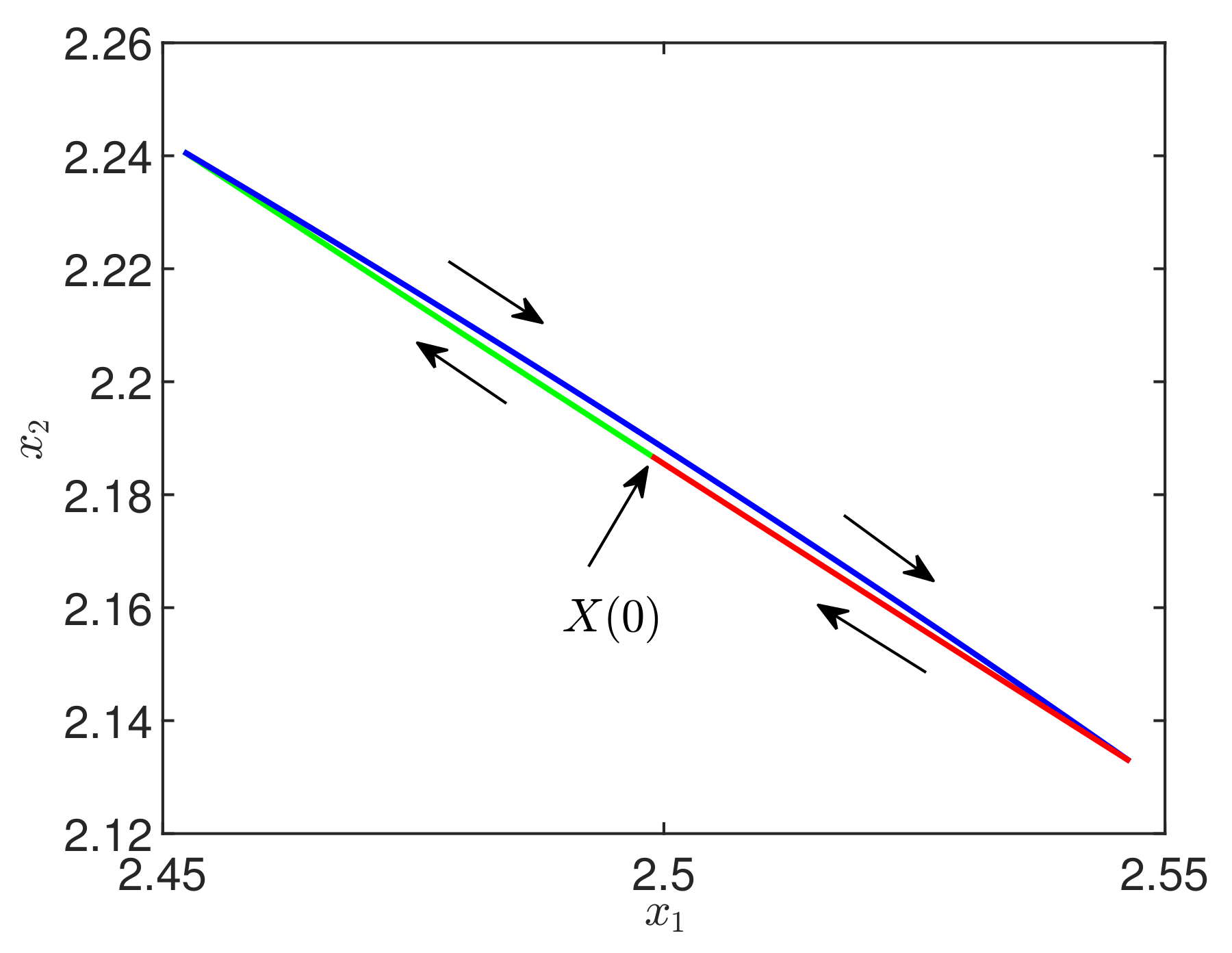
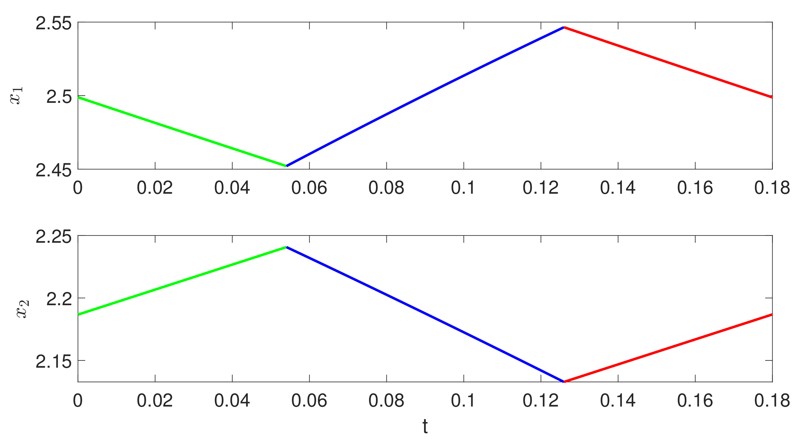
Next, a sufficient condition for the existence of $nT$-periodic orbits is determined. The idea is to successfully apply Equation (26) and use the multiplication theorem for Jacobian determinants [27].

For convenience, the initial condition ${\mathbf{x}}_1$ and the final condition ${\mathbf{x}}_n$ are selected. The duty cycle in the interval $\left[nT,(n+1)T\right]$ is denoted by $d_n$. In addition, $\Sigma$ is the state space of the system (which is the same at each switching instant of the converter).

If $\Sigma \stackrel{P_{n-1}}{\to }\Sigma$ corresponds to the Poincaré application given by Equation (26), then the following expression is defined:

$$\Sigma \stackrel{P_1}{\to }\Sigma \stackrel{P_2}{\to }\Sigma \cdots \Sigma \stackrel{P_{n-1}}{\to }\Sigma ,$$

(55)

and the Poincaré application P is defined such as $P\left({\mathbf{x}}_1\right)={\mathbf{x}}_n$. Then, it follows that:

$$P=P_{n-1}\circ \cdots \circ P_2\circ P_1.$$

(56)

First, from Equation (26) is determined that:

$$\begin{array}{cc}\hfill {\mathbf{x}}_2& ={\varphi }_1\left(\frac{d_1}{2}\right){\varphi }_2\left(T-d_1\right){\varphi }_1\left(\frac{d_1}{2}\right)·{\mathbf{x}}_1+{\varphi }_1\left(\frac{d_1}{2}\right){\varphi }_2\left(T-d_1\right){\psi }_1\left(\frac{d_1}{2}\right)\hfill \\ \hfill & +{\varphi }_1\left(\frac{d_1}{2}\right){\psi }_2\left(T-d_1\right)+{\psi }_1\left(\frac{d_1}{2}\right).\hfill \end{array}$$

(57)

Now, applying the equality of Equation (56), it presents $n\ge 2$:

$${\mathbf{x}}_n=\left[\prod _{i=1}^{n-1}{\varphi }_1\left(\frac{d_i}{2}\right){\varphi }_2\left(T-d_i\right){\varphi }_1\left(\frac{d_i}{2}\right)\right]{\mathbf{x}}_1+{\mathbf{H}}_n,$$

(58)

where the matrix ${\mathbf{H}}_n$ is defined recursively, as follows:

$$\begin{array}{cc}{\mathbf{H}}_1\hfill & ={\varphi }_1\left(\frac{d_1}{2}\right){\varphi }_2\left(T-d_1\right){\psi }_1\left(\frac{d_1}{2}\right)+{\varphi }_1\left(\frac{d_1}{2}\right){\psi }_2\left(T-d_1\right)+{\psi }_1\left(\frac{d_1}{2}\right),\hfill \end{array}$$

(59)

$$\begin{array}{cc}\hfill {\mathbf{H}}_n& ={\varphi }_1\left(\frac{d_n}{2}\right){\varphi }_2\left(T-d_n\right){\varphi }_1\left(\frac{d_n}{2}\right)·{\mathbf{H}}_{n-1}+{\varphi }_1\left(\frac{d_n}{2}\right){\varphi }_2\left(T-d_n\right){\psi }_1\left(\frac{d_n}{2}\right)\hfill \\ \hfill & +{\varphi }_1\left(\frac{d_n}{2}\right){\psi }_2\left(T-d_n\right)+{\psi }_1\left(\frac{d_n}{2}\right).\hfill \end{array}$$

(60)

By considering ${\mathbf{x}}_n={\mathbf{x}}_1$, the following condition for the existence of $nT$-periodic orbits is obtained:

$${\mathbf{x}}_1={\left({\mathbf{I}}_2-\varphi \left(\mathbf{d}\right)\right)}^{-1}·{\mathbf{H}}_n,$$

(61)

where

$$\varphi \left(\mathbf{d}\right)=\prod _{i=1}^{n-1}{\varphi }_1\left(\frac{d_i}{2}\right){\varphi }_2\left(T-d_i\right){\varphi }_1\left(\frac{d_i}{2}\right).$$

(62)

If the spectral radius of the matrix ${\varphi }_1\left(d\right)$ is less than 1, Equation (61) can be applied to guarantee that the system has $nT$-periodic orbits.

Stability of $nT$-Periodic Orbits

The stability of the $nT$-periodic orbits is carried out by considering Equations (47) and (56). Then, from Equation (56):

$$\mathbf{JP}={\mathbf{JP}}_{n-1}\cdots {\mathbf{JP}}_2·{\mathbf{JP}}_1.$$

(63)

Now, from Equation (47), the new expression presented in Equation (64) is obtained:

$${\mathbf{JP}}_j=\frac{\partial {\mathbf{P}}_j}{\partial {\mathbf{x}}_j}+\frac{\partial {\mathbf{P}}_j}{\partial d_j}·\frac{\partial d_j}{\partial {\mathbf{x}}_j}.$$

(64)

Finally, using Equations (63) and (64), and the matrix multiplication by blocks, the new expression obtained is:

$$\mathbf{JP}=\prod _{i=1}^{n-1}\left(\frac{\partial {\mathbf{P}}_{n-i}}{\partial {\mathbf{x}}_{n-i}}\frac{\partial {\mathbf{P}}_{n-i}}{\partial d_{n-i}}\right)\left(\begin{array}{c}{\mathbf{I}}_2\\ {\displaystyle \frac{\partial d_{n-i}}{\partial {\mathbf{x}}_{n-i}}}\end{array}\right).$$

(65)

Therefore, the eigenvalues of the Jacobian matrix given in Equation (65) are calculated to analyze the stability of the $nT$ periodic orbits.

2.8. Floquet Exponents

In this section, the Floquet exponents of the system are obtained, solving the respective equation. In general, this method allows the stability analysis of any periodic orbit; however, the paper focuses on studying $1T$-periodic orbits. The idea is to take a periodic solution of the system ${\mathbf{x}}^{*}$ and perform a perturbation with a time function $e^{\mu t}$. In terms of the unit step function $\theta \left(t\right)$, the system of Equation (6) can be expressed as follows:

$$\begin{array}{cc}\hfill \left(\begin{array}{c}{\dot{x}}_1\\ {\dot{x}}_2\end{array}\right)& =\left(\begin{array}{cc}-\gamma & 0\\ 0& 0\end{array}\right)\left(\begin{array}{c}{x}_1\\ x_2\end{array}\right)+\left(\begin{array}{c}0\\ 1\end{array}\right)+\left(\begin{array}{cc}0& 1\\ -1& 0\end{array}\right)\left(\begin{array}{c}{x}_1\\ x_2\end{array}\right)·\theta \left(t-\frac{d}{2}\right)\hfill \\ \hfill & +\left(\begin{array}{cc}0& -1\\ 1& 0\end{array}\right)\left(\begin{array}{c}{x}_1\\ x_2\end{array}\right)·\theta \left(t-\left(T-\frac{d}{2}\right)\right).\hfill \end{array}$$

(66)

With

$$\left(\begin{array}{c}{x}_1\\ x_2\end{array}\right)=\left(\begin{array}{c}{x}_1^{*}+e^{\mu t}a\\ x_2^{*}+e^{\mu t}b\end{array}\right),$$

(67)

a periodic orbit perturbation ${\left(x_1^{*}{x}_2^{*}\right)}^T$, where a and b are time functions t.

Thus, applying this perturbation to the system of Equation (66), the obtained expression is:

$$\begin{array}{cc}\hfill \left(\begin{array}{c}{\dot{x}}_1^{*}+\mu e^{\mu t}a+e^{\mu t}\dot{a}\\ {\dot{x}}_2^{*}+\mu e^{\mu t}b+e^{\mu t}\dot{b}\end{array}\right)& =\left(\begin{array}{cc}-\gamma & 0\\ 0& 0\end{array}\right)\left(\begin{array}{c}{x}_1^{*}+e^{\mu t}a\\ x_2^{*}+e^{\mu t}b\end{array}\right)+\left(\begin{array}{c}0\\ 1\end{array}\right)\hfill \\ \hfill & +\left(\begin{array}{cc}0& 1\\ -1& 0\end{array}\right)\left(\begin{array}{c}{x}_1^{*}+e^{\mu t}a\\ x_2^{*}+e^{\mu t}b\end{array}\right)·\theta \left(t-\frac{d}{2}\right)\hfill \\ \hfill & +\left(\begin{array}{cc}0& -1\\ 1& 0\end{array}\right)\left(\begin{array}{c}{x}_1^{*}+e^{\mu t}a\\ x_2^{*}+e^{\mu t}b\end{array}\right)·\theta \left(t-\left(T-\frac{d}{2}\right)\right).\hfill \end{array}$$

The duty cycle d is calculated from Equation (20) and can be expressed as:

$$d={\displaystyle \frac{(2k_1-\gamma T{k}_1-k_{2}T)x_1+(2k_2+k_{1}T)x_2+(k_{2}T-2k_1{x}_{1ref}-2k_2{x}_{2ref})}{k_1{x}_2-k_2{x}_1}}.$$

(68)

Now, $d=d(x_1,x_2)$. Then, after linearizing d around the point $X\left(0\right)={(x_1\left(0\right),x_2\left(0\right))}^T$ the following expression is obtained:

$$d=d(x_1,x_2)\approx d(x_1\left(0\right),x_2\left(0\right))+{\left.\frac{\partial d}{\partial x_1}\right|}_{X\left(0\right)}\left(x_1-x_1\left(0\right)\right)+{\left.\frac{\partial d}{\partial x_2}\right|}_{X\left(0\right)}\left(x_2-x_2\left(0\right)\right).$$

(69)

After simplifying the expression, the following term is obtained:

$$\frac{d}{2}(x_1,x_2)\approx \widetilde{c_1}+\widetilde{c_2}\left(x_1-x_1\left(0\right)\right)+\widetilde{c_3}\left(x_2-x_2\left(0\right)\right).$$

(70)

Therefore,

$$\theta \left(t-{\displaystyle \frac{d^{*}}{2}}\right)\approx \theta \left(t-\left(\widetilde{c_1}+\widetilde{c_2}\left(x_1^{*}\left(0\right)-x_1\left(0\right)\right)+\widetilde{c_3}\left(x_2^{*}\left(0\right)-x_2\left(0\right)\right)\right)\right),$$

(71)

and

$$\theta \left(t-{\displaystyle \frac{d}{2}}\right)\approx \theta \left(t-\left(\widetilde{c_1}+\widetilde{c_2}\left(x_1^{*}\left(0\right)+a\left(0\right)-x_1\left(0\right)\right)+\widetilde{c_3}\left(x_2^{*}\left(0\right)+b\left(0\right)-x_2\left(0\right)\right)\right)\right),$$

(72)

where $d^{*}$ is the duty cycle of the periodic solution $x^{*}$, and d is the duty cycle of the perturbation of said periodic orbit. Approximating by first-order Taylor series expansion, then:

$$\theta \left(t-{\displaystyle \frac{d}{2}}\right)\approx \theta \left(t-{\displaystyle \frac{d^{*}}{2}}\right)+\delta \left(t-{\displaystyle \frac{d^{*}}{2}}\right)\left(\widehat{c_2}a\left(0\right)+\widehat{c_3}b\left(0\right)\right),$$

(73)

where $\widehat{c_2}=\frac{-\widetilde{c_2}}{2}$ and $\widehat{c_3}=\frac{-\widetilde{c_3}}{2}$.

Similarly, by Taylor series expansion for the unit step in $t-\left(T-\frac{d}{2}\right)$:

$$\theta \left(t-\left(T-{\displaystyle \frac{d}{2}}\right)\right)\approx \theta \left(t-\left(T-{\displaystyle \frac{d^{*}}{2}}\right)\right)+\delta \left(t-\left(T-{\displaystyle \frac{d^{*}}{2}}\right)\right)\left(\widehat{c_2}a\left(0\right)+\widehat{c_3}b\left(0\right)\right).$$

(74)

In this way, by substituting in Equation (68), then:

$$\begin{array}{cc}\hfill \left(\begin{array}{c}{\dot{x}}_1^{*}+\mu e^{\mu t}a+e^{\mu t}\dot{a}\\ {\dot{x}}_2^{*}+\mu e^{\mu t}b+e^{\mu t}\dot{b}\end{array}\right)& =\left(\begin{array}{cc}-\gamma & 0\\ 0& 0\end{array}\right)\left(\begin{array}{c}{x}_1^{*}+e^{\mu t}a\\ x_2^{*}+e^{\mu t}b\end{array}\right)+\left(\begin{array}{c}0\\ 1\end{array}\right)\hfill \\ \hfill & +\left(\begin{array}{cc}0& 1\\ -1& 0\end{array}\right)\left(\begin{array}{c}{x}_1^{*}+e^{\mu t}a\\ x_2^{*}+e^{\mu t}b\end{array}\right)·\left[\theta \left(t-\frac{d^{*}}{2}\right)\right.\hfill \\ \hfill & +\left.\delta \left(t-{\displaystyle \frac{d^{*}}{2}}\right)\left(\widehat{c_2}a\left(0\right)+\widehat{c_3}b\left(0\right)\right)\right]\hfill \\ \hfill & +\left(\begin{array}{cc}0& -1\\ 1& 0\end{array}\right)\left(\begin{array}{c}{x}_1^{*}+e^{\mu t}a\\ x_2^{*}+e^{\mu t}b\end{array}\right)·\left[\theta \left(t-\left(T-\frac{d^{*}}{2}\right)\right)\right.\hfill \\ \hfill & +\left.\delta \left(t-\left(T-\frac{d^{*}}{2}\right)\right)\left(\widehat{c_2}a\left(0\right)+\widehat{c_3}b\left(0\right)\right)\right].\hfill \end{array}$$

(75)

As ${\left(x_1^{*},x_2^{*}\right)}^T$ is a solution of the system, then from the last equation it follows that:

$$\begin{array}{cc}\hfill \left(\begin{array}{c}\mu e^{\mu t}a+e^{\mu t}\dot{a}\\ \mu e^{\mu t}b+e^{\mu t}\dot{b}\end{array}\right)& =\left(\begin{array}{cc}-\gamma & 0\\ 0& 0\end{array}\right)\left(\begin{array}{c}{e}^{\mu t}a\\ e^{\mu t}b\end{array}\right)\hfill \\ \hfill & +\left(\begin{array}{cc}0& 1\\ -1& 0\end{array}\right)\left(\begin{array}{c}{x}_1^{*}\\ x_2^{*}\end{array}\right)\delta \left(t-{\displaystyle \frac{d^{*}}{2}}\right)\left(\widehat{c_2}a\left(0\right)+\widehat{c_3}b\left(0\right)\right)\hfill \\ \hfill & +\left(\begin{array}{cc}0& 1\\ -1& 0\end{array}\right)\left(\begin{array}{c}{e}^{\mu t}a\\ e^{\mu t}b\end{array}\right)\left[\theta \left(t-\frac{d^{*}}{2}\right)+\delta \left(t-{\displaystyle \frac{d^{*}}{2}}\right)\left(\widehat{c_2}a\left(0\right)+\widehat{c_3}b\left(0\right)\right)\right]\hfill \\ \hfill & +\left(\begin{array}{cc}0& -1\\ 1& 0\end{array}\right)\left(\begin{array}{c}{x}_1^{*}\\ x_2^{*}\end{array}\right)\delta \left(t-\left(T-\frac{d^{*}}{2}\right)\right)\left(\widehat{c_2}a\left(0\right)+\widehat{c_3}b\left(0\right)\right)\hfill \\ \hfill & +\left(\begin{array}{cc}0& -1\\ 1& 0\end{array}\right)\left(\begin{array}{c}{e}^{\mu t}a\\ e^{\mu t}b\end{array}\right)·\left[\theta \left(t-\left(T-\frac{d^{*}}{2}\right)\right)\right.\hfill \\ \hfill & +\left.\delta \left(t-\left(T-\frac{d^{*}}{2}\right)\right)\left(\widehat{c_2}a\left(0\right)+\widehat{c_3}b\left(0\right)\right)\right].\hfill \end{array}$$

(76)

As the delta function:

$\delta \left(t-\frac{d^{*}}{2}\right)$ only contribute to:

$t=\frac{d^{*}}{2}$, and the matrices

$$\left(\begin{array}{c}{e}^{\mu t}a\\ e^{\mu t}b\end{array}\right)\delta \left(t-{\displaystyle \frac{d^{*}}{2}}\right)\left(\widehat{c_2}a\left(0\right)+\widehat{c_3}b\left(0\right)\right)\approx \left(\begin{array}{c}0\\ 0\end{array}\right),$$

(77)

$$\left(\begin{array}{c}{e}^{\mu t}a\\ e^{\mu t}b\end{array}\right)\delta \left(t-\left(T-{\displaystyle \frac{d^{*}}{2}}\right)\right)\left(\widehat{c_2}a\left(0\right)+\widehat{c_3}b\left(0\right)\right)\approx \left(\begin{array}{c}0\\ 0\end{array}\right),$$

(78)

then the perturbed system can be written as:

$$\begin{array}{cc}\hfill \left(\begin{array}{c}\mu a+\dot{a}\\ \mu b+\dot{b}\end{array}\right)& =\left(\begin{array}{cc}-\gamma & 0\\ 0& 0\end{array}\right)\left(\begin{array}{c}a\\ b\end{array}\right)+\mathbf{A}\delta \left(t-{\displaystyle \frac{d^{*}}{2}}\right)\left(\begin{array}{c}a\left(0\right)\\ b\left(0\right)\end{array}\right)\hfill \\ \hfill & +\left(\begin{array}{cc}0& 1\\ -1& 0\end{array}\right)\left(\begin{array}{c}a\\ b\end{array}\right)\theta \left(t-\frac{d^{*}}{2}\right)\hfill \\ \hfill & +\mathbf{B}\delta \left(t-\left(T-\frac{d^{*}}{2}\right)\right)\left(\begin{array}{c}a\left(0\right)\\ b\left(0\right)\end{array}\right)\hfill \\ \hfill & +\left(\begin{array}{cc}0& -1\\ 1& 0\end{array}\right)\left(\begin{array}{c}a\\ b\end{array}\right)\theta \left(t-\left(T-\frac{d^{*}}{2}\right)\right).\hfill \end{array}$$

(79)

where

$$\mathbf{A}=e^{-\mu \left(\frac{d^{*}}{2}\right)}\left(\begin{array}{cc}0& 1\\ -1& 0\end{array}\right)\left(\begin{array}{c}{x}_1^{*}\left(\frac{d^{*}}{2}\right)\\ x_2^{*}\left(\frac{d^{*}}{2}\right)\end{array}\right)\left(\begin{array}{cc}\widehat{c_2}& \widehat{c_3}\end{array}\right),$$

(80)

and

$$\mathbf{B}=e^{-\mu \left(T-\frac{d^{*}}{2}\right)}\left(\begin{array}{cc}0& -1\\ 1& 0\end{array}\right)\left(\begin{array}{c}{x}_1^{*}\left(T-\frac{d^{*}}{2}\right)\\ x_2^{*}\left(T-\frac{d^{*}}{2}\right)\end{array}\right)\left(\begin{array}{cc}\widehat{c_2}& \widehat{c_3}\end{array}\right).$$

(81)

The expression is obtained:

$$\left(\begin{array}{c}{x}_1^{*}\left(\frac{d^{*}}{2}\right)\\ x_2^{*}\left(\frac{d^{*}}{2}\right)\end{array}\right)=e^{A_1\frac{d^{*}}{2}}\left(\begin{array}{c}{x}_1^{*}\left(0\right)\\ x_2^{*}\left(0\right)\end{array}\right)+\frac{d^{*}}{2}B.$$

(82)

and

$$\left(\begin{array}{c}{x}_1^{*}\left(T-\frac{d^{*}}{2}\right)\\ x_2^{*}\left(T-\frac{d^{*}}{2}\right)\end{array}\right)=e^{A_2\left(T-d^{*}\right)}\left(\begin{array}{c}{x}_1^{*}\left(\frac{d^{*}}{2}\right)\\ x_2^{*}\left(\frac{d^{*}}{2}\right)\end{array}\right)+A_2^{-1}\left(e^{A_2\left(T-d^{*}\right)}-{\mathbf{I}}_2\right)B.$$

(83)

It is finally arrived at that the variational equation that governs the evolution of the disturbance is given by:

$$\begin{array}{cc}\hfill \left(\begin{array}{c}\hfill \dot{a}\\ \dot{b}\end{array}\right)& =\left(\begin{array}{cc}-\gamma -\mu & 0\\ 0& -\mu \end{array}\right)\left(\begin{array}{c}a\\ b\end{array}\right)+\mathbf{A}\delta \left(t-{\displaystyle \frac{d}{2}}\right)\left(\begin{array}{c}a\left(0\right)\\ b\left(0\right)\end{array}\right)\hfill \end{array}$$

(84)

$$\begin{array}{cc}\hfill & +\left(\begin{array}{cc}0& 1\\ -1& 0\end{array}\right)\left(\begin{array}{c}a\\ b\end{array}\right)\theta \left(t-\frac{d}{2}\right)\hfill \end{array}$$

(85)

$$\begin{array}{cc}\hfill & +\mathbf{B}\delta \left(t-\left(T-\frac{d}{2}\right)\right)\left(\begin{array}{c}a\left(0\right)\\ b\left(0\right)\end{array}\right)\hfill \end{array}$$

(86)

$$\begin{array}{cc}\hfill & +\left(\begin{array}{cc}0& -1\\ 1& 0\end{array}\right)\left(\begin{array}{c}a\\ b\end{array}\right)\theta \left(t-\left(T-\frac{d}{2}\right)\right).\hfill \end{array}$$

(87)

where $d^{*}=d$ is obtained simply for convenience. The next step is to solve this variational equation. The integrals of the perturbation equations must be done piecewise, and due to the presence of the function Dirac delta, integration over discontinuities is also required. Initially, a solution between $t=0$ and $t=\frac{d}{2}$ is obtained to calculate $a{\left({\displaystyle \frac{d}{2}}\right)}_{-}$ and $b{\left({\displaystyle \frac{d}{2}}\right)}_{-}$.

Now, in $0<t<{\displaystyle \frac{d}{2}}$, the variational equation is converted to:

$$\left(\begin{array}{c}\dot{a}\\ \dot{b}\end{array}\right)=\left(\begin{array}{cc}-\gamma -\mu & 0\\ 0& -\mu \end{array}\right)\left(\begin{array}{c}a\\ b\end{array}\right)$$

(88)

Then, the solution of this system is given by Equation (89).

$$\left(\begin{array}{c}a\\ b\end{array}\right)=e^{-\mu t}\left(\begin{array}{cc}{e}^{-\gamma t}& 0\\ 0& 1\end{array}\right)\left(\begin{array}{c}a\left(0\right)\\ b\left(0\right)\end{array}\right),$$

(89)

and consequently,

$$\left(\begin{array}{c}a{\left(\frac{d}{2}\right)}_{-}\\ b{\left(\frac{d}{2}\right)}_{-}\end{array}\right)=e^{-\mu \frac{d}{2}}\left(\begin{array}{cc}{e}^{-\gamma \frac{d}{2}}& 0\\ 0& 1\end{array}\right)\left(\begin{array}{c}a\left(0\right)\\ b\left(0\right)\end{array}\right).$$

(90)

After integrating over the discontinuity to find $a{\left(\frac{d}{2}\right)}_{+}$ and $b{\left(\frac{d}{2}\right)}_{+}$, we finally obtain Equation (91).

$$\left(\begin{array}{c}a{\left(\frac{d}{2}\right)}_{+}\\ b{\left(\frac{d}{2}\right)}_{+}\end{array}\right)=\left(\begin{array}{c}a{\left(\frac{d}{2}\right)}_{-}\\ b{\left(\frac{d}{2}\right)}_{-}\end{array}\right)+\mathbf{A}\left(\begin{array}{c}a\left(0\right)\\ b\left(0\right)\end{array}\right).$$

(91)

Therefore,

$$\left(\begin{array}{c}a{\left(\frac{d}{2}\right)}_{+}\\ b{\left(\frac{d}{2}\right)}_{+}\end{array}\right)=\left(e^{-\mu \frac{d}{2}}\left(\begin{array}{cc}{e}^{-\gamma \frac{d}{2}}& 0\\ 0& 1\end{array}\right)+\mathbf{A}\right)\left(\begin{array}{c}a\left(0\right)\\ b\left(0\right)\end{array}\right).$$

(92)

Now, after integrating between $t=\frac{d}{2}$ and $t=T-\frac{d}{2}$ with this new initial condition, the expression found is:

$${\left(\begin{array}{cc}a{\left(T-\frac{d}{2}\right)}_{-}& b{\left(T-\frac{d}{2}\right)}_{-}\end{array}\right)}^T.$$

(93)

First, in this interval, the disturbed system is as in Equation (94):

$$\left(\begin{array}{c}\dot{a}\\ \dot{b}\end{array}\right)=\left(\begin{array}{cc}-\gamma -\mu & 1\\ -1& -\mu \end{array}\right)\left(\begin{array}{c}a\\ b\end{array}\right).$$

(94)

It is convenient to express the term C as in Equation (95) to find the solution to this system.

$$\mathbf{C}=\left(\begin{array}{cc}-\gamma -\mu & 1\\ -1& -\mu \end{array}\right).$$

(95)

The mathematical expression in Equation (95) can be simplified by considering that it is a function of $A_1$ and $A_2$, as shown in Equation (96).

$$\mathbf{C}={\mathbf{A}}_1+{\mathbf{A}}_2,$$

(96)

where both terms $A_1$ and $A_2$ are expressed according to the parameter $\gamma$ and $\mu$, as shown in Equations (97) and (98):

$${\mathbf{A}}_1=\left(\begin{array}{cc}-\frac{\gamma }{2}-\mu & 0\\ 0& -\frac{\gamma }{2}-\mu \end{array}\right),$$

(97)

$${\mathbf{A}}_2=\left(\begin{array}{cc}-\frac{\gamma }{2}& 1\\ -1& \frac{\gamma }{2}\end{array}\right).$$

(98)

The advantage of using $A_1$ and $A_2$ is that the expression can be simply expressed as shown in Equation (99).

$$e^{\mathbf{C}t}=e^{{\mathbf{A}}_{1}t}{e}^{{\mathbf{A}}_{2}t},$$

(99)

where

$$e^{{\mathbf{A}}_{1}t}=e^{-\left(\frac{\gamma }{2}+\mu \right)t}{\mathbf{I}}_2,$$

(100)

and

$$e^{{\mathbf{A}}_{2}t}=\left(\begin{array}{cc}-\frac{\gamma }{\sqrt{\alpha }}sin\left(\frac{1}{2}\sqrt{\alpha }t\right)+cos\left(\frac{1}{2}\sqrt{\alpha }t\right)& \frac{2}{\sqrt{\alpha }}sin\left(\frac{1}{2}\sqrt{\alpha }t\right)\\ -\frac{2}{\sqrt{\alpha }}sin\left(\frac{1}{2}\sqrt{\alpha }t\right)& \frac{\gamma }{\sqrt{\alpha }}sin\left(\frac{1}{2}\sqrt{\alpha }t\right)+cos\left(\frac{1}{2}\sqrt{\alpha }t\right)\end{array}\right),$$

(101)

with $\alpha =4-{\gamma }^2$. In consequence,

$$\left(\begin{array}{c}a{\left(T-\frac{d}{2}\right)}_{-}\\ b{\left(T-\frac{d}{2}\right)}_{-}\end{array}\right)=e^{-(\frac{\gamma }{2}+\mu )(T-\frac{d}{2})}{e}^{{\mathbf{A}}_2(T-\frac{d}{2})}\left(\begin{array}{c}a{\left(\frac{d}{2}\right)}_{+}\\ b{\left(\frac{d}{2}\right)}_{+}\end{array}\right).$$

(102)

By replacing the matrix $\left(\begin{array}{c}a{\left(\frac{d}{2}\right)}_{+}\\ b{\left(\frac{d}{2}\right)}_{+}\end{array}\right)$ the expression obtained is that presented in (103).

$$\left(\begin{array}{c}a{\left(T-\frac{d}{2}\right)}_{-}\\ b{\left(T-\frac{d}{2}\right)}_{-}\end{array}\right)=e^{-(\frac{\gamma }{2}+\mu )(T-\frac{d}{2})}{e}^{{\mathbf{A}}_2(T-\frac{d}{2})}\left(e^{-\mu \frac{d}{2}}\left(\begin{array}{cc}{e}^{-\gamma \frac{d}{2}}& 0\\ 0& 1\end{array}\right)+\mathbf{A}\right)\left(\begin{array}{c}a\left(0\right)\\ b\left(0\right)\end{array}\right).$$

(103)

Now, we integrate over the second discontinuity to find the state at $t={(T-\frac{d}{2})}_{+}$:

$$\begin{array}{cc}\hfill \left(\begin{array}{c}a{\left(T-\frac{d}{2}\right)}_{+}\\ b{\left(T-\frac{d}{2}\right)}_{+}\end{array}\right)& =e^{-(\frac{\gamma }{2}+\mu )(T-\frac{d}{2})}{e}^{{\mathbf{A}}_2(T-\frac{d}{2})}\left(e^{-\mu \frac{d}{2}}\left(\begin{array}{cc}{e}^{-\gamma \frac{d}{2}}& 0\\ 0& 1\end{array}\right)+\mathbf{A}\right)\left(\begin{array}{c}a\left(0\right)\\ b\left(0\right)\end{array}\right)\hfill \\ \hfill & +\mathbf{B}\left(\begin{array}{c}a\left(0\right)\\ b\left(0\right)\end{array}\right).\hfill \end{array}$$

(104)

In order to simplify the expression:

$$\mathbf{H}=e^{-(\frac{\gamma }{2}+\mu )(T-\frac{d}{2})}{e}^{{\mathbf{A}}_2(T-\frac{d}{2})}\left(e^{-\mu \frac{d}{2}}\left(\begin{array}{cc}{e}^{-\gamma \frac{d}{2}}& 0\\ 0& 1\end{array}\right)+\mathbf{A}\right).$$

(105)

Now, $a\left(T\right)$ and $b\left(T\right)$ are calculated, integrating over the last section:

$$\left(\begin{array}{c}a\left(T\right)\\ b\left(T\right)\end{array}\right)=e^{-\mu \frac{d}{2}}\left(\begin{array}{cc}{e}^{-\gamma \frac{d}{2}}& 0\\ 0& 1\end{array}\right)\left(\begin{array}{c}a{\left(T-\frac{d}{2}\right)}_{+}\\ b{\left(T-\frac{d}{2}\right)}_{+}\end{array}\right).$$

(106)

Therefore,

$$\left(\begin{array}{c}a\left(T\right)\\ b\left(T\right)\end{array}\right)=e^{-\mu \frac{d}{2}}\left(\begin{array}{cc}{e}^{-\gamma \frac{d}{2}}& 0\\ 0& 1\end{array}\right)\left(\mathbf{H}+\mathbf{B}\right)\left(\begin{array}{c}a\left(0\right)\\ b\left(0\right)\end{array}\right).$$

(107)

Then, if the last equation is written as:

$$\left(\begin{array}{c}a\left(T\right)\\ b\left(T\right)\end{array}\right)={\mathbf{A}}_p\left(\begin{array}{c}a\left(0\right)\\ b\left(0\right)\end{array}\right).$$

(108)

Since the 1T-periodic orbits are determined, then $a\left(T\right)=a\left(0\right)$ and $b\left(T\right)=b\left(0\right)$ are considered.

$$\left({\mathbf{A}}_p-{\mathbf{I}}_2\right)\left(\begin{array}{c}a\left(0\right)\\ b\left(0\right)\end{array}\right)=\left(\begin{array}{c}0\\ 0\end{array}\right).$$

(109)

This solution is stable if the real part of the Floquet exponents $\mu$, obtained from the solution of the variational equation, is negative. This would be comply if $\mu <0$ considering that $det\left({\mathbf{A}}_p-{\mathbf{I}}_2\right)=0$.

3. Results and Discussion

In this section, the stability of periodic orbits is analyzed. In addition, the spectral radius of the Jacobian matrix is used to determine the stability limits of the periodic orbits.

3.1. Stability of Periodic Orbits

Figure 2 shows the variation of the spectral radius of the matrix given in Equation (30). According to Equation (29) and with the parameters $\gamma \in (0.3,0.5)$ and $T=0.18$, the system presents 1T-periodic orbits.

Figure 3 shows a 1T-periodic orbit in the state space. The green line corresponds to the evolution of the orbit for the $1N$ configuration (first switching). The blue line corresponds to the evolution of the orbit for the configuration that considers the switch OFF. Finally, the red line corresponds to the last configuration with the switch ON.

Figure 4 represents the evolution of the current ($x_1$) and the voltage ($x_2$) in a commutation period. Similar to the previous figure, each color represents the orbit evolution for each configuration: green is for $1N$, blue is for OFF, and red is for ON. In a possible experimental test, seeking the steady-state operation, it is expected that the evolution of the system will tend to the limit cycle and to a point close to the desired reference value for the controlled signal $x_2$. When the controller stops working correctly, the behavior is no longer a limit cycle, but subharmonics of higher order periods appear, which lead to lower frequency signals and, finally, chaos can occur. It should be noted that in an experimental test, an ideal limit cycle is impossible because of the electronic noise that is always present in the voltage and current signals [9,28].

When implementing a boost converter, it is necessary to keep in mind the evolution of the voltage $x_2$, as this generally must have low ripple and a regulation error of less than 3%. The ZAD technique is used to control the output signal $x_2$, and this signal gets close to the reference signal defined by the user, as shown in Figure 4.

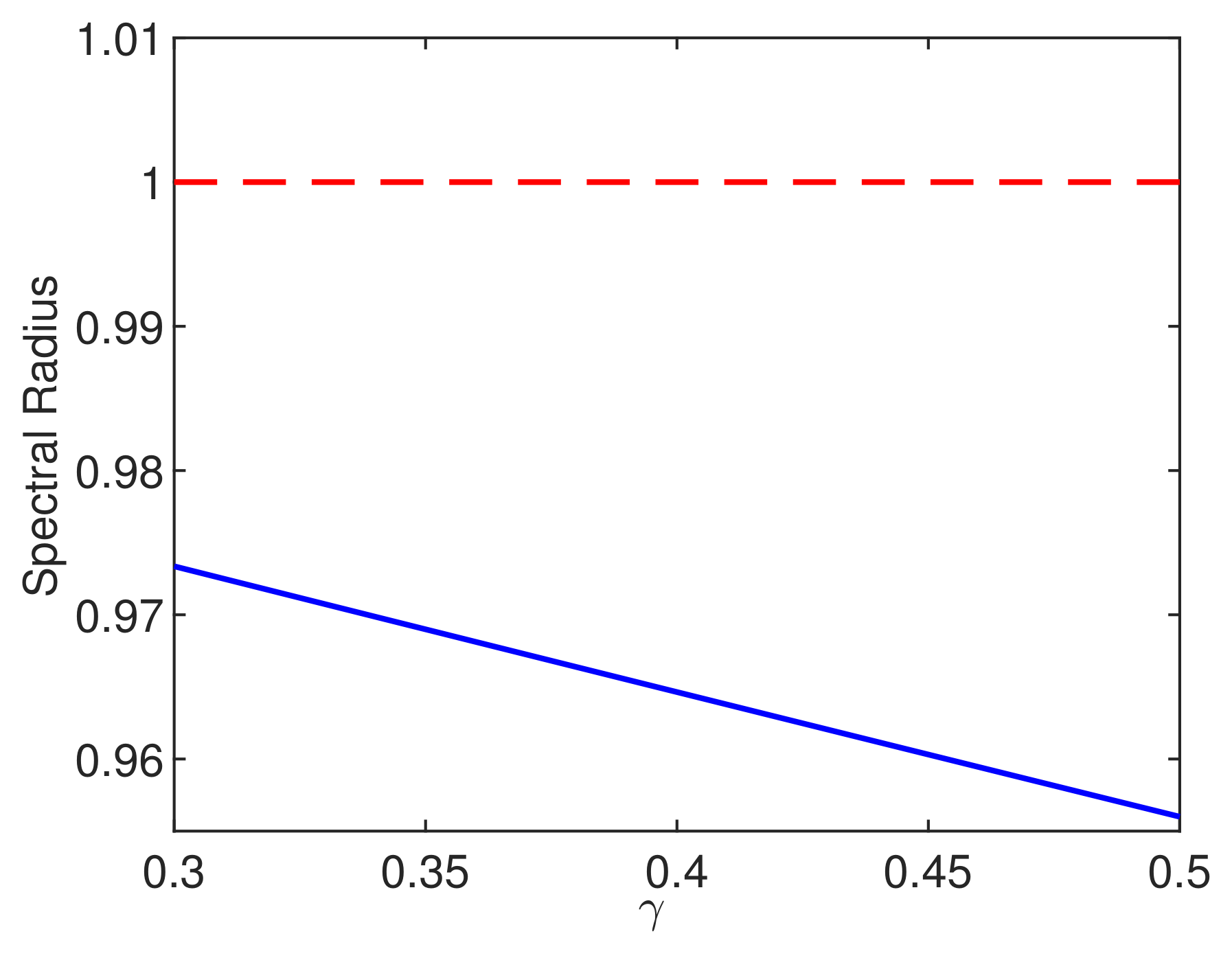
3.2. Spectral Radius of the Jacobian Matrix

Next, the variation of the spectral radius of the Jacobian matrix in the Poincaré application (Equation (47)) is evaluated at the equilibrium points given by Equation (29) (see Figure 5).

In this figure, $T=0.18$, $k_2=0.5$, and $\gamma =0.35$ have been chosen. As the spectral radius values move from less than 1 to greater than 1 just at $k_1=-0.26$, there is a stability change in the $1T$-periodic orbit. Then, for $k_1=-0.26$, the system presents a bifurcation point.

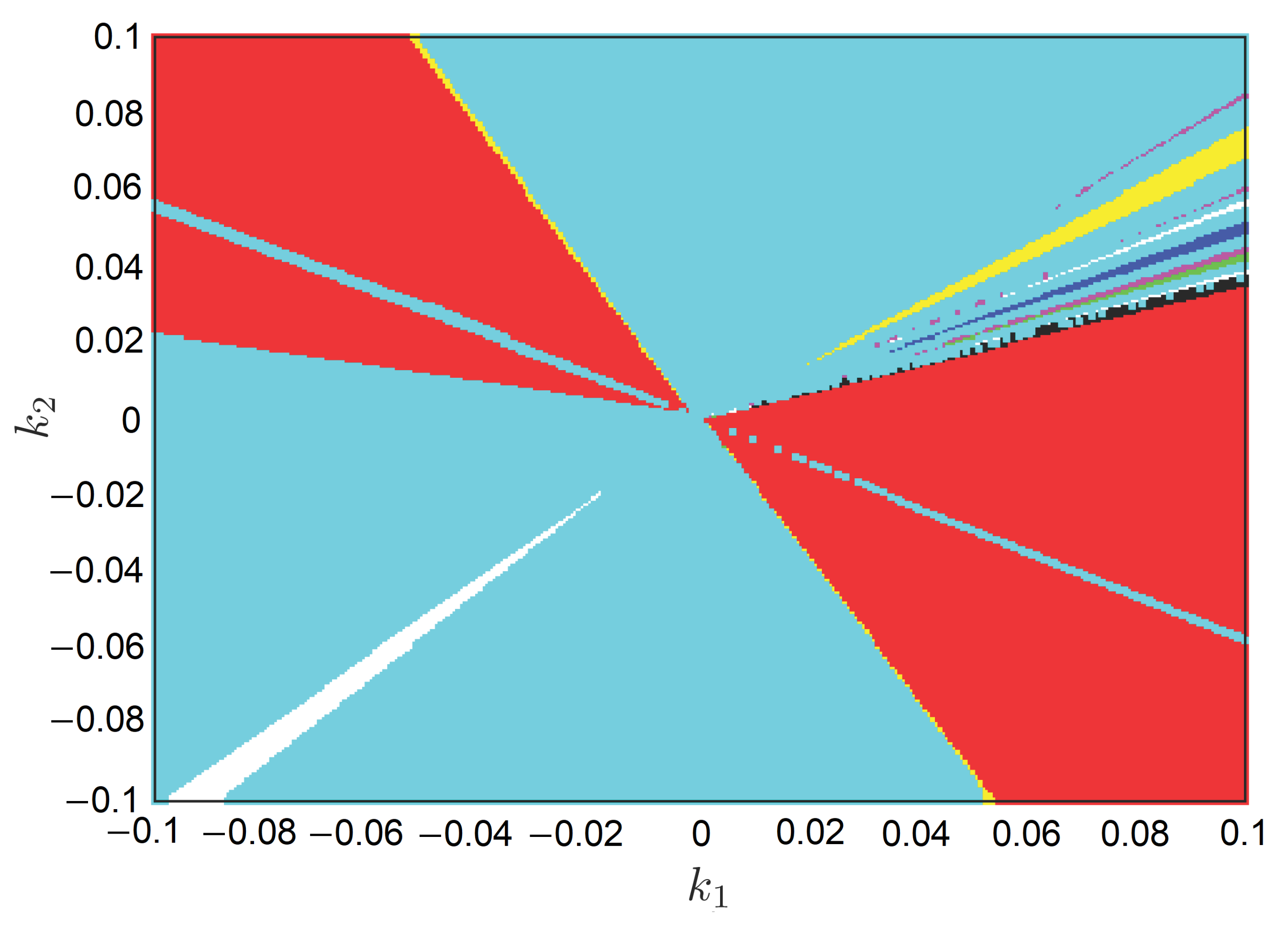
3.3. Biparametric Diagram

Figure 6 shows a biparametric diagram with $k_1$ on the abscissa axis and $k_2$ on the ordinate axis. This figure helps identify stability from $1T-$ to $7T$-periodic orbits. For this figure, the same initial conditions ${\left(2.52.1875\right)}^T$, $\gamma =0.35$, and $T=0.18$ seg are considered. In this plot, red corresponds to areas with $1T$-periodic orbits, yellow to $2T$-periodic orbits, blue to $3T$-periodic orbits, green to $4T$-periodic orbits, white to $5T$-periodic orbits, black to $6T$-periodic orbits, magenta to $7T$-periodic orbits, and cyan to higher orbits.

Regarding Figure 6, in an experimental test, it is desired that the vast majority of points in the biparametric diagram belong to $1T$-periodic orbits (red point), which represent stability in the controlled system. It is desired that 1T-periodic orbits have the same frequency as the switch (MOSFET). This ensures that chattering is eliminated in the system, subharmonics are reduced, and the system is more stable. In this paper, the ZAD technique is used to control the voltage, but the user must give it the values of $k_1$ and $k_2$ in such a way that the system evolves to $1T$-periodic orbits. The biparametric diagram of Figure 6 shows the $k_1$ and $k_2$ values to obtain stability.

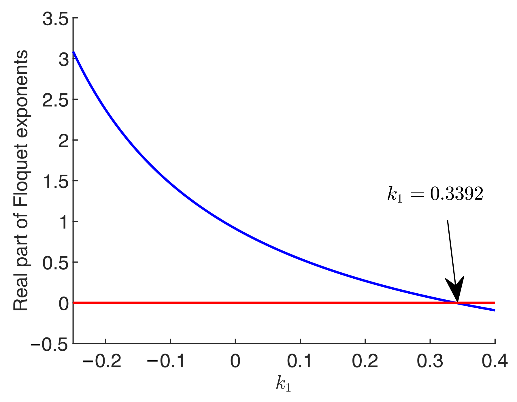
3.4. Floquet Exponents

Equation (109) allows simulating the real component of the Floquet exponents associated with the $1T$-periodic orbit. In Figure 7, $k_2=-0.5$, $\gamma =0.35$, and $T=0.18$ are selected. This result shows that for $K_1>0.3392$, the 1T-periodic orbit is stable. A formula was found that gives sufficient conditions for the existence of $nT$ periodic orbits (Equation (61)) and their respective stability (Equation (65)).

4. Conclusions

This paper presented the analysis of the existence of $nT$-periodic orbits in the boost converter. The stability of these orbits is evaluated via the eigenvalues of the Jacobian matrix of the Poincaré application. A wide range of the $\gamma$ parameter was determined, and the detection of $1T$-periodic orbits was made. A particular class of $2T$-periodic orbits was studied in the boost converter, and a closed formula was found with a sufficient condition for the existence of $nT$-periodic orbits and stability. An analytical calculation of the Floquet exponents was performed to determine the stability limit of the $1T$-periodic orbit.

In a possible experimental test seeking the steady-state operation, it is expected that the evolution of the system will tend to a point close to the desired reference value for the controlled signal $x_2$. When the control is not working correctly, the limit cycle is of larger size and sub harmonics of $nT$-periodic orbits appear, which leads to lower frequency signals and finally chaos. It is desired that the vast majority of points in the biparametric diagram belong to $1T$-periodic orbits, which represent stability in the controlled system. In this paper, the ZAD technique is used to control the voltage, but the user must give it the values of $k_1$ and $k_2$ in such a way the system evolves to $1T$-periodic orbits.

References

1. Blaabjerg, F.; Chen, Z.; Kjaer, S. Power electronics as efficient interface in dispersed power generation systems. IEEE Trans. Power Electron. 2004, 19, 1184–1194. [Google Scholar] [CrossRef]
2. Farh, H.; Othman, M.; Eltamaly, A.; Al-Saud, M. Maximum Power Extraction from a Partially Shaded PV System Using an Interleaved Boost Converter. Energies 2018, 11, 2543. [Google Scholar] [CrossRef]
3. Revelo-Fuelagán, J.; Candelo-Becerra, J.E.; Hoyos, F.E. Power Factor Correction of Compact Fluorescent and Tubular LED Lamps by Boost Converter with Hysteretic Control. J. Daylight. 2020, 7, 73–83. [Google Scholar] [CrossRef]
4. Fossas, E.; Olivar, G. Study of chaos in the buck converter. IEEE Trans. Circuits Syst. I Fundam. Theory Appl. 1996, 43, 13–25. [Google Scholar] [CrossRef]
5. Toribio, E.; El Aroudi, A.; Olivar, G.; Benadero, L. Numerical and experimental study of the region of period-one operation of a PWM boost converter. IEEE Trans. Power Electron. 2000, 15, 1163–1171. [Google Scholar] [CrossRef]
6. Poddar, G.; Chakrabarty, K.; Banerjee, S. Experimental control of chaotic behavior of buck converter. IEEE Trans. Circuits Syst. I Fundam. Theory Appl. 1995, 42, 502–504. [Google Scholar] [CrossRef]
7. Di Bernardo, M.; Garefalo, F.; Glielmo, L.; Vasca, F. Switchings, bifurcations, and chaos in DC/DC converters. IEEE Trans. Circuits Syst. I Fundam. Theory Appl. 1998, 45, 133–141. [Google Scholar] [CrossRef]
8. Repecho, V.; Biel, D.; Ramos-Lara, R. Robust ZAD Sliding Mode Control for an 8-Phase Step-Down Converter. IEEE Trans. Power Electron. 2020, 35, 2222–2232. [Google Scholar] [CrossRef]
9. Vergara Perez, D.D.C.; Trujillo, S.C.; Hoyos Velasco, F.E. Period Addition Phenomenon and Chaos Control in a ZAD Controlled Boost Converter. Int. J. Bifurc. Chaos 2018, 28, 1850157. [Google Scholar] [CrossRef]
10. Repecho, V.; Biel, D.; Ramos-Lara, R.; Vega, P.G. Fixed-Switching Frequency Interleaved Sliding Mode Eight-Phase Synchronous Buck Converter. IEEE Trans. Power Electron. 2018, 33, 676–688. [Google Scholar] [CrossRef] [Green Version]
11. Chatterjee, K.; Ghosh, A.; Saha, P.K.; Das, A. An analysis of power-factor-correction boost converter’s nonlinear dynamics through bifurcation diagrams. In Proceedings of the 2016 International Conference on Intelligent Control Power and Instrumentation (ICICPI), Kolkata, India, 21–23 October 2016; pp. 142–147. [Google Scholar] [CrossRef]
12. Angulo, F.; Fossas, E.; Olivar, G. Transition from Periodicity to Chaos in a PWM-Controlled Buck Converter with ZAD Strategy. Int. J. Bifurc. Chaos 2005, 15, 3245–3264. [Google Scholar] [CrossRef]
13. Trujillo, S.C.; Candelo-Becerra, J.E.; Hoyos, F.E. Numerical Validation of a Boost Converter Controlled by a Quasi-Sliding Mode Control Technique with Bifurcation Diagrams. Symmetry 2022, 14, 694. [Google Scholar] [CrossRef]
14. Munoz, J.; Osorio, G.; Angulo, F. Boost converter control with ZAD for power factor correction based on FPGA. In Proceedings of the 2013 Workshop on Power Electronics and Power Quality Applications (PEPQA), Bogota, Colombia, 6–7 July 2013; pp. 1–5. [Google Scholar] [CrossRef]
15. El Aroudi, A.; Orabi, M. Stabilizing Technique for AC–DC Boost PFC Converter Based on Time Delay Feedback. IEEE Trans. Circuits Syst. II Express Briefs 2010, 57, 56–60. [Google Scholar] [CrossRef]
16. Aroudi, A.E.; Debbat, M.; Martinez-Salamero, L. Poincaré maps modeling and local orbital stability analysis of discontinuous piecewise affine periodically driven systems. Nonlinear Dyn. 2007, 50, 431–445. [Google Scholar] [CrossRef]
17. Amador, A.; Casanova, S.; Granada, H.A.; Olivar, G.; Hurtado, J. Codimension-Two Big-Bang Bifurcation in a ZAD-Controlled Boost DC-DC Converter. Int. J. Bifurc. Chaos 2014, 24, 1450150. [Google Scholar] [CrossRef]
18. Baumeister, J.; Leitao, A. Introdução à Teoria de Controle e Programação Dinâmica; Instituto de Matemática Pura e Aplicada: Rio de Janeiro, Brazil, 2014; p. 399. [Google Scholar]
19. Doering, C.I.; Lopes, A.O. Equacoes Diferenciais Ordinárias; Instituto de Matemática Pura e Aplicada: Rio de Janeiro, Brazil, 2016; p. 423. [Google Scholar]
20. Fossas, E.; Griñó, R.; Biel, D. Quasi-sliding control based on pulse width modulation, zero dynamics and the L2 norm. In Proceedings of the Advances in Variable Structure Systems; WORLD SCIENTIFIC: Singapore, 2000; pp. 335–344. [Google Scholar] [CrossRef]
21. Hoyos, F.E.; Candelo-Becerra, J.E.; Hoyos Velasco, C.I. Model-Based Quasi-Sliding Mode Control with Loss Estimation Applied to DC–DC Power Converters. Electronics 2019, 8, 1086. [Google Scholar] [CrossRef]
22. Kuznetsov, Y.A. Elements of Applied Bifurcation Theory, 3rd ed.; Springer: New York, NY, USA, 2004; Volume 112, p. 634. [Google Scholar] [CrossRef]
23. Parker, T.S.; Chua, L.O. Practical Numerical Algorithms for Chaotic Systems, 1st ed.; Springer: New York, NY, USA, 1989; p. 348. [Google Scholar] [CrossRef]
24. Devaney, R.L. An Introduction to Chaotic Dynamical Systems, 3rd ed.; Chapman and Hall/CRC: Boca Raton, FL, USA, 2021; pp. 1–432. [Google Scholar] [CrossRef]
25. Nieto, J.I. Introducción a los espacios de Hilbert; Programa Regional de Desarrollo Científico y Tecnológico, Departamento de Asuntos Científicos, Secretaría General de la Organización de los Estados Americanos: Washington, DC, USA, 1978; p. 150. [Google Scholar]
26. Bachman, G.; Narici, L. Functional Analysis; Dover Publications: Mineola, NY, USA, 2000; p. 532. [Google Scholar]
27. Munkres, J.R. Analysis on Manifolds, 1st ed.; Addison-Wesley Publishing Company: Redwood City, CA, USA, 1991; p. 366. [Google Scholar]
28. Hoyos Velasco, F.E.; García, N.T.; Garcés Gómez, Y.A. Adaptive Control for Buck Power Converter Using Fixed Point Inducting Control and Zero Average Dynamics Strategies. Int. J. Bifurc. Chaos 2015, 25, 1550049. [Google Scholar] [CrossRef]
Figure 1. Diagram of the boost converter.
Applsci 12 09565 g001
Figure 2. Variation of the spectral radius as a function of γ .
Applsci 12 09565 g002
Figure 3. A 1T-periodic orbit.
Applsci 12 09565 g003
Figure 4. Evolution of voltage and current.
Applsci 12 09565 g004
Figure 5. Spectral radius as a function of k 1 to determine the stability limit of 1T-periodic orbits.
Applsci 12 09565 g005
Figure 6. Existence of stable orbits.
Applsci 12 09565 g006
Figure 7. Floquet exponents with PWMC.
Applsci 12 09565 g007
Publisher’s Note: MDPI stays neutral with regard to jurisdictional claims in published maps and institutional affiliations.