An Energy Aware Grid-Based Clustering Power Efficient Data Aggregation Protocol for Wireless Sensor Networks

Abstract

A wireless sensor network (WSN) is made up of multiple sensors deployed in a specific sensing area to identify the occurrence of events and quickly transmit useful information back to the base station (BS). In WSNs, schemes to reduce energy consumption are an important topic of research. A well-designed data transmission scheme can effectively extend the lifetime of a network. In this paper, we propose an energy aware grid-based clustering power efficient data aggregation protocol (GB-PEDAP) for WSNs. The proposed scheme has a two-layer architecture: the inner layer and the outer layer. The inner layer uses direct transmission to collect the data of the cluster (cell), and the outer layer uses a tree structure transmission to collect the data of the cluster head (cell head). In our simulations, the number of rounds executed by GB-PEDAP was approximately 1.2 rounds of TBEEP, 1.3 rounds of GSTEB, and 1.5 rounds of PEDAP. With the initial energy, 0.25 J, the execution rounds of the first node death for GB-PEDAP, TBEEP, GSTEB, and PEDAP were 751, 572, 486, and 339, respectively. The proposed GB-PEDAP can evenly disperse the energy consumption of sensors to avoid the rapid death of sensors, extending the lifetime of a WSN.

1. Introduction

Due to the vigorous development of wireless networks and the Internet of Things (IoTs), the technology and application of wireless sensor networks (WSNs) has become increasingly important. WSNs use sensors deployed in a specific area to detect changes in the surrounding environment. After detecting the data of interest, sensors transmit the detected data to the base station (BS) by wireless transmission [1,2,3]. Therefore, WSNs can be widely applied in various fields, such as traffic monitoring, agricultural application, and industrial control [4,5,6].

In WSNs, sensors mainly detect environmental changes, and then send the detected data to the BS by direct or multi-hop transmission through the wireless network. The energy consumption of sensors is based on the energy consumption caused by the transmission and reception of data. Moreover, data aggregation refers to the data collected by the sensors for data compression and fusion [7,8], which is then transmitted to the BS. Data aggregation saves energy by reducing the amount of data and number of data transmissions. Therefore, an energy efficient data aggregation scheme can prolong a network’s lifetime. However, direct transmission schemes consume more energy because of the long transmission distance. Hence, direct transmission is more suitable for sensing environments with a small range.

Sensors have some limitations, such as energy, storage space, and computing capability. The process of receiving and transmitting data consumes a sensor’s energy, which may cause the energy of them to be exhausted and result in their unavailability. It is not easy to recharge the sensors or replace the batteries in a large-scale WSN. Therefore, exploring energy efficient schemes to reduce energy consumption and extend the network lifetime is key to designing data aggregation schemes.

The contributions of the proposed scheme consist of three items. Firstly, a two-layer grid-based data aggregation scheme for WSNs is presented, called the grid-based power efficient data aggregation protocol (GB-PEDAP). Secondly, the proposed scheme comprises a two-layer architecture: an inner layer and an outer layer. The inner layer uses direct transmission to collect the data of the cluster (cell), and the outer layer uses a tree structure transmission to collect the data of the cluster head (cell head). Finally, the proposed scheme can make the energy consumption of sensor nodes more uniform.

The remainder of this paper is organized into four sections. In Section 2, the related work is introduced and reviewed. Section 3 presents the proposed scheme. In Section 4, simulation results are reported and explained. Finally, Section 5 presents the conclusions of this paper.

2. Related Work

In recent years, research on WSNs has received significant attention [9,10,11,12]. Important topics discussed in the research include sensor lifetime, sensor communication performance, sensor energy consumption, and data security [13,14,15]. In particular, data aggregation schemes have received a lot of attention. These schemes can be divided into three general classifications: a chain-based approach, a grid-based approach, and a tree-based approach.

Among chain-based data-aggregation schemes, PEGASIS [16] is the most representative. This scheme uses a greedy algorithm to connect each node to form a chain-like path. The sensors on the chain structure are randomly selected to act as the chain head, and the tail nodes at both ends of the chain structure send data to the adjacent sensors on the chain and aggregate the data, until they reach the chain head. The chain head then aggregates the detected data and sends them to the BS to complete one round of data transmission. The grid-based data aggregation scheme constructs a grid of cells in the sensing area and transmits the sensing data to the BS through the other sensor nodes. TTDD [17] is based on the grid, and the sensing area is built into a grid structure. The scheme uses a number of dissemination nodes close to the grid points responsible for storing and transmitting data. When a sensor node detects the occurrence of an event, it will become the source node (source). The sink (or BS) sends a query message through the dissemination nodes to find the source, and the source then forwards the sensing data through the dissemination nodes along the opposite direction of the query message path. DARQ [18] is an efficient data aggregation scheme in a regular area. Based on a grid structure, each sensor can obtain its location information by a global positioning system (GPS). However, when the user needs to collect information from a certain area, it will send a request message to the receiving node. After the receiver receives the request message, a data collection tree is established, and the collection area’s information is gathered to the specific sensor node. Finally, the sensing data are sent to a remote receiver in a multi-hop manner.

The tree-based data aggregation scheme builds a tree-like structure in the sensing area. During the data transmission, the sensor nodes transmit data along the tree structure’s paths to the BS. In TBEEP [19], according to the distance between the sensor nodes and the BS, the sensing area is divided into three different tiers. Prim’s algorithm is used to build a tree structure and set the path until all sensors are added to the tree. After the tree structure is established, the sensor with the highest remaining energy in the first tier is selected as the head for gathering the received data and transmitting them to the BS. During the data transmission, if all the nodes in the first tier enter a dead state, the head is selected for transmission to the second tier. This scheme will repeatedly select the head until all nodes in the tier die. In GSTEB [20], the node with the highest remaining energy is selected as the root node in the sensing area. The root node sends the collected data to the BS and each node searches for its own parent node. Next, a child node selects a parent node according to the distance of the parent node from the root node. If this distance is less than the distance between the child node and the root node, the parent node meets the selection criteria. Otherwise, the root node is selected as the parent node. For the remaining nodes not added to the tree, the previous step will be repeated to add them to the tree one after another, until all sensors are added, thus forming a tree-like structure. PEDAP [21] uses the BS as the root node and uses Prim’s algorithm to establish a tree path based on the edges of the total energy consumption, until all sensors are added to the tree. In this scheme, each node has the position coordinates of all other nodes. Sensor nodes send the detected data to the BS, according to the tree path.

The research schemes mentioned above aim to reduce the energy consumption of sensor nodes. However, these schemes are not ideal for evenly dispersing the energy consumption of nodes. After the WSN operates for a period of time, the residual energy of the sensors is very uneven, which reduces the lifetime of the WSN. The proposed scheme adopts a two-layer architecture and is responsible for each layer. This scheme can make the residual energy of the sensor more uniform, to increase the lifetime of the WSN.

3. The Proposed Scheme

In this study, the WSN model contains three assumptions. First, the locations of the BS and the sensor nodes are fixed. Second, each sensor node has energy awareness and location awareness with a GPS [22]. Finally, sensor nodes are energy constraints and have energy-monitoring capabilities. Additionally, the proposed scheme contains three phases: grid construction, tree construction, and data transmission.

3.1. Grid Construction

A grid structure is built in the sensing area which is divided into MxN cells of the same size. The side length of each cell is α. We assume the sensing area is divided into 4 × 4 cells. The cell coordinates of the first row are [0, 0], [1, 0], [2, 0], and [3, 0], and the cell coordinates of the second row are [0, 1], [1, 1], [2, 1], and [3, 1], etc.

In each cell, the sensor with the highest energy is selected as the cell head. The cell head is responsible for gathering and transmitting data. The head transmits more data than ordinary nodes, so it requires more energy consumption. Therefore, each cell will reselect the cell head at the beginning to avoid consuming the energy of the cell head too fast, thereby prolonging the network lifetime. When the sensor node does not have enough remaining energy to transmit data, it is marked as a dead node and will no longer transmit data.

3.2. Tree Construction

Each node will have its own position coordinate, and the coordinate of the cell. Each node also has the position coordinates of other nodes. In the process of constructing the grid structure, each cell selects the sensor node with the highest remaining energy as the cell head, which has an information table to store the relevant information of the cell. After the grid construction is completed, the tree construction begins. The BS is used as the root node and the edge with the least energy consumption is selected to join the tree, until all sensors are added. In the process of building the tree structure, it is important to check whether the cell head already exists in the tree. If the cell head already exists in the tree, select the edges with the least energy consumption in the remaining cell heads to join the tree.

The energy model in this work uses the First Order Radio Model [23]. In the transmitting unit of the transmitting node, the transmitted electronic unit is used for processing and the signal is amplified by the amplifier. The receiving unit at the receiving node will send the data to the receiving unit of the node. E_elec is the energy consumption of the sensor used in the transmitter or receiver circuit. E_amp is the energy consumption of the amplifier used to send the data. The transmitted data will have d² energy loss after a distance, d. Therefore, the wireless transmission energy consumption of the transmitting node to transmit k-bit packets over distance d is as follows:

E_Tx (k, d) = E_elec × k + E_amp × k × d²

(1)

The energy consumption of wireless transmission received by the receiving node is as follows:

E_Rx(k) = E_elec × k

(2)

The energy consumption of the cell head is determined by the following two equations:

C_ij(k) = 2 × E_elec × k + E_amp × k × d_ij²

(3)

C_iB(k) = E_elec × k + E_amp × k × d_iB²

(4)

where Cij represents the consumed energy for sending a k-bit packet from the i-th cell head to the j-th cell head on the current tree structure. D_ij represents the distance between the i-th cell head and the j-th cell head on the current tree structure. C_iB represents the energy consumed by sending a k-bit packet from the i-th cell head to the BS. D_iB represents the distance between the i-th cell head and the BS. The length of the transmission distance will affect the energy consumption of the sensors. Therefore, a grid structure is built in the sensing area, so that the sensors in the cell only need to send data to the cell head, thus reducing the overall energy consumption.

Assuming that cell head A is the head with the least energy consumption for transmitting data to the BS, the BS broadcasts the tree construction request packet to cell head A. When cell head A receives the tree construction request packet (sent by the BS on the tree structure), cell head A will judge whether it has already been added to the tree. If it does not exist in the tree, cell head A will send the request packet to a node on the tree structure to add cell head A to the tree. For the rest of the cell heads not added to the tree structure, the cell heads with the least energy consumption edge are repeatedly selected to be added to the tree until the structure is completed. The tree structure of GB-PEDAP is shown in Figure 1.

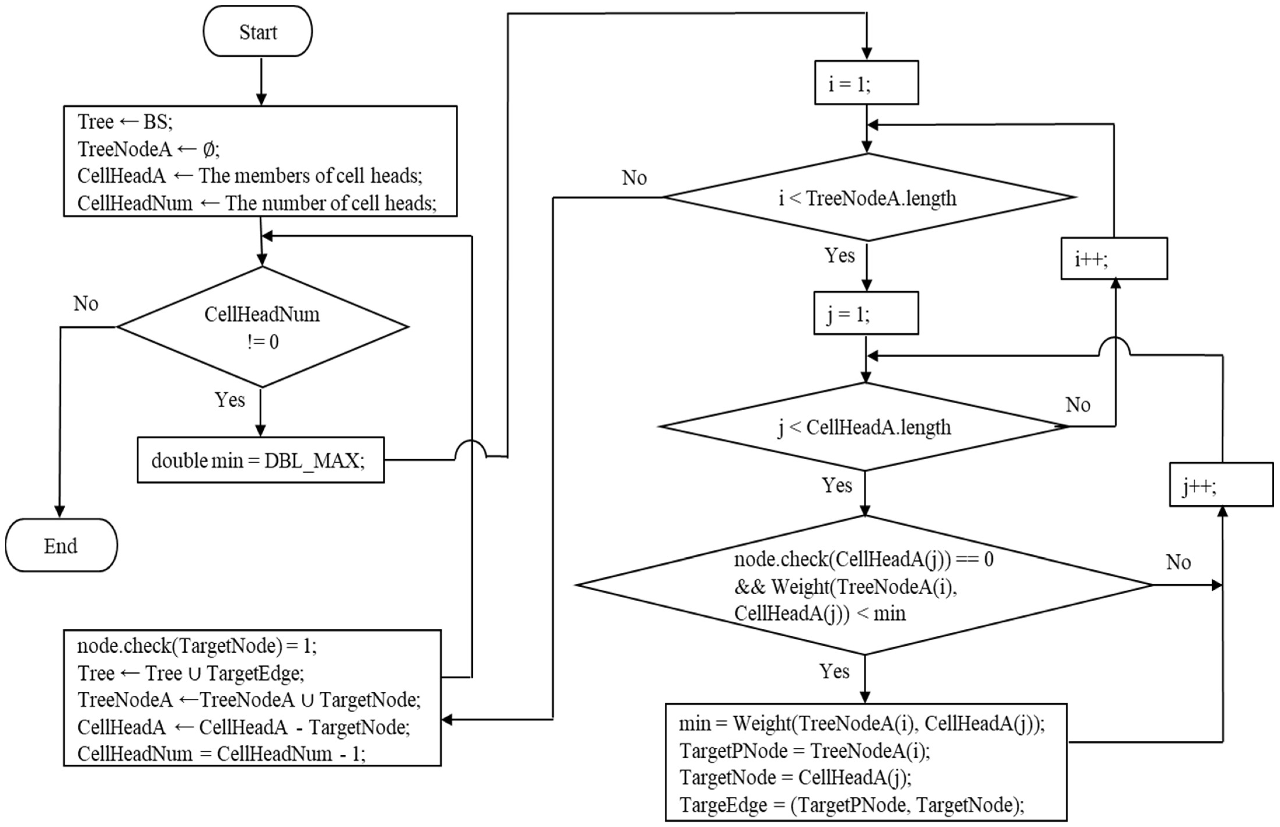
The proposed GB-PEDAP mainly uses the tree construction algorithm to continuously select cell heads until all cell heads have been added to the tree. The GB-PEDAP tree construction algorithm is shown in Algorithm 1. The flowchart of the GB-PEDAP tree construction algorithm is shown in Figure 2.

Algorithm 1: GB-PEDAP Tree Construction Algorithm.

Notations: Tree: The tree path for data aggregation CellHeadNum: The number of cell heads not added to the tree TreeNodeA: The tree node array CellHeadA: The cell head array TreeNode(i): The i-th element of TreeNodeA CellHead(j): The j-th element of CellHeadA TargetPNode: Parent node of the target node TargetNode: Target node TargetEdge: Target edge (TargetPNode, TargetNode) Weight(p, q): The weight value of the edge between node p and node q min: the minimum weight node.check(r): Determine whether node r has been added to the tree Procedure: Tree ← BS; //initialize Tree TreeNodeA ← $\varnothing$; //initialize TreeNodeA CellHeadA ← The members of cell heads not in the tree; //initialize CellHead while (CellHeadNum != 0) //do while-block until CellHeadNum is equal to 0 {   double min = DBL_MAX; // initialize min to the maximum value of the double type   for (i = 1; i < TreeNodeA.length; i++) // do for-block for each member of TreeNodeA   {     for (j = 1; j < CellHeadA.length; j++) // do for-block for each member of CellHeadA     {       if (node.check(CellHeadA(j)) == 0 &&           Weight(TreeNodeA(i), CellHeadA(j)) < min)       // if the j-th node does not in the tree and the weight of the current edge < min       {           min = Weight(TreeNodeA(i), CellHeadA(j)); // update the value of min           TargetPNode = TreeNodeA(i); // assign TargetPNode           TargetNode = CellHeadA(j); // assign TargetNode           TargeEdge = (TargetPNode, TargetNode); } // assign TargetEdge     }   }   node.check(TargetNode) = 1; // assign node.check(TargetNode) to 1   Tree ← Tree ∪ TargetEdge; // add the TargetEdge to Tree   TreeNodeA ← TreeNodeA ∪ TargetNode; // add TargetNode to TreeNodeA   CellHeadA ← CellHeadA – TargetNode; // remove TargetNode from CellHeadA   CellHeadNum = CellHeadNum – 1; // CellHeadNum decreased by 1 }

3.3. Data Transmission

In this study, data transmission begins after the tree structure is constructed. Each cell head collects sensing data from nodes in the same cell. After the cell head collects the data, they are transmitted along the paths of the tree structure, and finally transmitted back to the BS making a complete round of data transmission. At the beginning of each round, the selection and tree structure of the cell head is reset. In the proposed GB-PEDAP, by re-selecting the cell head mechanism to make the energy consumption of the cell head more uniform, the excessive energy consumption of some sensors can be avoided.

4. Simulation Results

We conducted the development of simulations with MATLAB software. The simulation parameters are given in

Table 1. Simulation parameters.

Parameters	Values
Network area	100 m × 100 m
Location of BS	(50, 150)
Initial energy	0.25 J/node, 0.5 J/node
Number of cells	5 × 5
Number of sensor nodes	100–400
Packet length	2000 bits

. In general, the number of cells is 5 × 5, the number of nodes is 200 with the initial energy of 0.25 J and 0.5 J. The proposed scheme will be compared with GB-PEDAP, PEDAP, GSTEB, and TBEEP for energy efficiency analysis.

4.1. Number of Rounds

We first explore the number of rounds under different percentages of node death. GB-PEDAP, TBEEP, GSTEB, and PEDAP are simulated, respectively, to observe the number of rounds executed when the rate of node death reaches 1%, 20%, 40%, 60%, 80%, and 100%. In Figure 3, the number of rounds executed by the proposed GB-PEDAP is better than that of TBEEP, GSTEB, and PEDAP. The number of rounds executed by GB-PEDAP is approximately 1.2 rounds of TBEEP, 1.3 rounds of GSTEB, and 1.5 rounds of PEDAP. After TBEEP is executed for a period of time, the selection of the head is progressively farther away from the BS, increasing the energy consumption of the cell head, and leading to a quicker cell death. The path of GSTEB is mainly decided by the distance; thus, the energy consumption of the sensor node is not considered. PEDAP does not consider the remaining energy of current sensor nodes when constructing the tree structure, leading to the rapid death of sensor nodes with low energy, thus reducing the lifetime of the network. GB-PEDAP mainly builds a grid structure in the sensing area and collects the data sensed by the sensors in the cell through the cell head. Since the transmission distance between the sensors is short, the energy consumption can be dispersed effectively.

4.2. Number of Alive Nodes

We study the number of alive nodes over several rounds. In Figure 4, when the initial energy is 0.25 J, we simulated the number of alive nodes for numerous rounds for GB-PEDAP, TBEEP, GSTEB, and PEDAP. The execution rounds of the first node death for GB-PEDAP, TBEEP, GSTEB, and PEDAP are 751, 572, 486, and 339, respectively. The execution rounds of the last node death for GB-PEDAP, TBEEP, GSTEB, and PEDAP are 1441, 1259, 1215, and 1092, respectively. Therefore, GB-PEDAP can extend the network’s lifetime effectively.

4.3. Number of Rounds When the First Node Dies

We observe the number of rounds when the first node dies in different nodes. In this simulation, the number of sensors is increased from 100 to 400, and is increased by 100 each time. In Figure 5, when GB-PEDAP is executed until the first node dies, the lifetime of GB-PEDAP is better compared to the other three schemes. Due to the construction of the grid structure of the sensing area, the cell head will be re-selected in each round so that the energy consumption can be effectively distributed. The transmission distance between nodes can also be shortened. When the number of nodes is increased, energy is saved because the cell head aggregates the data, thereby reducing the data transmitted and the number of data transmissions.

4.4. Total Consumed Energy

We observe the total energy consumption required by the WSN over various rounds. The number of sensors is 200 and the initial energy of the sensors is 0.25 J. Thus, the initial total energy is 50 J. In the process of data transmission, when the execution rounds increases, the total consumed energy of sensors also increases. Figure 6 illustrates how GB-PEDAP effectively reduces energy consumption compared to the other three schemes.

4.5. Energy Distribution of Sensing Area

In order to determine whether the proposed GB-PEDAP can disperse the energy consumption, the remaining energy distribution of the sensors is simulated when the first sensor dies. The number of sensors is 200 and the initial energy of sensors is 0.25 J. Figure 7 shows that the average remaining energy of GB-PEDAP, TBEEP and GSTEB is between 0.112 and 0.118, and that of PEDAP is between 0.1 and 0.123. The average remaining energy of GB-PEDAP is slightly better than TBEEP and GSTEB, and much better than PEDAP. The uniformity of energy distribution of GB-PEDAP is the best, and the uniformity of energy distribution of PEDA P is the worst. The proposed GB-PEDAP can effectively achieve uniform remaining energy distribution compared to TBEEP, GSTEB, and PEDAP.

4.6. Discussion

In this section, we discuss the differences between GB-PEDAP, TBEEP, GSTEB, and PEDAP, which are shown in

Table 2. The comparisons among different data aggregation protocols.

Protocol	GB-PEDAP	TBEEP	GSTEB	PEDAP
Hierarchical architecture	two layers	single layer	single layer	single layer
Data transmission structure	direct and tree	chain	tree	tree
Energy efficiency	high	medium	medium	low
Uniformity of remaining energy	very good	good	good	average

. The hierarchical architecture of GB-PEDAP is two layers, whereas those of the other protocols are single-layer architectures. The data transmission of GB-PEDAP contains direct transmission and tree-path transmission. The energy efficiency of GB-PEDAP is the best. The uniformity of remaining energy of GB-PEDAP is very good.

In TBEEP, the sensing area is divided into three sections. The sensor with the highest remaining energy in the first section is preferentially selected as the head as it is closer to the BS. The nodes in the second and third sections mainly transmit data to the head of the first section to the BS through the head. During the data transmission, if all the sensors in the first section are in the dead state, the head will continue to be selected for transmission to the second section until all nodes die. Due to the head selection mechanism of TBEEP, the energy consumption of the nodes that are closer to the BS is higher. Therefore, the remaining energy of sensors closer to the BS is lower, while the energy of nodes farther from the BS is higher. GSTEB selects the sensor with the highest remaining energy in the sensing area to be the root node. Each node finds the parent node according to the distance required to form a tree-like structure. Although the scheme has a strategy of balancing energy, it is possible that a node far from the BS could be selected as the root node. In this case, the energy of the node (acting as a root node) would be consumed quickly. Since the tree construction of PEDAP does not consider the remaining energy of the current sensors, PEDAP would make the energy distribution relatively unstable. However, the proposed GB-PEDAP mainly builds a grid structure in the sensing area, thus balancing energy consumption by using the cell head mechanism. Using Prim’s algorithm for a tree structure also helps to reduce the cost of the overall transmission path.

5. Conclusions

This paper proposes an energy aware clustering grid-based power efficient data aggregation protocol (GB-PEDAP) for WSNs. This scheme builds a grid of cells in the sensing area, selects the sensor with the highest remaining energy in each cell as the cell head, and uses Prim’s algorithm to connect the cell heads to build a tree structure. During data transmission, each cell head is responsible for data collection and data aggregation of sensor nodes in the cell. The cell head will transmit the data along the tree structure’s path, and finally transmit it to the BS. In the simulations, the number of rounds executed by GB-PEDAP is better than PEDAP, GSTEB, and TBEEP. The number of rounds executed by GB-PEDAP is approximately 1.2 rounds of TBEEP, 1.3 rounds of GSTEB, and 1.5 rounds of PEDAP. With the initial energy being 0.25 J, the execution rounds of the first node death for GB-PEDAP, TBEEP, GSTEB, and PEDAP are 751, 572, 486, and 339, respectively. The proposed GB-PEDAP can effectively balance and disperse the energy consumption of sensors, thereby prolonging the lifetime of a WSN.

References

- Akyildiz, I.F.; Su, W.; Sankarasubramaniam, Y.; Cayirci, E. Wireless sensor networks: A survey. Comput. Netw. 2002, 38, 393–422. [Google Scholar] [CrossRef]
- Shafiq, M.; Ashraf, H.; Ullah, A.; Tahira, S. Systematic literature review on energy efficient routing schemes in WSN—A survey. Mob. Netw. Appl. 2020, 25, 882–895. [Google Scholar] [CrossRef]
- Sharmal, S.; Kaur, A. Survey on wireless sensor network, Its Applications and Issues. J. Phys. Conf. Ser. 2021, 1969, 1–10. [Google Scholar]
- Coleri, S.; Cheung, S.Y.; Varaiya, P. Sensor networks for monitoring traffic. In Proceedings of the Annual Allerton Conference on Communication, Control and Computing, Monticello, IL, USA, 29 September–1 October 2004; pp. 883–892. [Google Scholar]
- Haseeb, K.; Din, I.U.; Almogren, A.; Islam, N. An energy efficient and secure IoT-based WSN framework: An Application to Smart Agriculture. Sensors 2020, 20, 2081. [Google Scholar] [CrossRef] [PubMed]
- Majid, M.; Habib, S.; Javed, A.R.; Rizwan, M.; Srivastava, G.; Gadekallu, T.R.; Lin, C.W. Applications of wireless sensor networks and internet of things frameworks in the industry revolution 4.0: A systematic literature review. Sensors 2022, 22, 2087. [Google Scholar] [CrossRef] [PubMed]
- Jin, C.; Valois, F. Data aggregation in wireless sensor networks: Compressing or forecasting. In Proceedings of the IEEE Wireless Communications and Networking Conference, Istanbul, Turkey, 6–9 April 2014; pp. 1–6. [Google Scholar]
- Fasolo, E.; Rossi, M.; Widmer, J.; Zorzi, M. In-network aggregation techniques for wireless sensor networks: A survey. In Proceedings of the IEEE Wireless Communications and Networking Conference, Washington, DC, USA, 1–15 March 2007; Volume 14, pp. 1–18. [Google Scholar]
- Zeng, M.; Huang, X.; Zheng, B.; Fan, X. A heterogeneous energy wireless sensor network clustering protocol. Wirel. Commun. Mob. Comput. 2019, 2019, 1–11. [Google Scholar] [CrossRef]
- Faheem, M.; Fizza, G.; Ashraf, M.W.; Butt, R.A.; Ngadi, M.A.; Gungor, V.C. Big Data acquired by Internet of Things-enabled industrial multichannel wireless sensors networks for active monitoring and control in the smart grid Industry 4.0. Data Brief 2021, 35, 1–12. [Google Scholar] [CrossRef] [PubMed]
- Faheem, M.; Butt, R.A.; Raza, B.; Alquhayz, H.; Ashraf, M.W.; Raza, S.; Ngadi, M.A.B. FFRP: Dynamic firefly mating optimization inspired energy efficient routing protocol for internet of underwater wireless sensor networks. IEEE Access 2020, 8, 39587–39604. [Google Scholar] [CrossRef]
- Amutha, J.; Sharma, S.; Sharma, S.K. Strategies based on various aspects of clustering in wireless sensor networks using classical, optimization and machine learning techniques: Review, taxonomy, research findings, challenges and future directions. Comput. Sci. Rev. 2021, 40, 1–43. [Google Scholar] [CrossRef]
- Abbi, N.; Sharma, S. Comparative review of evaluating and depleting energy hole problem in wireless sensor network. In Proceedings of the International Conference on Green Engineering and Technologies, Coimbatore, India, 19 November 2016; pp. 1–5. [Google Scholar]
- Asif, M.; Khan, S.; Ahmad, R.; Sohail, M.; Singh, D. Quality of service of routing protocols in wireless sensor networks: A Review. IEEE Access 2017, 5, 1846–1871. [Google Scholar] [CrossRef]
- Shen, J.; Wang, A.; Wang, C.; Hung, P.C.K.; Lai, C.-F. An efficient centroid-based routing protocol for energy management in WSN-assisted IoT. IEEE Access 2017, 5, 18469–18479. [Google Scholar] [CrossRef]
- Lindsey, S.; Raghavendra, C.S. PEGASIS: Power-efficient gathering in sensor information system. In Proceedings of the IEEE Aerospace Conference, Big Sky, MT, USA, 9–16 March 2002; Volume 3, pp. 1125–1130. [Google Scholar]
- Ye, F.; Haiyun, L.; Jerry, C.; Songwu, L.; Zhang, L. A two-tier data dissemination model for large-scale wireless sensor networks. In Proceedings of the ACM International Conference on Mobile Computing and Networking, Atlanta, GR, USA, 23–28 September 2002; pp. 148–159. [Google Scholar]
- Chen, T.-S.; Chang, Y.-S.; Tsai, H.-W.; Chu, C.-P. Data aggregation for range query in wireless sensor networks. In Proceedings of the IEEE Wireless Communications and Networking Conference, Hong Kong, China, 11–15 March 2007; pp. 1–6. [Google Scholar]
- Bandral, M.S.; Jain, S. Energy efficient protocol for wireless sensor network. In Proceedings of the Recent Advances and Innovations in Engineering, Jaipur, India, 9–11 May 2014; pp. 477–482. [Google Scholar]
- Han, Z.; Wu, J.; Zhang, J.; Liu, L.; Tian, K. A general self-organized tree-based energy-balance routing protocol for wireless sensor networks. IEEE Trans. Nucl. Sci. 2014, 61, 732–740. [Google Scholar] [CrossRef]
- Tan, H.-O.; Lu, I.-K. Power efficient data gathering and aggregation in wireless sensor networks. ACM SIGMOD Rec. 2003, 32, 66–71. [Google Scholar] [CrossRef]
- Kaplan, E.D. Understanding GPS: Principles and Applications; Artech Hourse: Boston, MA, USA, 1996; pp. 20–25. [Google Scholar]
- Heinzelman, W.R.; Chandrakasan, A.; Balakrishnan, H. Energy-efficient communication protocol for wireless microsensor networks. In Proceedings of the Annual Hawaii International Conference on System Sciences, Maui, HI, USA, 7 January 2000; pp. 3005–3014. [Google Scholar]