Abstract
This research aimed to investigate the relationship and the correlation between abdomen fat accumulation and the level of diffused fat in the human liver using computerized methods. Computed tomography data sets of 125 subjects were employed in this study. This investigation was implemented through three phases. For each subject, the quantity of abdomen fat was measured, and then the liver was segmented and analyzed to evaluate the fat content. Finally, the collected results were utilized to evaluate the correlation. In addition, the liver intensities were measured to evaluate the level of the diffused fat in the liver. Experimental results show that there was a medium negative correlation between the visceral fat to the abdomen size ratio and the mean of the liver intensity values. The same correlation was found between the mean of the liver intensity values and the total abdomen fat to the abdomen size ratio. The ratios mentioned above were used to obtain relative measurements for the size contribution of fat (for each type) to the whole size of the abdominal area, due to the wide variety of sizes of subjects used in this research. This study supports the research community with objective measurements that reveal a direct proportional relationship between obesity and the level of diffused fat in the liver. The findings of this research provide evidence of a detrimental health effect of abdominal obesity (especially visceral fat) on liver fat content, which is associated with an increased risk of serious health problems, such as diabetes, high blood pressure, kidney disease, and developing heart problems. The research helps to identify a cause for fat accumulation in the liver, which can help in the process of preventing and treating fatty liver disease.
1. Introduction
The issue of obesity and overweight has become a global health concern. It is proven that overweight and obesity have an adverse effect on health, leading to reduced life expectancy and increased health problems. Furthermore, overweight and obesity are major risk factors for several chronic diseases, including diabetes, cardiovascular diseases, cancer, chronic kidney failure, and liver problems. Non-alcoholic fatty liver disease (NAFLD) is a term used to describe the accumulation of fat in the liver of people who drink little or do not drink alcohol at all. The fat that accumulates in the liver can cause inflammation and scarring in the liver, which can progress to liver failure. Experts believe that fat accumulation in the body (especially in the abdomen region) is correlated with non-alcoholic fatty liver diseases, since these diseases are related to insulin resistance, which is a condition closely associated with obesity [1,2,3,4,5]. Statistical analyses and studies that link liver diseases to obesity are usually based on measuring obesity in patients who have been diagnosed with liver disease. Measuring obesity using one of the traditional procedures, such as calculating the body mass index (BMI) or measuring the thickness of the subcutaneous abdomen fat using a clipper, does not provide a quantitative measurement of body fat. Yet, no study has derived an accurate objective measurement for the correlation between the actual quantity of abdomen fat and the level of diffused fat in the liver.
Fat infiltration in the liver can occur in many different patterns. Diffuse fatty infiltration involving the entire liver is the most common pattern. According to Hamer et al. [6], the attenuation of the normal liver is slightly greater than the spleen in non-contrast-enhanced computed tomography (CT) images. Based on this observation, diffused fatty liver can be recognized if the attenuation of the liver is at least 10 HU less than that of the spleen, or if the liver attenuation is less than 40 HU. Other CT criteria have been advocated by Ricci et al. [7]. They measured the liver to spleen attenuation ratio and clarified a ratio of less than 1 as indicative of fatty liver. They quantified the liver fat using non-contrast-enhanced CT images. In contrast-enhanced CT images, comparing the attenuation values of the liver and spleen is not as reliable for fatty liver diagnosis, because the differences between the liver and spleen attenuations depend on the timing and the technique used, and also because there is an overlap between normal and abnormal liver attenuation value ranges [8,9]. Ricci et al. [7] stated that fatty liver can be diagnosed using contrast-enhanced CT images if the attenuation absolute value is less than 40 HU. CT scanning provides a useful non-invasive method for detecting and following patients with fatty liver, particularly when the liver biopsy is contraindicated [10]. According to Kodama et al. [11], measurement of attenuation of the liver using non-contrast-enhanced CT scans is best for the prediction of pathologic fat content in the human liver.
Physicians and experts believe that overweight people are more likely to develop a fatty liver. Nugent and Younossi [12] presented an interesting study, where 24 patients diagnosed with non-alcoholic fatty liver were subjected to 3 months of a low-calorie diet. For each patient, CT examinations were performed before and after the 3 months of a low-calorie diet. Results show that the attenuation values on CT scans after 3 months of the diet were increased for each patient. This observation indicates that the level of diffused fat in the liver had decreased. Jakobsen et al. [5] evaluated epidemiologic evidence for an association between abdominal fat and liver fat content. They state that some studies using waist circumference to estimate abdominal fat mass suggested a direct association between abdominal fat and liver fat content. Other studies using imaging methods suggested a direct association between intraabdominal fat and liver fat content, but not between subcutaneous abdominal fat and liver fat content. In conclusion, clinical and epidemiologic studies of abdominal fat and liver fat content suggest a direct association between abdominal fat and liver fat content, which is probably accounted for by visceral fat. Many researchers have attempted to study the relationship between obesity and fatty liver diseases to provide more clarification about the concerned correlation [13,14,15]. By reviewing their obtained results (regardless of the size and nature of the employed data and the method used), it can be noticed that there is some similarity. Table 1 shows the method used, the size of the data set, and the results of each study.

Table 1.
Obesity and fatty liver correlation study comparison.
Fernando et al. [16] investigated the correlation between obesity and NAFLD using the weight, BMI, and excess weight of a data set of subjects as measurements for obesity. They stated that NAFLD was closely correlated with type 2 diabetes (T2DM), insulin resistance, and dyslipidemia (LDL cholesterol), but was not with the size of the patient (weight, BMI, and excess weight). Using the size of the patient as a measurement of the abdominal fat has a few limitations. Size is an indirect and imperfect measurement of obesity, and it does not distinguish between total body fat and lean body mass; it is not an accurate predictor of the body fat in the elderly, and at the same BMI, it has been found that body fat depends on the sex and race of the subject [17]. Therefore, using weight, BMI, or excess weight as a measurement of the accumulation of fat in the abdomen region of the human body is not an accurate measure. In contrast, CT and magnetic resonance imaging (MRI) are accurate techniques, and they allow for the measurement of specific body fat compartments, such as abdominal fat, visceral fat, and subcutaneous fat [17].
Generally, experts and physicians believe that the quantity of abdomen fat accumulation and the diffusion of fat in the liver are proportional (more accumulation of abdomen fat leads to a higher degree of diffusion of fatty liver disease). There is a hypothesis that visceral fat produces free fatty acids, which exposes the liver to fat accumulation [18]. This research aimed to evaluate this hypothesis technically and statistically to find evidence for an association between abdominal fat and liver fat content. This current research also supports the research community by providing objective measurements to approve this direct proportional relationship, derived from an investigation of the relationship mentioned above. Two computerized/adaptive methods for abdomen fat segmentation and liver segmentation were proposed. No training data were used to estimate any global parameters or to create models. A hybrid segmentation method was proposed to segment the non-contrast-enhanced CT slices into fat and non-fat tissues. Then, the segmented fat tissues in each CT slice were separated into subcutaneous fat (SF) and visceral fat (VF) by detecting the abdomen wall boundary. Finally, the segmented fat tissues were used to quantify the abdomen fat accumulation for each subject. The whole liver segmentation procedure was based on processing the CT slices one by one. Many image processing techniques and anatomic information were employed together to segment the liver in each CT slice. The slices of the segmented liver in the CT were gathered to form 3D binary liver data. This 3D binary image was refined to produce the final segmented liver for a subject. Then, the diffused fat in the segmented liver was evaluated by measuring the liver attenuation (measured in Hounsfield units (HU)) for the segmented liver for each subject. The lower the average values of the liver intensities, the lower the tissue density, and hence, the greater the fat content. The obtained measurements of the abdomen fat and the liver attenuation for the employed data set were used to draw a general figure for the correlation between these two effective factors of human health.
The main contribution of this research is the use of the indexes of abdomen fat and whole liver HU mean values to highlight the relationship between obesity and fatty liver disease. To achieve this goal, methods with high stability, consistency, and accuracy were designed. In addition to the main contribution, other contributions derive from this research. In the fat segmentation method, a modification was made to the FCM clustering technique to increase the ability of the method to detect the abdomen wall. The combination of FCM and Otsu thresholding, on the other hand, helped to achieve a great degree of stability and consistency for the fat segmentation method. Another contribution was made by introducing an approach toward refining the segmented liver using the distance transformation technique. The proposed liver segmentation method successfully limited the effects of problems such as the high inter- and intra-CT gray level, shape, and size of liver variability on the results of liver segmentation.
2. Liver Segmentation and Abdominal Fat Segmentation/Classification Methods
Methods presented in the literature to obtain liver segmentation were reviewed in detail by Mharib et al. [19] (Mharib is the formal last name of Ahmed Alkinani, who is one of the authors of this research). In this review, liver segmentation methods are divided into two categories: semi- and fully automatic methods. For each category, several methods, approaches, related issues, and problems were defined and discussed. Mharib at. al. [19] found that gray-level-based techniques obtain the most promising results among the reviewed methods, but they are not robust to database variations. Gray level estimation does not consider the high variability of CT intensity values. Therefore, the performance could decrease significantly when larger and more complex data sets are used. Additionally, most methods require manual intervention and for some critical parameters to be experimentally estimated. It was also found that learning techniques are strongly dependent on the training set. Model-based techniques and probabilistic atlases suffer from the same difficulty: they need a lot of data to be properly collected and manually segmented to produce the model. In addition, processing non-standard liver shapes increase the chances for the algorithms to fail.
The fat tissue normal CT attenuation is defined based on Hounsfield units (Hu) as the interval within (−190 < Hu < −30) [19,20,21]; the average of the fat tissue attenuation varies across subjects, and it depends on the CT scanner used [20]. Tohru et al. [20] proposed a method to estimate the abdominal fat distribution using a threshold within the mean ± two standard deviations. This method did not consider the spatial relationship of the pixels. Their method included some user interaction to calculate the mean and the standard deviation to separate the SF from the VF. Romero et al. [21] included a semi-automatic method to separate the two types of fat from each other. Two binary masks were created, one for the skin of the subject and the other for the abdomen wall. Pixels between these two masks were classified as SF, and pixels inside the mask of the abdomen wall were classified as VF. However, the classification of the fat tissues was based on a fixed interval of intensities, and user interaction is required to remove any artifact that may appear in the CT image.
The analysis of histograms was introduced by Zhou et al. [22] in their human structure recognition system, where the CT images were divided into four parts (air, fat, organs and muscles, and bones) based on the distribution of these tissue intensities. A dynamic process was applied to estimate the gray-level threshold values to implement the segmentation operation. To separate the SF from the VF, the distances between the skin pixels and muscles/organs were calculated using the Euclidean distance transformation algorithm. The measured distances were used to extract the SF from the fat binary image. The fat regions, except the extracted SF, were considered as the VF. Pednekar et al. [23] presented an automatic abdomen fat tissue segmentation method that combined intensity and texture information; this combination was then used as an input to the FCM clustering technique to implement the segmentation task. They found that the combination of intensity and spot–spot texture feature (derived from Laws’ features) provided the highest discrimination between fat and non-fat tissues. Statistics of fat tissues were calculated by automatic selection of several seed points using an active shape model, and a template was constructed to separate the SF from the VF tissues. Considering the texture as a feature in the fat segmentation methods requires a process to find the best texture features that describe the fat tissues. Therefore, training data must be collected and labeled manually, and then the combination of the most discriminating features must be selected. The results of the feature selection operation depend on the collected data and the technique used to find the combination of the most discriminating features. This explains the contradictions in the results of feature selection operations, which have been included in the processing of CT images in a lot of research studies.
3. Materials and Methods
This prospective study included a total of 125 patients. The data set of 35 subjects (20 male subjects, 36 to 62 years old, mean age 49 years; 15 female subjects, 37 to 72 years old, mean age 51 years) was acquired using SIEMENS scanner at Country Heights Health Tourism Sdn. Bhd. Scanning was performed at 130 kV and 200 mA. The resolutions of the slices were 512 × 512 pixels, and the slice thickness was 2.5 mm in all subjects. The data set of the remaining subjects (57 male subjects, 24 to 72 years old, mean age 46 years; 33 female subjects, 26 to 70 years old, mean age 50 years) was acquired using a TOSHIBA scanner at the hospital of Serdang. Scanning was performed at 120 kV and 200 mA. The resolutions of the slices were 512 × 512 pixels, and the slice thickness was 2 mm or 3 mm. Both health centers are in the state of Selangor, Malaysia. The data set used is not publicly available due to the rights of Country Heights Health Tourism Sdn. Bhd and the hospital of Serdang located in Malaysia. Figure 1 shows some CT image samples from the employed data set.
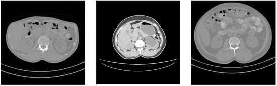
Figure 1.
CT image samples.
For each subject in this investigation, the data set was processed through three main stages. In the first stage, an automated method of segmenting and classifying abdomen fat was implemented using CT images. The segmented fat tissues in the abdominal region of the subject were classified as SF and VF. In the second stage, an automated method of liver segmentation method using CT images was implemented, and the segmented liver was employed to evaluate how fatty the liver was. In the last stage, the results obtained from stage one and stage two were analyzed to evaluate the correlation between the level of diffused fat in the liver and obesity. The employed images in this research are gray-scale non-contrast-enhanced CT images stored in DICOM format. Figure 2 shows a block diagram of the methodology.
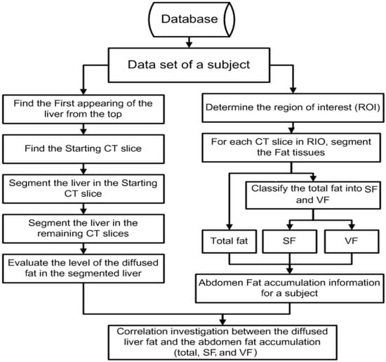
Figure 2.
Block diagram of the methodology.
A fully automatic liver segmentation method using non-contrast-enhanced CT images was used in this research. In this method, the liver is segmented into slices one by one. Gray level, Gaussian gradients, region growing algorithm, distance transformation, canny edge detector, and anatomic information play the main roles in the liver segmentation method. The details of the liver segmentation method used in this research have been published by one of the authors of this research [24]. The first slice (Iss) was selected automatically from the data set of a subject where the liver covers a wide area. The segmented liver in Iss is used as a reference for the adjacent slices. The same employed techniques to segment the liver in the starting slice are employed to segment the liver in all other CT slices of the subject. Whenever the liver in a new slice is segmented, it will be used as a reference for the next slice. The procedure will keep going in this manner until it reaches the top of the liver and the liver’s bottom lobe. Figure 3 shows the structure of the proposed method.
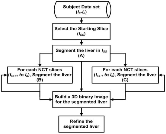
Figure 3.
The structure of the proposed liver segmentation method.
The procedure of segmenting the liver in the starting slice is presented in the following steps:
- Finding the slice where the liver starts to appear.
- Finding the liver seed region.
- Calculating the liver parameters.
- Selecting the starting CT Slice (Iss).
- Segmenting the liver in Iss.
4. Finding the Slice Where the Liver Starts to Appear
In the beginning, CT slices for a subject were searched from the top to the bottom for the slice that contains the first appearance of the liver. Every two sequenced CT slices separated by two slices were binarized using the Otsu thresholding technique, and whenever the liver started to appear, the number of white pixels on the left side of the image increased extensively. The summation for the white pixels on the left side for each slice was calculated. These two values were subtracted from each other, and whenever a result of a positive value greater than a specific threshold value was found, the search process was ended, and the CT slice at that point was considered as the CT slice where the liver starts to appear. This slice will henceforth be referred to as the liver top image.
5. Finding the Liver Seed Region
To segment the liver in Iss, a pure liver region is needed to calculate some important parameters. In the liver top image, the liver was barely noticeable. In the slices that followed, the cross-section area of the liver started growing slice by slice. By considering the liver top image as a reference and selecting the 10th CT slice (the counting started from the liver top image), some similarity in the left sides of both images was observed, except for the liver region in the 10th CT slice, where a region of the liver was noticed. To segment this region, both images were binarized using the Otsu thresholding technique. By subtracting the liver top image from the 10th slice image, and only considering the left side of the resulting image, a binary image of the liver region and some small isolated regions were produced. This image was filtered using morphological filtering that only kept the region with the maximum number of foreground pixels.
6. Calculating the Liver Parameters
Once the liver seed region was detected, another four slices were selected. Each two sequenced CT slices of these five slices were separated by one slice. Only pixels that share same the coordinates with the liver seed regions were used. The mean and the standard deviation for the gray level intensities of these pixels in the five slices were calculated. A gradient transformation using the first-order derivative of Gaussian was also employed. The gradient transformation was determined using a 2D Gaussian kernel, where the standard deviation of the kernel was defined as a positive variable. For each CT image of the previously mentioned five CT images, three gradient images were produced: the horizontal, the vertical, and the diagonal gradient images. The same procedure that was used to separate the liver pixels was applied to the gradient images, and a set of six parameters were produced: the liver’s mean horizontal, vertical, and diagonal gradients, and the liver’s standard deviation horizontal, vertical, and diagonal gradient. At the end of this stage, eight different parameters were produced to detect the initial liver region in the starting slice.
7. Selecting the Starting CT Slice
By starting counting from the liver top slice, the 25th, 30th, and 35th slices were selected as candidates to be the starting slice. Based on the distance between the CT slices and the anatomic information of the liver, a suitable candidate for the starting CT slice could be found between the 25th and 35th CT slice, where the liver must cover a large area of the CT slice, and should be presented as one connected region. The liver in all of these slices was segmented, and the slice with one region of the liver with the maximum cross area was selected as the starting slice.
8. Segmenting the Liver in Iss
The process of segmenting the liver in the Iss can be summarized in the following steps:
Step 1: Threshold the Is image using the liver’s intensity parameters and remove the skin, abdomen wall, spleen, and any artifact that may appear in the binary image.
Step 2: Find the liver seed region using gradient transformation, gradient parameters, and the binary image from Step 1.
Step 3: Apply the region growing algorithm using the liver seed region and the diagonal gradient image to segment the liver in the CT slice initially.
Step 4: Extend the initial segmented liver until it meets with the actual boundary of the liver.
Segmenting the liver starts with thresholding Iss image using the mean (Mi) and the standard deviation (Si) parameters, as shown in the following formulas:
In both binary images Isab1 and Isab2, the liver was segmented, in addition to the other organs and tissues that shared the same gray level intensities with the liver. The component a2 was assigned a specific value to ensure that foreground pixels in Issb2 are connected, which will help in the process of removing the skin, the abdomen wall, and the spleen correctly. The component a1 was assigned to a value less than a2. Thresholding Iss images using Equation (1) helped to reduce the error of segmenting the attached organs and considering them as a part of the liver.
The skin was removed from Issb2 and the boundary of the abdomen wall was detected and dilated morphologically using a specified structural element. After that, simple logic and operation between the skin-removed version of the Issb2 binary image, and the inverse of the dilated abdomen wall boundary binary image, were implemented. After that, a box boundary around the resulting region was created, and the right bottom quarter was removed. This operation helped to remove the spleen and to reduce the processing area since the liver does not exist or appear in that part. Finally, element-wise logic and operation between Issb1 and processed Issb2 was implemented to remove the skin, the abdomen wall, and the spleen tissues from Issb1.
The liver initial region in the Iss image was segmented next. This region was used as the seed for the region growing algorithm. Finding the liver seed region started with applying the Gaussian gradient transformation on Iss to produce three gradient images: horizontal, vertical, and diagonal. The region with the maximum number of foreground pixels in Issb1 was selected and multiplied by each one of the gradient images (corresponding elements were multiplied and return the product in the corresponding elements of the output). The resulting images (Iss1, Iss2, and Iss3) were thresholded after that using the gradient parameters, as shown in the following equation.
Element-wise logic and operation were applied on the three binary images that resulted from the thresholded operation, followed by a morphological filtering process to produce the liver seed region. The image that contains the liver seed region will be referred to as Ls binary image. Figure 4 shows two samples of the starting CT slices for two subjects and their segmented liver seed results. The third column in Figure 4 shows the boundary of the liver seed region inside Iss.
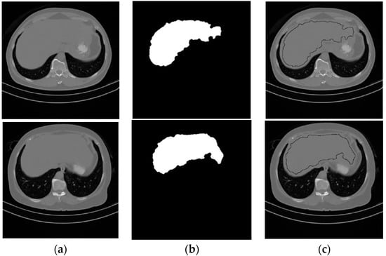
Figure 4.
Samples from the liver seed segmentation results. (a) Original, (b) seed segmented liver, (c) boundary of the seed segmented liver.
Liver seed region pixels in Ls were considered as correct segmented liver, and the boundary of the liver seed region with the diagonal gradient image (elementary-wise multiplied by Issb1) was employed as an input to the region growing algorithm. The region growing algorithm was based on creating a 2D matrix (RGM). This matrix consisted of three columns and an unspecified number of rows. The horizontal coordinates, vertical coordinates, and diagonal gradient values for each boundary pixel were stored in a row in RGM. In the beginning, each pixel in Ls was assigned one of three different values: 2 as a liver pixel, 1 as an added pixel to RGM, and 0 as an un-added pixel to RGM. Pixels of the liver in the diagonal gradient image is extracted using the liver seed region, and the mean (Mg) and the standard deviation (Sg) values were calculated. The implementation of the region growing process is presented in Algorithm 1.
| Algorithm 1. |
| Mp = 0; |
| While (Mp < Thmp) |
| [Mp index] = mini ([3rd column of (RGM)]-Mg|) |
| [X Y] = RGM(index) |
| Ls(X, Y) = 2 |
| For i = −1 to i = 1 |
| For j = −1 to j = 1 |
| If Ls(X + i, Y + j) = 0 & |Dg(X + i, Y + j)-Mg| < Sg |
| Add Dg(X + i, Y + j) to RGM |
| Ls(X + i, Y + j) ←1 |
| end |
| end |
| end |
| Remove RGM (index) |
| End |
| Liver_image ← [Ls = 2] |
Thmp was specified a threshold value greater than zero, and Mp was a value initialized to zero at the beginning of the implementation and was updated later. The mini function returns the minimum absolute value of subtracting the diagonal gradient values stored in the 3rd column of RGM from the Mg value and assigns it to Mp. The mini function returns the index of the minimum absolute value as well. The row in RGM pointed by the index contained the location of a pixel, which will be considered a liver pixel. After that, the eight neighbor pixels of the current liver segmented pixel were tested to check whether each one should be added to the RGM or not. Then, the row that contained the current liver pixel segmented information was removed from RGM. The iteration process was continued in this manner until all the diagonal gradient values stored in RGM were greater than Thmp. Finally, the segmented liver in the Iss using the region growing algorithm was processed using morphological close operation.
In some cases, the result of segmenting the liver in Iss from the previous step did not reach a satisfactory level. To improve the segmentation result, a new method to extend the segmented liver region until it reaches the actual boundary of the liver was proposed. Each pixel in the boundary of the segmented liver was dilated using a disk structural element. The size of the structural element for each dilated pixel was adaptive and depended on the distance between that pixel and the nearest edge pixel in the actual liver within a specific condition. The method is presented as follows:
Step 1: Apply canny edge detection on Iss. The resulting binary image will be referred to as CE.
Step 2: Find the boundary of the initial segmented liver.
Step 3: Compute the Euclidean distance (ED) using CE. Each pixel is presented by the distance between that pixel and the nearest non-zero pixel of CE and the index of the nearest non-zero pixel of CE.
Step 4: Locate the coordinates of the segmented liver boundary pixels in EDT using the binary image from Step 2.
Step 5: Liver boundary pixels that are indexed to the same nearest non-zero pixel of CE are grouped and dilated using a disk structural element. The size of the structural element is equal to the minim distance in the group.
Step 6: The resulting image is added to the initial segmented liver and morphologically filtered and smoothed.
For a better understanding of the proposed method, the following illustration is presented. In Figure 5a, the inner oblong can be considered as the boundary of the initial segmented liver, and the outside edge map can be considered as the results of the canny edge detection operation. In many cases where attached organs are present, the canny edge usually failed to find the edge between the liver and the attached organs. Here, the edge map demonstrates a case where an oblong object is attached to a circular object, and they both share the same gray scales.
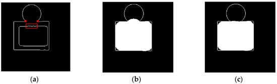
Figure 5.
Liver segmentation enhancement method demonstration. (a) Original case, (b) result of the conventional dilation, (c) result of the proposed dilation.
Figure 6 shows the result of segmenting the liver in Iss for two subjects. To the left, the initial segmentation results are shown, and to the right, the results of applying the proposed enhancement method are shown.
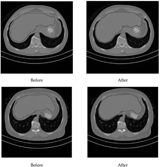
Figure 6.
Final liver segmentation in the starting slices.
At this stage, the liver was completely segmented in Iss. Next, the liver in the previous and subsequent CT slices in the data set of a subject was segmented. The same process explained for Iss was repeated for each CT slice with some modifications. The liver segmentation process for each CT slice can be summarized as follows:
Step 1: The previous segmented liver is eroded using an adaptive structural element. The size of the structural element depends on the size of the segmented liver.
Step 2: The projection of the eroded region on the current CT slice is used to find new parameters. The current CT slice is thresholded using the new parameters. The eroded region will also be used as the seed region on the region growing algorithm.
Step 3: Skin, abdomen wall muscles, and the right bottom quarter of the current CT slice is removed, and the region growing algorithm is applied to the current CT slice as in Iss.
Step 4: Elementary logic and operation between the resulting binary image from applying the region growing algorithm and the segmented liver in the previous CT slice are applied.
Step 5: Finally, the liver extension method is applied to the resulting image
The operation in Step 4 is very important in case an attached organ started to appear, and the region growing algorithm did not stop at the actual boundary of the liver. In these cases, the growth of the liver region passed the liver to the attached organ. Because the size of the liver region in subsequent CT slices was almost the same, applying the elementary logic and operation between the segmented liver and the region growing result image eliminated the attached region from the segmented liver. Applying the liver extension method on the current processed CT slice after this helped to improve the final segmented liver in the current slice. Segmenting the liver slice by slice was continued in this way until the size of the segmented liver reached a specified small size.
The human liver has two large sections, called the right and the left lobes. These two lobes usually appeared in some CT slices as two separate regions. In such cases, the proposed method handled each region separately, and the final results for both regions were combined. The first point in the modification list states that the segmented liver from the previous CT slice was eroded. If the liver in this CT slice is presented in two regions, there is a strong chance that the liver region with the smaller size was removed because of the erosion operation. Therefore, each region was eroded separately using a structural element where its size depended on the size of the region. In the proposed method, Iss subsequent CT slices were tested individually (one by one) to check whether the liver in the previous CT slice was segmented as two regions or one region.
The automatic abdomen fat segmentation method used in this study is a robust method that is employed to detect and classify the abdominal fat in non-contrast-enhanced CT images. In this method, a modified fuzzy c-means (FCM) [25,26] clustering technique and the Otsu thresholding technique [27] were used to segment fat tissues. A non-fat binary image was used to detect and trace the boundary of the abdominal wall. This boundary was used to separate SF from VF. The process of detecting this boundary started with finding the boundaries of regions in a non-fat binary image (after removing the bed and any artificial elements that may appear). The non-fat binary image was scanned top to bottom, bottom to top, left to right, and right to left. During the scanning operation, whenever a foreground pixel was detected, the scanning in that line was terminated, and the detected pixel was considered as an abdomen wall boundary pixel. Every single pixel in this boundary image must be connected to two other pixels; if a pixel was detected with one or no connected pixels, it was connected to the nearest one or two boundary pixels.
Figure 7 shows some examples of the obtained results of the constructed abdominal wall using the proposed method.
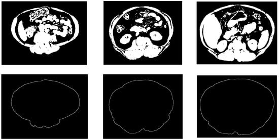
Figure 7.
Samples from the abdomen wall boundary detection results. The top row is the non-fat binary images, the bottom row is the abdomen wall boundary images.
A special condition was added to the FCM clustering technique to improve the ability of the system to detect thin parts of the abdominal wall. Additionally, the added condition helped to increase the connectivity among the abdominal wall regions, and reduced the chances of eliminating parts of the abdominal wall during the detection process for the abdomen wall boundary. This special condition also increased the system’s ability to detect fascia tissues. Therefore, a set of morphological filters were employed to eliminate these tissues for better detection of the abdominal wall boundary. Non-contrast-enhanced CT images provide good contrast between fat and non-fat tissues, which makes the total abdomen fat segmentation operation using CT images a relatively easy operation.
The classification of abdominal fat tissues deserves special attention. In the proposed method, we studied all the issues relating to the classification operation and considered them during the design stages. Figure 8 shows the structure of the proposed abdomen fat segmentation method.
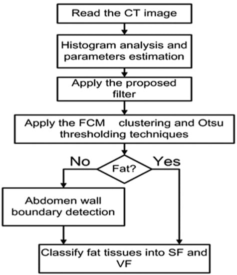
Figure 8.
Structure of the abdomen fat segmentation method.
The fat classification method started by segmenting the SF from the fat binary image by applying element-wise logic and operation between the fat binary image and the inverse of the filled abdomen wall boundary image. Subtracting the SF binary image from the fat binary image produced a binary image where foreground pixels represented the VF. Figure 9 shows the steps of the classification process illustrated by an example.
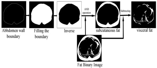
Figure 9.
SF and VF classification operation.
9. Results and Discussion
Two expert radiologists were asked to evaluate the performance of the proposed fat segmentation and classification method and the liver segmenting method. They reported that in one subject, the liver was segmented with a major error. The reason for this observation is that the proposed method failed to segment an abnormal lesion in the left lobe for that subject. Regardless of this case, the livers in all the other subjects were ranked as well segmented with minor error. According to the ability of the method to distinguish liver tissues from non-liver tissues, the radiologists reported that the method shows good capability to implement the task. However, the radiologists noticed that in some rare cases, small parts of the gallbladder and bowel were segmented as a liver. They ranked this error as a minor error. Additionally, they reported that the total fat segmentation results in all of the employed CT images were acceptable. The separation of SF and VF was accepted in almost the entire employed image. Only 0.174% of the employed images failed to detect a correct boundary for the abdomen wall. In these cases, parts of the SV were classified as VF, and in some other cases, the VF was classified as SF.
In total, 300 CT images were employed to evaluate the proposed fat segmentation classification method objectively. These CT images were manually segmented by expert radiology. These 300 CT slices were selected from 30 subjects (10 CT images/subject). The selected CT images were chosen between the first and fifth lumbar vertebrae (L1–L5). The manually segmented CT images were compared to those produced by the proposed fat segmentation classification method. Subjectively, the proposed fat segmentation classification method was also evaluated. For each subject, the fat tissues in the entire CT images between L1 and L5 were segmented and classified by the proposed method, and the results were evaluated by two radiologists.
Experimental results show that the performances of the abdominal fat segmentation method and the liver segmentation method are very promising. The abdominal fat segmentation method shows a strong capability to handle a wide variety of abdominal wall shapes. The liver segmentation method also shows good performance. Several challenges and difficulties due to the similarity of gray level intensities of the liver and the attached organs have been overcome in the proposed liver segmentation method.
The average of the accuracy and the mean error rate for the total fat, SF, and VF for the used data set (300 CT images) were used to evaluate the performance of the fat segmentation and classification method. The fat-segmented and classified data collected from the two expert radiologists were used to classify the fat pixels segmented and classified by the study method. The accuracy was defined as the percentage of correctly classified pixels (fat and non-fat) with respect to the total number of pixels in the images, whereas the mean error rate was defined as the percentage of incorrectly classified pixels (fat and non-fat) with respect to the total number of pixels in the images. The average accuracies for the three types of fat (total fat, subcutaneous fat, and visceral fat) were found to be in the range of 98.52 % to 99.95%, and mean error rate is found to be in the range of 0.4% to 1.48%.
Figure 10 shows some CT sample images and the results of fat segmentation and classification. The top row images are the original DICOM images, and the bottom row presents the results of fat segmentation and classification for the top DICOM images. The red color region represents the VF tissue, and the turquoise color region represents the SF tissues.
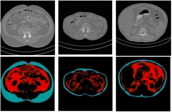
Figure 10.
Samples of the original CT images and the results of fat segmentation and classification.
The liver segmentation method was evaluated subjectively by the same two radiologists. For each subject, the radiologists were asked to evaluate the results of the segmented liver in each CT data set based on his/her observation. In addition to the subjective evaluation, the liver segmentation method was evaluated objectively by comparing the results obtained by the manual segmentation with the results obtained by the proposed method. Only three data set of three subjects were included in the objective evaluation process due to the difficulty of the manual segmentation of the liver in non-contrast-enhanced CT data and the extensive time required. The true positive rate was used to express the percentage of a true segmented liver, while the false positive rate was used to express the percentage of the non-liver tissues that were mistakenly segmented by the proposed method. Table 2 shows the obtained true positive and false positive rates for the three subjects.
Table 2.
Abdomen fat segmentation and classification method results.
Figure 11 shows side and front views for two subjects where the liver is bounded by black contours.
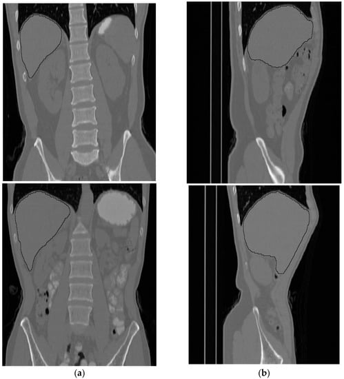
Figure 11.
Two samples of the results of the liver segmentation method. (a) Front view, (b) side view.
A general observation of the total results of applying the proposed liver segmentation method to the entire 30 subjects shows that the method successfully implements the segmentation operation. Additionally, the proposed method shows robustness in the capability to separate non-liver tissues from liver tissues.
The volumetric information for the total abdomen fat, SF, and VF does not provide realistic information about obesity due to the variation in the sizes of people. Therefore, the following ratios were used as an indication of obesity. For each subject, CT slices between the first and fifth lumbar vertebrae (L1–L5) were used. Figure 12 shows two samples that highlight the area where the CT slices were selected from. The region of interest is bounded by the two white lines.
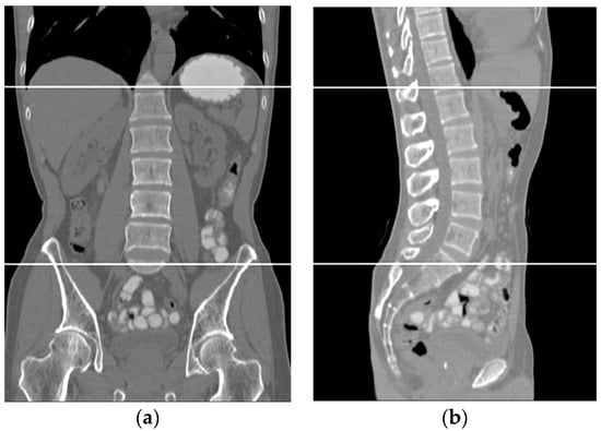
Figure 12.
Two samples show the area where the CT slices are selected from. (a) Front view, (b) side view.
The segmented and classified non-contrast CT slices for each subject were used to calculate the following ratios (total fat ratio “TFR”, subcutaneous fat ratio “SFR”, and visceral fat ratio “VFR”):
The reason for using the ratios mentioned above instead of the actual number of pixels is the subjects’ size variety. The number of fat pixels in a tall, non-obese subject might be greater than the number of fat pixels in a short, obese subject. Therefore, the ratios were used as an indication of obesity (percentage of fat in the abdominal region) for a subject.
Liver density is inversely related to liver fat, according to Ricci et al. [7]. The mean of the liver HU values for the used data set was employed as an indicator for the level of diffused fat in the liver. Figure 13 illustrates two examples of two CT images (two different subjects) where the liver is bounded by black contours using the proposed liver segmentation method. The liver in each example shows different tissue densities.
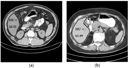
Figure 13.
Variation of liver HU values. (a) Low HU value, (b) high HU value.
To study the relationship between the accumulated abdomen fat ratios and the liver diffused fat, the correlation coefficient (R) and the p-value were used. Correlation is a statistical measurement of the relationship between two (or more) variables. Correlation coefficients range from +1 to −1. A zero correlation indicates that there is no relationship between the variables. A correlation of −1 indicates a perfect negative correlation, meaning that as one variable goes up, the other goes down. A correlation of +1 indicates a perfect positive correlation, meaning that both variables move in the same direction together. The p-value is the probability of the correlation coefficient to be in fact zero (null hypothesis). If this probability is lower than the conventional 5% (p < 0.05) the correlation coefficient is called statistically significant. The p-value in this study represents the probability that the correlation between fat ratios and Liver HU average in the used sample data occurred by chance. A p-value of 0.07 indicates that there is a chance of 7% that results from the used data occurred due to chance. A p-value of 0.02 indicates that there is only a 2% chance. Therefore, a lower p-value is a good sign that the finding of the correlation study is generally considered statistically significant. In most research, the threshold for what is considered statistically significant is a p-value of 0.05 or below.
Statistical analysis for the measured fat ratios and the liver mean HU values shows that there is no strong correlation between the liver HU mean values and any one of the abdomen fat ratios. Results also show that there is a correlation that can be described as medium, negative, and significant between the liver HU mean and the TFR, and between the liver HU mean and the VFR. This indicates that somehow, when these two ratios increased, the liver mean HU decreased, which means the level of the diffused fat in the liver will increase. Results also show that the correlation between the SFR ratio and the liver HU mean is weak, negative, and insignificant. Table 3 shows the correlation coefficients and the p-values between the liver HU and the fat ratios.
Table 3.
The correlation table.
In Table 3, the strongest correlation was found between the TFR and the liver mean HU value. However, this correlation does not reach the level where it can be described as a strong correlation. Another medium negative correlation was found between the VFR and liver mean HU value. Both correlations are significant. The SFR shows a weak correlation with the liver mean HU value.
Figure 14, Figure 15 and Figure 16 show the distribution of obtained liver HU mean values and the TFR, SFR, and VFR ratios, respectively. Each subject from the data set is presented by a blue dot where the average of the HU values for each subject with the ratio of the total fat, subcutaneous fat and visceral fat to the total abdominal body region respectively are used to demonstrate the collected data for that subject on the figure. The red line on the scatterplot displays the strength, direction, and form of the relationship between two quantitative variables (HU and the fat ratios).
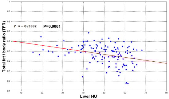
Figure 14.
The plot of TFR vs. liver mean HU values.

Figure 15.
The plot of SFR vs. liver mean HU values.
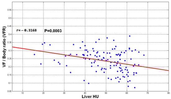
Figure 16.
The plot of VFR vs. liver mean HU values.
The direction of the slope of the line in Figure 14, Figure 15 and Figure 16 indicates that there is a negative correlation between the mentioned observations, which means that when the fate ratios increase in a subject, the HU value decreases since liver density is inversely related to liver fat accordingly. However, the degree of the slope of the red line shows that the correlation is not strong. The obtained results indicate that the accumulation of fat inside the abdomen cavity and the accumulation of the abdomen fat can be linked to the level of liver diffused fat. From the results, it can be said that the accumulation of abdomen fat is not the main reason for increasing the level of diffused fat in the liver. However, it helps to somehow develop the process of increasing that level.
NAFLD is considered a manifestation of metabolic syndrome. It is not surprising that NAFLD is common in the Asia–Pacific region. Estimates of current prevalence range from 5% to 30%, depending on the population studied [28]. By reviewing Table 1, it can be noticed that there is some similarity between the results of the research in that table and the results obtained in this study.
10. Conclusions
A correlation between the abdomen fat ratios and the level of diffused fat in the liver is presented in this research. Data sets of 125 subjects were employed in this research. A negative medium correlation between the TFR and VFR on one side, and the level of diffused fat in the liver on the other side, was found. These correlations were found to be significant. On the other hand, the obtained results show that there is a weak, negative, and insignificant correlation between the SFR ratio and the liver HU mean. This study suggests a direct association between VF and liver fat content. The findings of this study provide further evidence of the effect of abdominal obesity on the health of the liver. The obtained results show that the accumulation of abdomen fat (especially the VF) helps to somehow develop the process of increasing the level of the diffused fat in the liver; this may lead to inflammation of the liver, which is a very serious condition.
Author Contributions
Conceptualization, Y.G., A.A. and A.A.A.; Formal analysis, A.A. and A.A.A.; Funding acquisition, Y.G. and A.M.; Investigation, Y.G. and A.A.; Methodology, Y.G., A.A. and A.M.; Project administration, Y.G.; Resources, A.A.; Software, A.A.; Supervision, Y.G.; Validation, A.A.; Visualization, A.A., A.A.A. and A.M.; Writing—original draft, Y.G., A.A. and A.A.A.; Writing—review & editing, Y.G. and A.A. All authors have read and agreed to the published version of the manuscript.
Funding
This research study has been funded by the Deanship of Scientific Research, Vice Presidency for Graduate Studies and Scientific Research, King Faisal University, Saudi Arabia, under Project AN000372.
Institutional Review Board Statement
Not applicable.
Informed Consent Statement
Not applicable.
Data Availability Statement
The dataset used in this study an in-house dataset(private).
Acknowledgments
This work was supported by the Deanship of Scientific Research, Vice Presidency for Graduate Studies and Scientific Research, King Faisal University, Saudi Arabia, under Project AN000372.
Conflicts of Interest
The authors declare no conflict of interest.
References
- Orville, G.K.; Jonathan, I.; Mark, S.; Jerrold, M.O. Mechanisms of Insulin Resistance in Human Obesity evidence for receptor and post receptor defect. Am. Soc. Clin. Investig. 1980, 65, 1272–1284. [Google Scholar]
- Cristina, L.C.; Timothy, G.W. Diet, Insulin Resistance, and Obesity: Zoning in on Data for Atkins Dieters Living in South Beach. J. Clin. Endocrinol. Metab. 2004, 89, 4197–4205. [Google Scholar]
- Mark, O.G.; Stephen, E.; Sidney, C.P.; Robert, I.J.; Stanley, G.K. Relative Impact of Insulin Resistance and Obesity on Cardiovascular Risk Factors in Polycystic Ovary Syndrome. Metabolism 2003, 52, 713–719. [Google Scholar]
- Claire, M.S.; Mitchell, A.L. Resisting and obesity-associated insulin resistance. Trends Endocrinol. Metab. 2002, 13, 18–23. [Google Scholar]
- Jakobsen, M.U.; Berentzen, T.; Sørensen, T.I.; Overvad, K. Abdominal obesity and fatty liver. Epidemiol. Rev. 2007, 29, 77–87. [Google Scholar] [CrossRef]
- Hamer, O.W.; Aguirre, D.A.; Casola, G.; Lavine, J.E.; Woenckhaus, M.; Sirlin, C.B. Fatty Liver: Imaging Patterns and Pitfalls. RadioGraphics 2006, 26, 1637–1653. [Google Scholar] [CrossRef]
- Ricci, C.; Longo, R.; Gioulis, E.; Bosco, M.; Pollesello, P.; Masutti, F.; Croce, L.S.; Paoletti, S.; de Bernard, B.; Tiribelli, C.; et al. Noninvasive in vivo quantitative assessment of fat content in human liver. J. Hepatol. 1997, 27, 108–113. [Google Scholar] [CrossRef]
- Johnston, R.J.; Stamm, E.R.; Lewin, J.M.; Hendrick, R.E.; Archer, P.G. Diagnosis of fatty infiltration of the liver on contrast enhanced CT: Limitations of liver-minus-spleen attenuation difference measurements. Abdom. Imaging 1998, 23, 409–415. [Google Scholar] [CrossRef]
- Jacobs, J.E.; Birnbaum, B.A.; Shapiro, M.A.; Langlotz, C.P.; Slosman, F.; Rubesin, S.E.; Horii, S.C. Diagnostic criteria for fatty infiltration of the liver on contrast-enhanced helical CT. Am. J. Roentgenol. 1998, 171, 659–664. [Google Scholar] [CrossRef]
- Bydder, G.M.; Chapman, R.W.; Harry, D.; Bassan, L.; Sherlock, S.; Kreel, L. Computed tomography attenuation values in fatty liver. J. Comput. Tomogr. 1981, 5, 33–35. [Google Scholar] [CrossRef]
- Kodama, Y.; Ng, C.S.; Wu, T.T.; Ayers, G.D.; Curley, S.A.; Abdalla, E.K.; Vauthey, J.N.; Charnsangavej, C. Comparison of CT Methods for Determining the Fat Content of the Liver. AJR Am. J. Roentgenol. 2007, 188, 1307–1312. [Google Scholar] [CrossRef]
- Nugent, C.; Younossi, Z.M. Evaluation and management of obesity-related nonalcoholic fatty liver disease. Nat. Clin. Pract. Gastroenterol. Hepatol. 2007, 4, 432–441. [Google Scholar] [CrossRef]
- Dâmaso, A.R.; do Prado, W.L.; de Piano, A.; Tock, L.; Caranti, D.A.; Lofrano, M.C.; Carnier, J.; Cristofalo, D.J.; Lederman, H.; Tufik, S.; et al. Relationship between nonalcoholic fatty liver disease prevalence and visceral fat in obese adolescents. Dig. Liver Dis. 2008, 40, 132–139. [Google Scholar] [CrossRef]
- Jang, S.; Lee, C.H.; Choi, K.M.; Lee, J.; Choi, J.W.; Kim, K.A.; Park, C.M. Correlation of fatty liver and abdominal fat distribution using a simple fat computed tomography protocol. World J. Gastroenterol. 2011, 17, 3335–3341. [Google Scholar] [CrossRef]
- Van Der Poorten, D.; Milner, K.L.; Hui, J.; Hodge, A.; Trenell, M.I.; Kench, J.G.; London, R.; Peduto, T.; Chisholm, D.J.; George, J. Visceral Fat: A Key Mediator of Steatohepatitis in Metabolic Liver Disease. Hepatology 2008, 48, 49–457. [Google Scholar] [CrossRef]
- de Barros, F.; Setúbal, S.; José, M.M.; Loraine, F.; Andressa, G. Correlation of non-alcoholic fatty liver disease and features of metabolic syndrome in morbidly obese patients in the preoperative assessment for bariatric surgery. ARQ Brasileiros Cir. Dig. 2016, 29, 260–263. [Google Scholar] [CrossRef]
- Kim, C.H. Measurements of Adiposity and Body Composition. Korean J. Obes. 2016, 25, 115–120. [Google Scholar] [CrossRef]
- Yki-Jarvinen, H. Fat in the liver and insulin resistance. Ann. Med. 2005, 37, 347–356. [Google Scholar] [CrossRef]
- Ahmed, M.M.; Abdul Rahman, R.; Syamsiah, M.; Rozi, B.M. Survey on liver CT image segmentation methods. Artif. Intell. Rev. 2012, 37, 83–95. [Google Scholar]
- Tohru, Y.; Tadashi, N.; Mitsukazu, Y.; Abdul, M.; Masakazu, H.; Kouichi, Y.; Takeshi, A.; Kazuaki, K.; Tohru, F.; Shizuya, Y.; et al. Abdominal fat: Standardized technique for measurement at CT. Radiology 1999, 211, 283–286. [Google Scholar]
- Romero, D.; Ramirez, J.C.; Marmol, A. Quantification of subcutaneous and visceral adipose tissue using CT. In Proceedings of the IEEE International Workshop on Medical Measurements and Applications, Benevento, Italy, 20–21 April 2006; pp. 128–133. [Google Scholar]
- Zhou, X.; Hara, T.; Fujita, H.; Yokoyama, R.; Kiryu, T.; Kanematsu, M.; Hoshi, H. Preliminary Study for Automated Recognition of Anatomical Structure from Torso CT images. In Proceedings of the 2005 IEEE Engineering in Medicine and Biology 27th Annual Conference, Shanghai, China, 17–18 January 2006; pp. 650–653. [Google Scholar]
- Pednekar, A.; Bandekar, A.N.; Kakadiaris, I.A.; Naghavi, M. Automatic Segmentation of Abdominal Fat from CT Data. In Proceedings of the 2005 Seventh IEEE Workshops on Applications of Computer Vision (WACV/MOTION’05), Breckenridge, CO, USA, 5–7 January 2005; Volume 1, pp. 308–315. [Google Scholar]
- Ahmed, A.; Ghassan, A.H. Automatic liver segmentation method using non-contrast enhanced CT images for liver fat evaluation by Matlab. Int. J. Adv. Trends Comput. Sci. Eng. 2017, 6, 40–50. [Google Scholar]
- Dunn, J.C. A Fuzzy Relative of the ISODATA Process and Its Use in Detecting Compact Well-Separated Clusters. J. Cybern. 1973, 3, 32–57. [Google Scholar] [CrossRef]
- Bezdek, J.C. Pattern Recognition with Fuzzy Objective Function Algorithms; Plenum Press: New York, NY, USA, 1981. [Google Scholar]
- Otsu, N. A threshold selection method from gray-level histograms. IEEE Trans. Syst. Man Cybern. 1979, 9, 62–66. [Google Scholar] [CrossRef]
- Amarapurkar, D.N.; Hashimoto, E.; Lesmana, L.A.; Sollano, J.D.; Chen, P.J.; Goh, K.L. How common is non-alcoholic fatty liver disease in the Asia–Pacific region and are there local differences? J. Gastroenterol. Hepatol. 2007, 22, 788–793. [Google Scholar] [CrossRef]


Publisher’s Note: MDPI stays neutral with regard to jurisdictional claims in published maps and institutional affiliations. |
© 2022 by the authors. Licensee MDPI, Basel, Switzerland. This article is an open access article distributed under the terms and conditions of the Creative Commons Attribution (CC BY) license (https://creativecommons.org/licenses/by/4.0/).