Measurements and Correctness Criteria for Determining the Line Length of the Data Image Obtained in the Process of Electromagnetic Infiltration

Abstract

The protection of information against electromagnetic penetration is one of the most important aspects related to the protection of information against its non-invasive acquisition. Compared to the activities of cybercriminals, the use of electromagnetic emissions in the electromagnetic infiltration process does not leave any traces of activity, and the owner of the information is not aware of its loss. The most common activities of electromagnetic eavesdropping are related to the infiltration of emission sources, graphically revealing the processing of information using both analog and digital methods. This allows for the presentation of reconstructed data in the form of images. Correct display of the acquired information requires knowledge of raster parameters such as line length and the number of lines building the reconstructed image. Due to the lack of direct access to the intercepted device, knowledge in this field does not allow for the correct determination of the aforementioned parameters, and thus, for recreating an image that would contain legible and understandable data. Additionally, incorrect values of the parameters result in failure of further processing of the obtained image, e.g., by using a coherent summation of images. Therefore, it is necessary to propose a solution that will allow not so much to roughly define the raster parameters but to estimate them precisely. Moreover, it should enable the automation of the process after the implementation of an appropriate algorithm. The article proposes an algorithm for estimating the line length of the reconstructed image. The raster parameter estimated with the use of the algorithm allows for summarizing images several dozen times with a significant improvement in the image quality and readability of the data contained in it. The image summation algorithm is very often used as one of the main image processing methods in the electromagnetic infiltration process. Incorrect raster parameters often make coherent summation useless. The proposed algorithm for estimating the line length of the reconstructed image uses three methods of determining the line length of the image for a given accuracy. At the same time, criteria were indicated that must be met to determine the correct length of the image line for the assumed accuracy of estimation. Obtained results confirmed that the proposed methods and criteria are effective in the process of electromagnetic infiltration. These methods allow us to determine the line length of reconstructed images with accuracy up to ${10}^{-5}$.

1. Introduction

Information protection is one of the aspects of everyday human life. When processing information, particular attention is paid to network security [1,2], security of data processed in paper form, or protection of data carriers held [3]. It should be noted, however, that data processing (e.g., printing, displaying) occurring in electronic form poses a great risk related to the loss of this data in a non-invasive manner [4,5,6]. The reason for such a phenomenon is the formation of electromagnetic emissions, the distinctive features of which may allow the reconstruction of protected data [7,8,9,10].

The hazards related to the formation of electromagnetic revealing emissions are analyzed primarily in terms of the sources of these emissions in the graphic tracks. This is due to the possibility of direct presentation of the obtained information in the form of images containing the processed data. In particular, the sources of such emissions may be computer monitors, displays of multifunction devices or in a simpler form—displays of laser printers, graphic layouts of printing devices, and all kinds of data displays [11,12,13,14].

The process of non-invasive data acquisition based on electromagnetic emissions does not end with sampling and recording such signals. In order to display the information properly, the correct raster parameters are necessary, i.e., the length of the horizontal line of the reconstructed image and the number of lines (image height) making up a given image. These parameters should be consistent with the parameters of the original image [15,16,17,18].

The issue related to the determination of raster parameters can be considered in several variants. The first is laboratory tests. During such tests, personnel can access the infiltrated device [19,20,21,22,23]. However, depending on the device under test, knowing the parameters of the displayed image may not be obvious. While in the case of computer monitors it is not too difficult, in the case of other displays, e.g., multifunction devices, the process of getting to know the display’s operating mode can be a big problem. The second variant is the study of an unknown object. This concerns operational activities under real conditions. Then it is not possible to know the raster parameters, even of a typical computer monitor. The determination of the value of these parameters must be supported by appropriate algorithms that will allow for the automation of the process [24,25,26,27,28,29].

Many publications applying to the electromagnetic infiltration process and the non-invasive acquisition of information present the analysis of threats related to the above-mentioned phenomenon and the possibilities of data recovery based on the recorded signals of revealing emissions [30,31,32,33]. In these publications solutions that can effectively protect data against electromagnetic infiltration are presented. In the case of sources of revealing emissions in the form of graphic paths, the analyzes performed are based on images that give the impression of being “aligned”, i.e., for the correct value of the image line length. There is no mention of how this value was estimated and with what accuracy. The most important issue is to visualize the obtained data and show the reader the essence of the threat.

The article presents the possibilities of determining the length of the horizontal line of the image for the case defined as operational activities, i.e., the lack of knowledge of the geometrical parameters of the reconstructed image. The starting point is a rough determination of the image line length on the basis of, for example, the analysis of the emission signal in the time or frequency domain, e.g., the Chirp-Z transform [34,35]. This is possible due to the periodic repetition of characteristic image elements in the aforementioned waveform. These are, for example, pulses correlated with the horizontal synchronization signal of a computer monitor.

Rough determination of the value of the image length line $d_{\mathsf{\Delta }}$ (image width) allows us to start the activities related to the line length estimation with the given accuracy Δ, starting from ${10}^0$ and ending e.g., at ${10}^{-5}$. Practice shows that the accuracy at the level of ${10}^{-5}$ allows for a significant improvement in the quality of the reconstructed image for a 30–100-fold summation of $Su{m}_{MTL}$ of the replicas of the images obtained from the recorded emission signal revealing $s\left(t\right)$. There remains the question of what measures and their criteria should be adopted, which would allow us to determine the correct value of the length $d_{\mathsf{\Delta }}$ of the image line, allowing for effective summation of image replicas. Effective summation is understood as a process that allows us to improve the image quality assessed, among others, by visual analysis and allowing to increase the value of the signal-to-noise ratio parameter described by the formula:

$$SNR=10\log \left(\frac{Signal\_power}{Noise\_power}\right).$$

(1)

Initial considerations concerned the analysis of the possibility of using selected methods of assessing the contrast of digital images, based on the value of the average amplitude of the image pixels, on the maximum and minimum values of the image pixel amplitude, and the variance of gray levels [36,37]. Each of the methods is described by Equations (2), (8), and (11), respectively.

• (a) evaluation of the contrast based on the value of the average amplitude of pixels of the reconstructed image

  $$Contras{t}_{I\_\_Un}=\frac{Contras{t}_{I\_\mathsf{\Delta }}}{maximu{m}_{I\_\mathsf{\Delta }}},$$

  (2)

  where:

  $$Contras{t}_{I\_\mathsf{\Delta }}=\frac{l_{\mathsf{\Delta }\_max}-l_{\mathsf{\Delta }\_min}}{\overline{l_{\mathsf{\Delta }}}},$$

  (3)

  $$maximu{m}_{I\_\mathsf{\Delta }}=\max \left(Contras{t}_{I\_\mathsf{\Delta }}\right),$$

  (4)

  $$\overline{l_{\mathsf{\Delta }}}=\frac{1}{N·M}{\displaystyle \sum }_{m=0}^{M-1}{\displaystyle \sum }_{n=0}^{N-1}{l}_{\mathsf{\Delta }}\left(n,m\right),$$

  (5)

  $$l_{\mathsf{\Delta }\_\max }=\underset{n,m}{\max }\left(l_{\mathsf{\Delta }}\left(n,m\right)\right),$$

  (6)

  $$l_{\mathsf{\Delta }\_min}=\underset{n,m}{\min }\left(l_{\mathsf{\Delta }}\left(n,m\right)\right),$$

  (7)
  $M$—columns number of reconstructed image;
  $m$—number of column of reconstructed image ($m=$ 0, 1, 2, …, $M-1$);
  $N$—rows number (lines) of reconstructed image;
  $n$—number of row (line) of reconstructed image ($n=$ 0, 1, 2, …, $N-1$);
  $\mathsf{\Delta }$—accuracy of the line length $d_{\mathsf{\Delta }}$ estimation of the reconstructed image for which the contrast of the reconstructed image is calculated. In the carried out analyzes, $\mathsf{\Delta }=1.0$, 0.1, 0.01, 0.001, 0.0001 and 0.00001 were assumed;
  $l_{\mathsf{\Delta }}$—value of image pixel amplitude for the line length $d_{\mathsf{\Delta }}$ calculated for accuracy ∆;
  $l_{\mathsf{\Delta }\_max}$—the maximum value of the image pixel amplitude for the line length $d_{\mathsf{\Delta }}$ calculated for the accuracy ∆;
  $l_{\mathsf{\Delta }\_min}$—the minimum value of the image pixel amplitude for the line length $d_{\mathsf{\Delta }}$ calculated for the accuracy ∆.
• (b) evaluation of the contrast based on the maximum and minimum values of the amplitude of the pixel of the reconstructed image

  $$Contras{t}_{II\_\mathsf{\Delta }\_Un}=\frac{Contras{t}_{II\_\mathsf{\Delta }}}{maximu{m}_{II\_\mathsf{\Delta }}},$$

  (8)

  where:

  $$Contras{t}_{II\_\mathsf{\Delta }}=\frac{l_{\mathsf{\Delta }\_max}-l_{\mathsf{\Delta }\_min}}{l_{\mathsf{\Delta }\_max}+l_{\mathsf{\Delta }\_min}},$$

  (9)

  $$maximu{m}_{II\_\mathsf{\Delta }}=\max \left(Contras{t}_{II\_\mathsf{\Delta }}\right),$$

  (10)
• (c) evaluation of the contrast based on the variance of the gray levels of the reconstructed image

  $$Contras{t}_{III\_\mathsf{\Delta }\_Un}=\frac{Contras{t}_{III\_\mathsf{\Delta }}}{maximu{m}_{III\_\mathsf{\Delta }}},$$

  (11)

  where:

  $$Contras{t}_{III\_\mathsf{\Delta }}=\frac{4}{M·N·{255}^2}{\displaystyle \sum }_{m=0}^{M-1}{\displaystyle \sum }_{n=0}^{N-1}{\left[l_{\mathsf{\Delta }}\left(i,j\right)-\overline{l_{\mathsf{\Delta }}}\right]}^2,$$

  (12)

  $$maximu{m}_{III\_\mathsf{\Delta }}=\max \left(Contras{t}_{III\_\mathsf{\Delta }}\right),$$

  (13)

The results of preliminary analyzes of the above methods showed that they are not suitable for the specific conditions related to the images reconstructed in the process of electromagnetic infiltration [38,39,40,41]. Changing the length $d_{\mathsf{\Delta }}$ of the line does not change the pixel amplitude values of the image. Thus, the values calculated according to the Equations (2), (8), and (11) do not change or change slightly as a function of changes in the value of parameter $d_{\mathsf{\Delta }}$. The reasons for this phenomenon should be sought in the consistency of image quality as a function of changes in the line length of the image. However, appropriate calculations (in accordance with the relationships (2), (8), and (11)) of the contrast value for selected images obtained from the recorded revealing emission signals were performed. The maximum contrast value was adopted as the criterion for the correctness of determining the length $d_{\mathsf{\Delta }}$ of the image line.

Since the contrast assessment methods do not meet the requirements for estimating the $d_{\mathsf{\Delta }}$ parameter, the author’s proposed methods allow for effective estimation of the $d_{\mathsf{\Delta }}$ line length of the reconstructed image based on the analysis of the amplitude values of the pixels building the image for individual image columns. In this way, the assessment of minimizing the deviation of the graphic elements of the image from the vertical is made.

In summary, our contributions to this work are three-fold:

• the showing that the methods of contrast assessment are not effective in relation to reconstructed images in the process of electromagnetic penetration;
• the proposing three methods which allow for determining the correct line length of the reconstructed image;
• the possibility of using the proposed methods in the automatic process of line length determining.

The rest of this article is organized as follows. The second section introduces the process of sampling and recording revealing emission signals and why this process has an influence on the necessity of line length determining reconstructed images. Section 3 details the proposed methods of determining and evaluating raster parameters. In Section 4 the test images and the test conditions were described. In Section 5, the experimental results and corresponding analyses are provided, and some conclusions are made in Section 6.

2. Sampling and Recording of Revealing Emission Signals

In the electromagnetic infiltration process, the case of revealing emission signals having the character of video signals is particularly interesting [42,43,44,45,46,47,48,49]. In many devices, the raster technique is used to visualize graphic information (monitors, printers, operator panels). It consists in transforming a one-dimensional signal (samples of the information signal) into a two-dimensional matrix, the cells of which will contain data on the luminance and chrominance of the image being created. The correctness of the representation is ensured by the knowledge of its geometrical dimensions, i.e., the length $d_{\mathsf{\Delta }}$ and the number of lines. Knowing the line length of the image is especially important. Assuming an incorrect value of this parameter leads to distortions, visible as a characteristic tilt of the image elements (Figure 1).

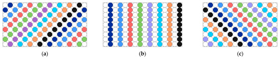
Figure 1. Image reconstructed for the correct value of the line length (b), the line length value too large (a), the line length value too small (c).

Figure 1 shows the case of an image consisting of alternately arranged white and colored balls. In the case of the correct value of the line length (Figure 1b) obtained image consists of vertical lines with a specific color. Each deviation from this value causes the lines to slope to the left (too high value, Figure 1a) or the right (too low value, Figure 1c).

In the case of reconstructing images from recorded revealing signals, the correct, exact value of the image line length in the general case is unknown. When analyzing the course of the image reconstruction (rasterization) process, it can be noticed that it consists in transforming the one-dimensional revealing emission signal, i.e., a set of samples of its amplitude value, into a two-dimensional matrix with a size strictly defined by the raster parameters (number and length of image lines). The numerical value of each sample placed in a matrix corresponding to these sizes is interpreted as the luminance value of a given point of the reconstructed image (Figure 2).

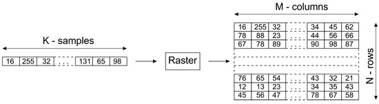
Figure 2. An operation mechanism of image reconstruction (raster).

In the case of revealing emission signals, for which the level of the useful signal significantly exceeds the level of the accompanying noise, i.e., the signal-to-noise ratio $SNR\gg 0$, even incorrect reconstruction of the image allows for the data included in this image to be used for the identification of the revealing emission signal. However, for highly noisy signals, information related to them under such conditions may be lost. The improvement of the output $SNR$ can be obtained by using the image summation method, i.e., coherent summation in the time domain. However, its use requires precise determination of the parameters of summed images. Their desynchronization leads to the summation of random points of the corresponding matrix and, consequently, the blurring of the information contained in them. This problem is illustrated in (Figure 3, Figure 4 and Figure 5), where the effects of the signal taken from the RED line of the VGA (Video Graphics Array) interface operating with a resolution of 640 × 480/60 Hz are presented. The signal sampling frequency was 62.5 MHz. Under such conditions, the correct length $d_{\mathsf{\Delta }}$ of the line is approx. 1984.11007 (Figure 3); assuming the value of 1985 causes image geometry distortions (Figure 4), which in the case of summation operations causes its complete blurring (Figure 5).

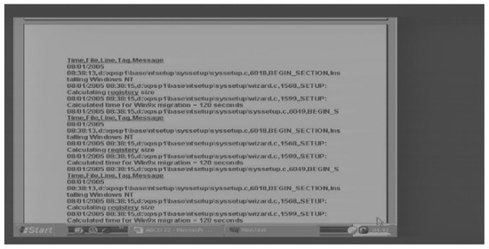
Figure 3. The reconstructed image (rasterized) in correct way, VGA interface signal as a source of reveal emission, 640 × 480/60 Hz mode, 62.5 MHz sampling rate, line length 1984.11007.

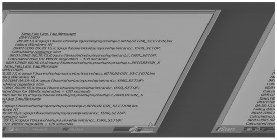
Figure 4. The reconstructed image (rasterized) in incorrect way, VGA interface signal as a source of reveal emission, 640 × 480/60 Hz mode, 62.5 MHz sampling rate, line length 1985.

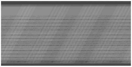
Figure 5. The reconstructed image (rasterized) in incorrect way, VGA interface signal as a source of reveal emission, 640 × 480/60 Hz mode, 62.5 MHz sampling rate, line length 1985, summed 10 times.

Due to the finite accuracy of performance of the components of video systems of IT devices, the values of the synchronization parameters of images reconstructed from the revealing emission signals from video monitors may significantly, in the context of coherent summation requirements, differ from the catalog data defined by the VESA (Video Electronics Standards Association) guidelines [50], and even they can differ from one instance to the next of the same type of device. In addition, in the case of devices such as laser printers, the course of the printing process depends on other factors related to the operating conditions of the device, such as the current temperature of the printing system or the type of paper. Due to these factors, each attempt to recreate an image from the recorded revealing emission signal requires the determination of its imaging parameters. This determination can be made by the trial and error method, matching the appropriate values on a database of the catalog or archive data from previous surveys. However, these activities are labor-intensive and also require some experience from the operator.

Video signals processed in the tracks of monitors, laser printers, or displays have a strictly defined time structure. In the case of screen monitors, both the VGA and DVI/HDMI standards (Digital Video Interface/High-Definition Multimedia Interface) maintain the principles of the so-called framing of images. Based on the information contained in [50], it is possible to provide the most important raster parameters of the screen for selected operating modes (Table 1).

Table 1. Nominal parameters for selected graphic modes according to VESA [50].

Operating Mode of Display	Total Number of Image Lines	Total Number of Pixels in Line	Pixel Frequency [MHz]	Horizontal Sync Frequency [kHz]
640 × 480/60 Hz	525	800	25.175	31.500
800 × 600/60 Hz	628	1056	40.000	37.789
1024 × 768/60 Hz	806	1344	65.000	48.363
1280 × 1024/60 Hz	1066	1688	108.000	63.981
1366 × 768/60 Hz	798	1792	85.500	47.712
1440 × 900/60 Hz	934	1904	106.500	55.935
1600 × 900/60 Hz	1000	1800	108.000	60.000
1600 × 1200/60 Hz	1250	2160	162.000	75.000
1920 × 1080/60 Hz	1125	2200	148.500	67.500
2048 × 1152/60 Hz	1200	2250	162.000	72.000
4096 × 2160/60 Hz	2222	4176	556.744	133.320

It is worth noting that the frequency values given in Table 1 are nominal values that define the mode according to the VESA standard. The formulas defining the exact values of these parameters and the values of the constants necessary to determine them can be found in [51]. Due to the finite accuracy of the components that make up the synchronization signal generation circuits, the actual values of their frequencies for specific graphics card systems may differ from the nominal ones. It is not always possible to directly measure the parameters of video signals in lines of graphic interfaces. For the above reasons, it is impossible to properly reconstruct an image based on catalog values.

In addition, during the recording of the real revealing emission signals using a physical analog-to-digital converter (DAC), only specific signal sampling frequency values can be used. For example, the 8-bit PDA-1000 converter card produced by Signatec, used in the Electromagnetic Compatibility Laboratory of the Military Communication Institute-State Research Institute (EMC Laboratory of MCI-SRI), offers a maximum sampling rate of $1 GS/s$, which may be reduced as a result of the application of card clock frequency division in the range from 2 to 1024.

Assuming the perfect execution of both the transducer card and the graphics card elements, and assuming that the minimum sampling frequency should be at least equal to the “pixel frequency” value, for the previously selected monitor operation modes there are obtained appropriate (estimated) values of parameters of acquisition and rasterization of emission signals revealing (Table 2).

Table 2. Nominal raster parameters for sampling signals.

Operating Mode of Display	Pixel Frequency [MHz]	Sampling Rate [MHz]	Vertical Synchronization Frequency [kHz]	Estimated Number of Pixels on the Line
640 × 480/60 Hz	25.175	31.25	31.500	992.063492
800 × 600/60 Hz	40.000	62.50	37.789	1653.920453
1024 × 768/60 Hz	65.000	125.00	48.363	2584.620474
1280 × 1024/60 Hz	108.000	125.00	63.981	1953.705006
1366 × 768/60 Hz	85.500	125.00	47.712	2619.885983
1440 × 900/60 Hz	106.500	125.00	55.935	2234.736748
1600 × 900/60 Hz	108.000	125.00	60.000	2083.333333
1600 × 1200/60 Hz	162.000	250.00	75.000	3333.333333
1920 × 1080/60 Hz	148.500	250.00	67.500	3703.703704
2048 × 1152/60 Hz	162.000	250.00	72.000	3472.222222
4096 × 2160/60 Hz	556.744	1000.00	133.320	7500.750075

The information provided in Table 2 shows that in the case of the rasterization of the signal obtained by sampling with the use of an ADC converter card, the line length of the reconstructed image is not expressed by the total number of pixels, which must be taken into account in the image reconstruction algorithm. In addition, the accuracy of reproducing this value is important in the process of coherent image summation. The experience of the EMC Laboratory of MCI-SRI shows that in this case the value should be determined with an accuracy of at least ${10}^{-4}$. Figure 6 shows a comparison of the effect of summing images (30 times) with an accuracy of 0.001. The image signal was obtained by reading the luminance values from the *.bmp file mapping the so-called Word editor screenshot for the 1920×1080 monitor; the correct image line length was 1920 pixels.

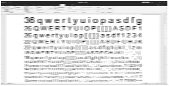
Figure 6. Image reconstructed by summing 30 images for the line length $d=1920.001$.

Observing the effect of the summation operation, one can notice a clear effect of desynchronization of the replicas of the image caused by the insufficient accuracy of reproducing the length of its lines (image width).

3. Evaluation of Raster Parameters

The quality of the reconstructed image can be assessed on the basis of both subjective (observational) and objective (computational) methods. Each of them gives a result that may be acceptable in the process of reading the graphic data contained in the reconstructed images. However, reading the data does not always end further image processing. Very often the images contain a number of disturbances that should be eliminated using various methods. One of them is the coherent summation of several realizations of the same image. In this case, the evaluation result of the subjective quality of the reconstructed single image very often becomes insufficient for the effectiveness of the coherent summation method in improving the quality of the reconstructed image. The reason is incorrectly determined raster parameters, i.e., the length of the image lines and the number of lines forming the image. In this case, computational metrics or objective methods may prove useful.

The authors proposed three different methods to estimate the line length of the reconstructed image. The effectiveness of each of the methods was demonstrated on the basis of the analyzes carried out with the use of the recorded actual revealing emission signals, the sources of which were test images showing various structures of the processed data.

Each of the proposed methods is based on the input data $D_{Ent}$, which is the initial value of the line length of the image. It is assumed that the $D_{Ent}$ value of the image line length d is indicated by a prior analysis that uses the Chirp-Z transform algorithm or the periodicity analysis of the recorded revealing emission signal [52,53]. At a later stage, it is necessary to estimate the $d_{\mathsf{\Delta }}$ parameter more precisely. This process begins with the estimation of the $d_{\mathsf{\Delta }}$ value with the accuracy of $\mathsf{\Delta }=1.0$. For this purpose, the values of the proposed measures are calculated for methods I, II, and III, for the length $d_1$ of the line according to the relationship:

$$d_{\mathsf{\Delta }}=D_{Ent}-\left(10·\mathsf{\Delta }-n·\mathsf{\Delta }\right)$$

(14)

where:

$\mathsf{\Delta }=1.0$;

$n=0,1,2,\dots ,20$;

$D_{Ent}$—image line length value estimated according to a previous step (e.g., Chirp-Z transform).

Meeting the criteria for the proposed measures allows to estimate the length $d_{\mathsf{\Delta }}$ of the line for a given accuracy. Then the accuracy of the estimation is increased according to the relationship:

$$d_{\mathsf{\Delta }}=d_{\mathsf{\Delta }·10}-\left(10·\mathsf{\Delta }-n·\mathsf{\Delta }\right)$$

(15)

where:

$\mathsf{\Delta }$—the accuracy of the image line length estimation.

$d_{\mathsf{\Delta }\mathsf{\Delta }10}$—the line length estimated with a given accuracy Δ meeting the adopted criterion defined below.

Meeting the appropriate criterion allows to indicate one of the $d_{\mathsf{\Delta }}$ values calculated in the interval $\left[d_{\mathsf{\Delta }·10}-10·\mathsf{\Delta };d_{\mathsf{\Delta }·10}+10·\mathsf{\Delta }\right]$.

Three methods have been proposed:

• (a) method I—based on the minimum value of the sum of the differences between the maximum and minimum amplitudes calculated for the individual vertical lines of the reconstructed image.
• (b) method II—based on the maximum value of the difference of the maximum and minimum values of the sum of the pixel amplitudes calculated for the individual vertical lines of the reconstructed image.
• (c) method III—based on the minimum value of the sum of the maximum pixel amplitudes calculated for the individual vertical lines of the reconstructed image.

For each of the methods, a criterion was adopted related to the achievement of the required value by the calculated quantity. In the case of methods, I and III, it is the minimum calculated for the $d_{\mathsf{\Delta }}$ value determined by relations (14) and (15) for the given accuracy Δ, while for method II it is the maximum for analogous conditions.

3.1. Method I—Based on the Minimum Value of the Sum of the Differences between the Maximum and Minimum Amplitudes Calculated for the Individual Vertical Lines of the Reconstructed Image

The method requires the calculation of the $d_{\mathsf{\Delta }}$ value for the given accuracy Δ, for which the maximum $Maximum\_d_{\mathsf{\Delta }}$ and the minimum $Minimum\_d_{\mathsf{\Delta }}$ pixel amplitude values are calculated for each $m$ column of the reconstructed image according to the formula:

$$Maximum\left(d_{\mathsf{\Delta }},m\right)=\underset{n}{\max }\left(Maximum\left(d_{\mathsf{\Delta }},n\right)\right),$$

(16)

$$Minimum\left(d_{\mathsf{\Delta }},m\right)=\underset{n}{\min }\left(Minimum\left(d_{\mathsf{\Delta }},n\right)\right),$$

(17)

$m=0,1,2,\dots ,M$—column number of reconstructed image

$n=0,1,2,\dots ,N$—row (line) number of reconstructed image.

Then the sum of the differences $Maximum\_d_{\mathsf{\Delta }}\left(m\right)-Minimum\_d_{\mathsf{\Delta }}\left(m\right)$ is determined:

$$Su{m}_{Met\_I}\left(d_{\mathsf{\Delta }}\right)={\displaystyle \sum }_{m=0}^{M-1}\left(Maximum\_d_{\mathsf{\Delta }}\left(m\right)-Minimum\_d_{\mathsf{\Delta }}\left(m\right)\right),$$

(18)

which is calculated independently for each $d_{\mathsf{\Delta }}$ value for the given accuracy Δ. In the next step, the maximum value $Su{m}_{Met\_I}\left(d_{\mathsf{\Delta }}\right)$ is determined:

$$Maximum\_Su{m}_{Met\_I}=\underset{d_{\mathsf{\Delta }}}{\max }\left(Su{m}_{Met\_I}\left(d_{\mathsf{\Delta }}\right)\right)$$

(19)

which allows to calculate the normalized value:

$$Sum\_mi{n}_{Met\_I\_Un}\left(\mathsf{\Delta }\right)=\underset{d_{\mathsf{\Delta }}}{\min }\left(\frac{Su{m}_{Met\_I}\left(d_{\mathsf{\Delta }}\right)}{Maximum\_Su{m}_{Met\_I}}\right).$$

(20)

The minimum value determined by the relationship (20) is assumed as the criterion for determining the proper length $d_{\mathsf{\Delta }}$ of the image line for the given accuracy.

3.2. Method II—Based on the Maximum Value of the Difference of the Maximum and Minimum Values of the Sum of the Pixel Amplitudes Calculated for the Individual Vertical Lines of the Reconstructed Image

Method II is not based directly on the maximum and minimum amplitude values of the pixels building the reconstructed image. Relevant maximum values $Maximu{m}_{Met\_II}\left(d_{\mathsf{\Delta }}\right)$ and minimum $Minimu{m}_{Met\_II}\left(d_{\mathsf{\Delta }}\right)$ are calculated for the sums of $Su{m}_{Met\_II}\left(d_{\mathsf{\Delta }},m\right)$ pixel amplitude values calculated for each columns of the analyzed image according to the dependencies:

$$Su{m}_{Met\_II}\left(d_{\mathsf{\Delta }},m\right)={\displaystyle \sum }_{n=0}^{N-1}l\left(n,m\right),$$

(21)

$$Maximu{m}_{Met\_II}\left(d_{\mathsf{\Delta }}\right)=\underset{m}{\max }\left(Su{m}_{Met\_II}\left(d_{\mathsf{\Delta }},m\right)\right),$$

(22)

$$Minimu{m}_{Met\_II}\left(d_{\mathsf{\Delta }}\right)=\underset{m}{\min }\left(Su{m}_{Met\_II}\left(d_{\mathsf{\Delta }},m\right)\right),$$

(23)

where:

$l\left(n,m\right)$—pixel amplitude value with coordinates $\left(n,m\right)$.

Then, in accordance to the adopted algorithm, the differences $Di{f}_{Met\_II}\left(d_{\mathsf{\Delta }}\right)$ between the maximum value $Maximu{m}_{Met\_II}\left(d_{\mathsf{\Delta }}\right)$ and the minimum $Minimu{m}_{Met\_II}\left(d_{\mathsf{\Delta }}\right)$ the sums $Su{m}_{Met\_II}\left(d_{\mathsf{\Delta }},m\right)$, according to the formula:

$$Di{f}_{Met\_II}\left(d_{\mathsf{\Delta }}\right)=Maximu{m}_{Met\_II}\left(d_{\mathsf{\Delta }}\right)-Minimu{m}_{Me{t}_{II}}\left(d_{\mathsf{\Delta }}\right).$$

(24)

The next steps of the procedure are the same as in the case of method I and require the determination of the maximum value $Maximu{m}_{Di{f}_{Met\_II}}\left(\mathsf{\Delta }\right)$:

$$Maximu{m}_{Di{f}_{Met\_II}}\left(\mathsf{\Delta }\right)=\underset{d_{\mathsf{\Delta }}}{\max }\left(Di{f}_{Met\_II}\left(d_{\mathsf{\Delta }}\right)\right),$$

(25)

of the difference $Di{f}_{Met\_II}\left(d_{\mathsf{\Delta }}\right)$ determined by the relationship (24), which allows to calculate the normalized value:

$$Di{f}_{Met\_II\_Un}\left(d_{\mathsf{\Delta }}\right)=\frac{Di{f}_{Met\_II}\left(d_{\mathsf{\Delta }}\right)}{Maximu{m}_{Di{f}_{Met\_II}}\left(\mathsf{\Delta }\right)}.$$

(26)

The maximum value determined by the formula (27) is assumed as the criterion for determining the proper length $d_{\mathsf{\Delta }}$ of the image line for the given accuracy:

$$Dif\_ma{x}_{Met\_II\_Un}\left(\mathsf{\Delta }\right)=\underset{d_{\mathsf{\Delta }}}{\max }\left(Di{f}_{Met\_II\_Un}\left(d_{\mathsf{\Delta }}\right)\right).$$

(27)

3.3. Method III—Based on the Minimum Value of the Sum of the Maximum Pixel Amplitudes Calculated for the Individual Vertical Lines of the Reconstructed Image

Method III is similar to method I, requiring only the calculation of the maximum values of $Maximum\_d_{\mathsf{\Delta }}\left(m\right)$ image pixel amplitudes for the $d_{\mathsf{\Delta }}$ values determined for the given accuracy Δ for each column m of the reconstructed image according to the relationship:

$$Su{m}_{Met\_III}\left(d_{\mathsf{\Delta }}\right)={\displaystyle \sum }_{m=0}^{M-1}Maximum\_d_{\mathsf{\Delta }}\left(m\right).$$

(28)

Further stages of the procedure are the same as in the case of method III and require the determination of the maximum value of $Maximum\_Su{m}_{Met\_III}$:

$$Maximum\_Su{m}_{Met\_III}=\underset{d_{\mathsf{\Delta }}}{\max }\left(Su{m}_{Met\_III}\left(d_{\mathsf{\Delta }}\right)\right),$$

(29)

which allows to calculate the normalized value:

$$Sum\_mi{n}_{Met\_III\_Un}\left(\mathsf{\Delta }\right)=\underset{d_{\mathsf{\Delta }}}{\min }\left(\frac{Su{m}_{Met\_III}\left(d_{\mathsf{\Delta }}\right)}{Maximum\_Su{m}_{Met\_III}}\right).$$

(30)

The minimum value determined by the relationship (30) is assumed as the criterion for determining the proper line length $d_{\mathsf{\Delta }}$ of the image for the given accuracy.

4. Test Images and Test Conditions

The measures and criteria for determining the correct length lines $d_{\mathsf{\Delta }}$ of the reconstructed image presented in the previous chapter have been verified on the basis of the actual test results. The results of these tests are the registered revealing emission signals, the source of which were the graphic lines of the computer set and the display of the multifunction device. The test images used in the research and the view of the device display are shown in Figure 7. As test images, there were proposed text data (texts written with different fonts and in different character sizes) and photos showing different views. The variety of test images allowed for a detailed analysis of the proposed measures and criteria in the process of estimating the correct length line $d_{\mathsf{\Delta }}$ of the reconstructed image.

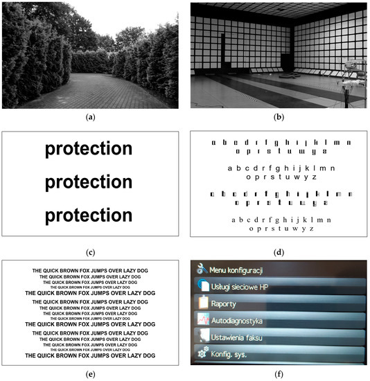
Figure 7. Images displayed on a computer monitor (a–c,e,f) or multifunction device display (d), which are the source of revealing emissions: (a) a photo showing the road along the bushes, (b) a photo of the inside of an anechoic chamber, (c) three words “protection”, letter size 36, Arial font, (d) letter signs written with four fonts Safe Symmetric, Arial, Safe Asymmetric, Times New Roman, (e) a sentence written in Arial font of various sizes of letters, (f) display screen (Configuration menu) of the multifunction device.

The tests of the revealing emission signals, which are the basis for the reconstruction of data in the form of images, for which the process of determining the correct length lines was carried out, were carried out in an anechoic chamber. The measuring test system is shown in Figure 8. The measurement system TEMPEST Test System DSI-1550A and the FSWT26 receiver from Rohde & Schwarz with a set of measurement antennas (a vertical active rod antenna (100 Hz up to 50 MHz), a biconical active antenna (20 MHz up to 200 MHz) and a dipole active antenna (200 MHz up to 1000 MHz)) were used in the tests. The PDA-1000 8-bit analog-to-digital converter card, manufactured by Signatec (PDA100 Scope Application software, version 1.19), was used to sample the revealing emission signals. The card offers a signal sampling rate of 1 GS/s, which may be reduced by using the card clock frequency division in the range from 2 to 1024.

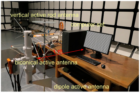
Figure 8. The measuring system of revealing emission signals.

Initial (rough) line length estimation was performed in the Program Raster Generator for the given catalog operating parameters of the test computer monitor (for known parameters). If such parameters are not known-no access to the eavesdropped monitor or for the displays of multifunction devices-their rough estimation can be performed in accordance with the algorithm of the Chirp-Z transform or periodicity analysis of the recorded emission signal of revealing [34,35,52,53]. As previously mentioned, this is the step of roughly determining the line length of the reconstructed image. In the first stage, the line length estimation is performed with accuracy to unity in the vicinity of ±10 around the roughly determined d value of the line length. This means that for $d_1=1087$, the estimation of the value of $d_{\mathsf{\Delta }}$ is carried out in the range from 1077 to 1097, in which the maximum (minimum) of the adopted measure may correspond to the value of 1089. Similarly, if the accuracy is increased to 0.1, the estimation is carried out in the range from 1088.0 to 1090.0 in steps of 0.1. Then, for the determined length $d_{\mathsf{\Delta }}$ with an accuracy of 0.1 (e.g., 1088.4), the estimation accuracy is increased to 0.01. Calculations are performed in the range from 1088.30 to 1088.50. Details of the line length estimation of the reconstructed image with an accuracy of up to 0.00001 are described in the form of the algorithm shown in Figure 9.

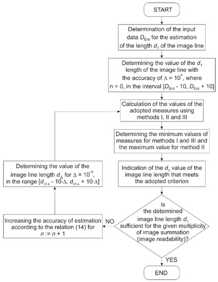
Figure 9. Algorithm of the determining the correct line length $d_{\mathsf{\Delta }}$ of the reconstructed image.

5. Results of Tests and Analyses

5.1. Methods Based on Contrast Assessments

Attempts to estimate the line length based on the image contrast analysis as a function of changes in the length $d_{\mathsf{\Delta }}$ of the line for the given accuracy Δ were carried out based on the dependencies (2), (8), and (11). The analysis was performed with the use of revealing emission signals, the source of which was the primary images presented in Figure 7a,d. The obtained results were visualized in the form of variations of the normalized values of the calculated contrasts as a function of the parameter $d_{\mathsf{\Delta }}$ (Figure 10 and Figure 11). This made it possible to observe the lack of any dependence of contrast on the image line length, and thus prevent the correct estimation of the image line length for the given accuracies.

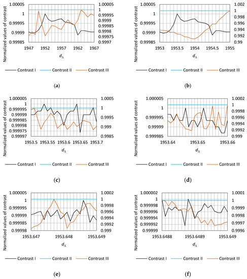
Figure 10. Normalized values of changing of images contrasts calculated according to Equations (2), (8) and (11) in domain of image line length $d_{\mathsf{\Delta }}$ for different accuracies Δ: (a) $\mathsf{\Delta }=1.0$, (b) $\mathsf{\Delta }=0.1$, (c) $\mathsf{\Delta }=0.01$, (d)$\mathsf{\Delta }=0.001$, (e)$\mathsf{\Delta }=0.0001$, (f)$\mathsf{\Delta }=0.00001$, original image Figure 7a.

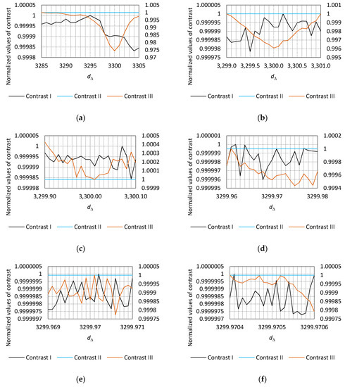
Figure 11. Normalized values of changing of images contrasts calculated according to Equations (2), (8) and (11) in domain of image line length $d_{\mathsf{\Delta }}$ for different accuracies Δ: (a) $\mathsf{\Delta }=1.0$, (b) $\mathsf{\Delta }=0.1$, (c) $\mathsf{\Delta }=0.01$, (d)$\mathsf{\Delta }=0.001$, (e)$\mathsf{\Delta }=0.0001$, (f)$\mathsf{\Delta }=0.00001$, original image Figure 7d.

The changing of the value of the image line length does not affect the quality of the analyzed image. The pixel amplitude values are not modified. Only the number of pixels with given amplitudes changes, which affects the average value of this parameter and the variance of the gray levels of the image ((3), (12)). In the case of the contrast evaluation method described by the dependence (9), the values of $l_{\mathsf{\Delta }\_max}$ and $l_{\mathsf{\Delta }\_max}$ remain constant as a function of changes in $d_{\mathsf{\Delta }}$. Hence, the calculated value of the contrast is constant, making it impossible to estimate the length $d_{\mathsf{\Delta }}$ of the reconstructed image line.

5.2. Proposed Methods of Line Length Estimation of the Reconstructed Image

The analysis to confirm the correctness of the proposed methods and criteria for the estimation of the reconstructed image line length $d_{\mathsf{\Delta }}$ was carried out on the basis of the actual revealing emission signals. Images containing graphic objects of various shapes and qualities, the source of which was the graphic paths of various devices processing protected data, were proposed for the analysis. The obtained results of the analysis show that:

• the proposed methods and criteria meet the requirements for the accuracy of the estimation of image line length $d_{\mathsf{\Delta }}$;
• the accuracy of the estimation of the image line length $d_{\mathsf{\Delta }}$ has an influence on the efficiency of the coherent summation process, the purpose of which is to improve the image quality;
• each of the methods (methods I, II, and III) is effective in the estimation of the image line length $d_{\mathsf{\Delta }}$, regardless of the source of the revealing emission signal and the structure of the data contained in the reconstructed image;
• there may be differences in the estimated values of the image line length $d_{\mathsf{\Delta }}$ depending on the method used. However, this is not a method error. This is due to the fact that the value of the next approximation of the parameter $d_{\mathsf{\Delta }}$ is equal to half the accuracy range. Estimating with an accuracy of Δ one step higher shows that the value $d_{\mathsf{\Delta }}$ is the same regardless of the method used.

It should also be emphasized that in determining the correct length $d_{\mathsf{\Delta }}$ of the image line, the first three stages of estimation are very important, in which the accuracy refers to unity and tenths and hundredths of the line length values after the decimal point. The greater the accuracy (thousandths, ten thousandths, and hundredths of the decimal point), the more difficult it is to visually assess the impact of this accuracy on the quality of the reconstructed image at 30 times, 40 times, or 60 times coherent summation. Therefore, the accuracy of the $d_{\mathsf{\Delta }}$ parameter estimation was limited to the accuracy $\mathsf{\Delta }={10}^{-5}$.

5.2.1. The Source of the Revealing Emission Signal in the Form of a Computer Monitor Working in the HDMI Standard

Figure 7a as a Primary Image, Monitor Mode 1280 × 1024/60 Hz, Pre-Estimated Value $D_{Ent}=1950.00000$

Figure 12, Figure 13, Figure 14, Figure 15, Figure 16 and Figure 17 show the variability of the normalized values of the proposed measures described by the formulas (20, method I), (27, method II), and (30, method III) in the domain of line length $d_{\mathsf{\Delta }}$ of the reconstructed image, examples of reconstructed images for the estimated line lengths $d_{\mathsf{\Delta }}$, for six precision values Δ, and the Table 3, Table 4, Table 5, Table 6, Table 7 and Table 8 include numerical values respectively.

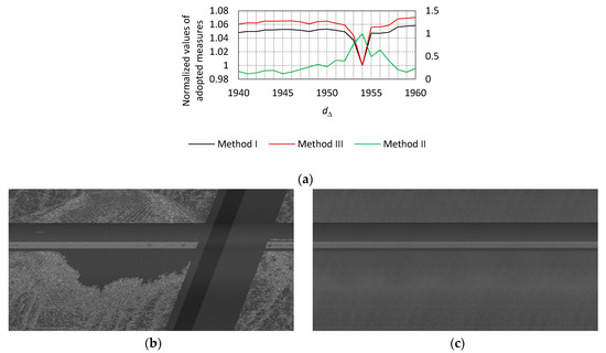
Figure 12. (a) The normalized values of the adopted measures (method I, II and III) calculated in domain of image line length $d_{\mathsf{\Delta }}$ for the accuracy $\mathsf{\Delta }=1.0$ (for the original image shown in Figure 7a) and images reconstructed on the basis of the recorded revealing emission signals at frequency $f_o=1334 \mathrm{MHz}$ (receiving bandwidth $BW=50 \mathrm{MHz}$, accuracy $\mathsf{\Delta }=1.0$), (b) for estimated line length $d_{\mathsf{\Delta }}=1954.00000$, multiple of image summation $Su{m}_{MTL}=1$ and (c) for estimated line length $d_{\mathsf{\Delta }}=1954.00000$, image summation multiple $Su{m}_{MTL}=30$ —the source of revealing signal emission—display monitor, HDMI standard.

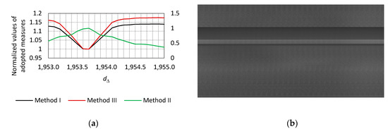
Figure 13. (a) The normalized values of the adopted measures (method I, II and III) calculated in domain of image line length $d_{\mathsf{\Delta }}$ for the accuracy $\mathsf{\Delta }=0.1$ (for the original image shown in Figure 7a) and (b) image reconstructed on the basis of the recorded revealing emission signal at frequency $f_o=1334 \mathrm{MHz}$ (receiving bandwidth $BW=50 \mathrm{MHz}$) for estimated line length $d_{\mathsf{\Delta }}=1953.70000$ (accuracy $\mathsf{\Delta }=0.1$)—multiple of image summation $Su{m}_{MTL}=30$, the source of revealing signal emission—display monitor, HDMI standard.

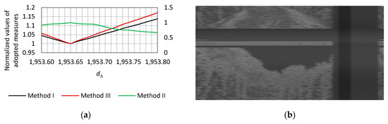
Figure 14. (a) The normalized values of the adopted measures (method I, II and III) calculated in domain of image line length $d_{\mathsf{\Delta }}$ for the accuracy $\mathsf{\Delta }=0.01$ (for the original image shown in Figure 7a) and (b) image reconstructed on the basis of the recorded revealing emission signal at frequency $f_o=1334 \mathrm{MHz}$ (receiving bandwidth $BW=50 \mathrm{MHz}$) for estimated line length $d_{\mathsf{\Delta }}=1953.65000$ (accuracy $\mathsf{\Delta }=0.01$)—multiple of image summation $Su{m}_{MTL}=30$, the source of revealing signal emission—display monitor, HDMI standard.

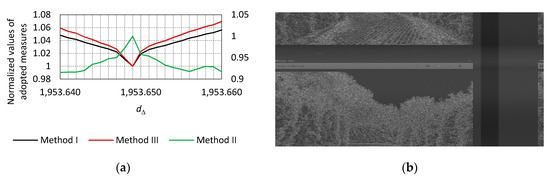
Figure 15. (a) The normalized values of the adopted measures (method I, II and III) calculated in domain of image line length $d_{\mathsf{\Delta }}$ for the accuracy $\mathsf{\Delta }=0.001$ (for the original image shown in Figure 7a) and (b) image reconstructed on the basis of the recorded revealing emission signal at frequency $f_o=1334 \mathrm{MHz}$ (receiving bandwidth $BW=50 \mathrm{MHz}$) for estimated line length $d_{\mathsf{\Delta }}=1953.64900$ (accuracy $\mathsf{\Delta }=0.001$)—multiple of image summation $Su{m}_{MTL}=30$, the source of revealing signal emission—display monitor, HDMI standard.

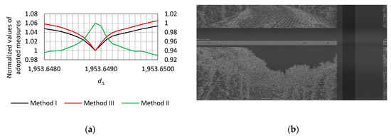
Figure 16. (a) The normalized values of the adopted measures (method I, II and III) calculated in domain of image line length $d_{\mathsf{\Delta }}$ for the accuracy $\mathsf{\Delta }=0.0001$ (for the original image shown in Figure 7a) and (b) image reconstructed on the basis of the recorded revealing emission signal at frequency $f_o=1334 \mathrm{MHz}$ (receiving bandwidth $BW=50 \mathrm{MHz}$) for estimated line length $d_{\mathsf{\Delta }}=1953.64890$ (accuracy $\mathsf{\Delta }=0.0001$)—multiple of image summation $Su{m}_{MTL}=30$, the source of revealing signal emission—display monitor, HDMI standard.

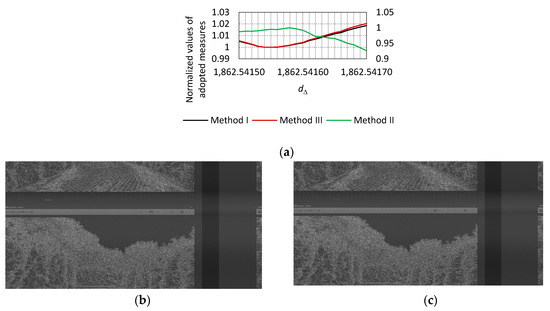
Figure 17. (a) The normalized values of the adopted measures (method I, II and III) calculated in domain of image line length $d_{\mathsf{\Delta }}$ for the accuracy $\mathsf{\Delta }=0.00001$ (for the original image shown in Figure 7a) and images reconstructed on the basis of the recorded revealing emission signals at frequency $f_o=1334 \mathrm{MHz}$ (receiving bandwidth $BW=50 \mathrm{MHz}$, accuracy $\mathsf{\Delta }=0.00001$), (b) for estimated line length $d_{\mathsf{\Delta }}=1953.64892$ and (c) for estimated line length $d_{\mathsf{\Delta }}=1953.64893$ —multiple of image summation $Su{m}_{MTL}=30$, the source of revealing signal emission—display monitor, HDMI standard.

Table 3. Image line length estimation results for the accuracy $\mathsf{\Delta }=1.0$.

Line Length	Method I (Sum of Maxima)	Method II	Method III (Sum of Differences)
1940.00000	1.048164686	0.171849337	1.060336069
1941.00000	1.049776743	0.119365830	1.062373944
1942.00000	1.049735802	0.139908854	1.062203122
1943.00000	1.051995241	0.188569793	1.065041162
1944.00000	1.052210182	0.192791092	1.064795418
1945.00000	1.052829416	0.121851712	1.065092109
1946.00000	1.052688681	0.158177237	1.065244950
1947.00000	1.051619094	0.214366068	1.063806450
1948.00000	1.049786978	0.271374610	1.060929451
1949.00000	1.052517240	0.323367140	1.064339893
1950.00000	1.053200445	0.275619408	1.064837375
1951.00000	1.051567918	0.414920291	1.061684663
1952.00000	1.049485037	0.400918456	1.059254198
1953.00000	1.037366462	0.767506043	1.044102002
1954.00000	1.000000000	1.0000000000	1.000000000
1955.00000	1.047348422	0.493644052	1.056131455
1956.00000	1.047141157	0.644691877	1.056419155
1957.00000	1.048592009	0.401950907	1.058792679
1958.00000	1.056450148	0.212138173	1.068208858
1959.00000	1.057593941	0.155644607	1.069284736
1960.00000	1.058320646	0.238379927	1.070321655

Table 4. Image line length estimation results for the accuracy $\mathsf{\Delta }=0.1$.

Line Length	Method I (Sum of Maxima)	Method II	Method III (Sum of Differences)
1953.00000	1.128509473	0.566120922	1.161644722
1953.10000	1.125077246	0.653023969	1.156506634
1953.20000	1.111804856	0.721004505	1.140902316
1953.30000	1.084614271	0.737559398	1.108103242
1953.40000	1.057994333	0.781928282	1.075430869
1953.50000	1.028688182	0.901126094	1.037330328
1953.60000	1.000887981	0.978394555	1.001363711
1953.70000	1.000000000	1.000000000	1.000000000
1953.80000	1.029002734	0.891301582	1.037963837
1953.90000	1.059216350	0.768574468	1.076867933
1954.00000	1.087859994	0.737611028	1.112577813
1954.10000	1.118237845	0.713704346	1.149291304
1954.20000	1.128598549	0.639065344	1.161598042
1954.30000	1.134547185	0.583418923	1.168143186
1954.40000	1.135833227	0.521527077	1.169590253
1954.50000	1.139154108	0.468060194	1.173558018
1954.60000	1.139677432	0.468250119	1.174621645
1954.70000	1.139666297	0.455018006	1.174571631
1954.80000	1.140390043	0.428413640	1.175481883
1954.90000	1.140484687	0.393074530	1.175985356
1955.00000	1.139368448	0.364117297	1.175028425

Table 5. Image line length estimation results for the accuracy $\mathsf{\Delta }=0.01$.

Line Length	Method I (Sum of Maxima)	Method II	Metoda III (Sum of Differences)
1953.60000	1.045344705	0.918599075	1.057791609
1953.61000	1.035836988	0.941646937	1.046045117
1953.62000	1.025918923	0.958560487	1.033870678
1953.63000	1.017516193	0.961919126	1.022772399
1953.64000	1.008000429	0.975810652	1.010506707
1953.65000	1.000000000	1.000000000	1.000000000
1953.66000	1.011208110	0.967291820	1.014241796
1953.67000	1.019793217	0.955438795	1.025774315
1953.68000	1.027689048	0.951833806	1.035827903
1953.69000	1.037218222	0.949187890	1.047992901
1953.70000	1.046717893	0.906469611	1.059969100
1953.71000	1.056281933	0.857594455	1.071885512
1953.72000	1.064757077	0.809621956	1.082543259
1953.73000	1.073653297	0.781884035	1.093361485
1953.74000	1.084453742	0.757549886	1.107124989
1953.75000	1.092368347	0.751750310	1.117065296
1953.76000	1.101237747	0.730658207	1.127524804
1953.77000	1.109787987	0.709859467	1.138122764
1953.78000	1.119719462	0.694074240	1.149425577
1953.79000	1.128116828	0.683080621	1.159693137
1953.80000	1.137895429	0.663961201	1.171269710

Table 6. Image line length estimation results for the accuracy $\mathsf{\Delta }=0.001$.

Line Length	Method I (Sum of Maxima)	Method II	Method III (Sum of Differences)
1953.64000	1.048187262	0.915623630	1.059534942
1953.64100	1.044262886	0.916235266	1.054277716
1953.64200	1.041631830	0.916434232	1.051271446
1953.64300	1.037312926	0.919930878	1.045627570
1953.64400	1.033866686	0.934525411	1.041464350
1953.64500	1.030198361	0.938919246	1.036374972
1953.64600	1.026825279	0.947507949	1.032361616
1953.64700	1.022394026	0.950160831	1.026633816
1953.64800	1.010795953	0.972321603	1.012636526
1953.64900	1.000000000	1.000000000	1.000000000
1953.65000	1.019321412	0.957806288	1.023055066
1953.65100	1.025816751	0.953613261	1.031168699
1953.65200	1.029516429	0.944418448	1.036000312
1953.65300	1.032178839	0.932808407	1.039597046
1953.65400	1.036202500	0.927301835	1.044560539
1953.65500	1.039350884	0.922611393	1.048876620
1953.65600	1.043601856	0.917858314	1.053747198
1953.65700	1.046295619	0.923716761	1.057322951
1953.65800	1.049843757	0.929676533	1.061552111
1953.65900	1.052396430	0.928444048	1.064444484
1953.66000	1.056344321	0.917217201	1.069629776

Table 7. Image line length estimation results for the accuracy $\mathsf{\Delta }=0.0001$.

Line Length	Method I (Sum of Maxima)	Method II	Method III (Sum of Differences)
1953.64800	1.047916111	0.935641173	1.058259911
1953.64810	1.045866003	0.938583270	1.055964922
1953.64820	1.044235234	0.939182184	1.053807690
1953.64830	1.041377507	0.940372774	1.050721324
1953.64840	1.037893358	0.944932482	1.046389275
1953.64850	1.033995046	0.949683987	1.042033777
1953.64860	1.029035439	0.955727409	1.035925529
1953.64870	1.022455419	0.964475896	1.028451424
1953.64880	1.012168637	0.982063340	1.015938894
1953.64890	1.000000000	1.000000000	1.000000000
1953.64900	1.012631982	0.993629075	1.016237858
1953.64910	1.024290681	0.969259970	1.030444519
1953.64920	1.031554070	0.955114020	1.038885860
1953.64930	1.035268598	0.950946954	1.043698597
1953.64940	1.037782052	0.945884230	1.046538757
1953.64950	1.040688961	0.941543461	1.049927018
1953.64960	1.043665760	0.938248529	1.053394416
1953.64970	1.046683975	0.938706310	1.056685953
1953.64980	1.049039529	0.936455406	1.059701974
1953.64990	1.051485682	0.931872176	1.062794201
1953.65000	1.053745460	0.930100766	1.065200570

Table 8. Image line length estimation results for the accuracy $\mathsf{\Delta }=0.00001$.

Line Length	Method I (Sum of Maxima)	Method II	Method III (Sum of Differences)
1953.64880	1.013086475	0.973197155	1.017277661
1953.64881	1.011788450	0.976878333	1.015880656
1953.64882	1.010249475	0.980919918	1.013835042
1953.64883	1.008472139	0.982972986	1.011472461
1953.64884	1.006959072	0.983571872	1.009685116
1953.64885	1.005168782	0.985128258	1.007539716
1953.64886	1.003829303	0.990618646	1.005705414
1953.64887	1.002909545	0.994455820	1.004408195
1953.64888	1.002176329	0.997080878	1.003193154
1953.64889	1.001256571	0.995492216	1.002098442
1953.64890	1.000906804	0.990971881	1.001317763
1953.64891	1.000652899	0.993801349	1.000845247
1953.64892	1.000000000	0.997548870	1.000000000
1953.64893	1.001266935	1.000000000	1.001473312
1953.64894	1.002689321	0.997882382	1.003193154
1953.64895	1.004210161	0.993274186	1.005259312
1953.64896	1.006352809	0.987575802	1.008114954
1953.64897	1.008254506	0.989293565	1.010662433
1953.64898	1.010296110	0.989584043	1.013295023
1953.64899	1.011969811	0.988384478	1.015352377
1953.64900	1.013550241	0.984658474	1.017577019

Table 9 shows the estimated values of the line length $d_{\mathsf{\Delta }}$ of the analyzed image. These are the values for which the criteria of the adopted methods have been met, allowing to carry out the process of estimating the image line length for the next accuracy step Δ.

Table 9. Estimated lines lengths $d_{\mathsf{\Delta }}$ of the reconstructed image for a given accuracy Δ using the methods proposed by the authors.

Accuracy	Method I $\mathit{S}\mathit{u}\mathit{m}\_\mathit{m}\mathit{i}{\mathit{n}}_{\mathit{M}\mathit{e}\mathit{t}\_\mathit{I}\_\mathit{U}\mathit{n}}\left(\mathsf{\Delta }\right)$	Method II $\mathit{D}\mathit{i}\mathit{f}\_\mathit{m}\mathit{a}{\mathit{x}}_{\mathit{M}\mathit{e}\mathit{t}\_\mathit{I}\mathit{I}\_\mathit{U}\mathit{n}}\left(\mathsf{\Delta }\right)$	Method III $\mathit{S}\mathit{u}\mathit{m}\_\mathit{m}\mathit{i}{\mathit{n}}_{\mathit{M}\mathit{e}\mathit{t}\_\mathit{I}\mathit{I}\mathit{I}\_\mathit{U}\mathit{n}}\left(\mathsf{\Delta }\right)$
$\mathsf{\Delta }=1.0$	1954.00000	1954.00000	1954.00000
$\mathsf{\Delta }=0.1$	1953.70000	1953.70000	1953.70000
$\mathsf{\Delta }=0.01$	1953.65000	1953.65000	1953.65000
$\mathsf{\Delta }=0.001$	1953.64900	1953.64900	1953.64900
$\mathsf{\Delta }=0.0001$	1953.64890	1953.64890	1953.64890
$\mathsf{\Delta }=0.00001$	1953.64892	1953.64893	1953.64892

Figure 7b as a Primary Image, Monitor Mode 1280 × 1024/60 Hz, Pre-Estimated Value $D_{Ent}=1957.00000$

Figure 18, Figure 19 and Figure 20 show the variability of the normalized values of the proposed measures described by the formulas (20, method I), (27, method II) and (30, method III) in domain of the line length $d_{\mathsf{\Delta }}$ of the reconstructed image, examples of reconstructed images for the estimated line length $d_{\mathsf{\Delta }}$, for six precision values Δ.

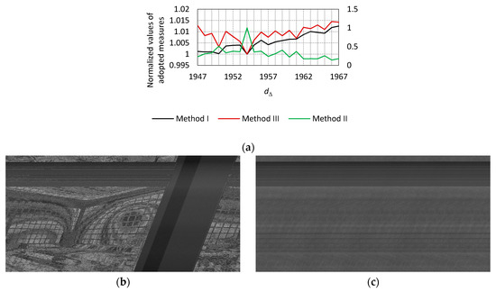
Figure 18. (a) The normalized values of the adopted measures (method I, II and III) calculated in domain of image line length $d_{\mathsf{\Delta }}$ for the accuracy $\mathsf{\Delta }=1.0$ (for the original image shown in Figure 7b) and images reconstructed on the basis of the recorded revealing emission signals at frequency $f_o=1334 \mathrm{MHz}$ (receiving bandwidth $BW=50 \mathrm{MHz}$, accuracy $\mathsf{\Delta }=1.0$), (b) for estimated line length $d_{\mathsf{\Delta }}=1954.00000$, multiple of image summation $Su{m}_{MTL}=1$ and (c) for estimated line length $d_{\mathsf{\Delta }}=1954.00000$, image summation multiple $Su{m}_{MTL}=30$ —the source of revealing signal emission—display monitor, HDMI standard.

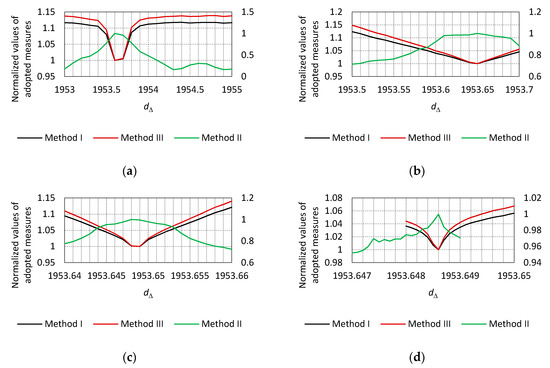
Figure 19. The normalized values of the adopted measures (method I, II and III) calculated in domain of image line length $d_{\mathsf{\Delta }}$ for the accuracy (a) $\mathsf{\Delta }=0.1$, (b) $\mathsf{\Delta }=0.01$, (c) $\mathsf{\Delta }=0.001$ and (d) $\mathsf{\Delta }=0.0001$ (for the original image shown in Figure 7b).

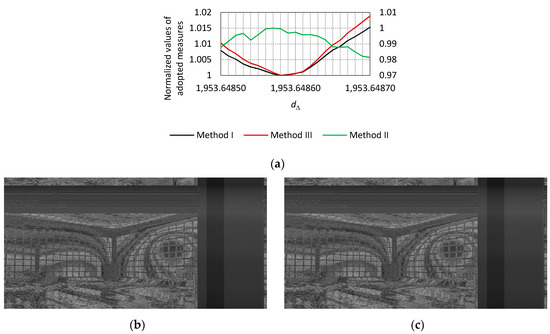
Figure 20. (a) The normalized values of the adopted measures (method I, II and III) calculated in domain of image line length $d_{\mathsf{\Delta }}$ for the accuracy $\mathsf{\Delta }=0.00001$ (for the original image shown in Figure 7b) and images reconstructed on the basis of the recorded revealing emission signals at frequency $f_o=1334 \mathrm{MHz}$ (receiving bandwidth $BW=50 \mathrm{MHz}$, accuracy $\mathsf{\Delta }=0.00001$), (b) for estimated line length $d_{\mathsf{\Delta }}=1953.64857$ and (c) for estimated line length $d_{\mathsf{\Delta }}=1953.64858$ —multiple of image summation $Su{m}_{MTL}=30$, the source of revealing signal emission—display monitor, HDMI standard.

Table 10 shows the estimated values of the line length $d_{\mathsf{\Delta }}$ of the analyzed image. These are the values for which the criteria of the adopted methods have been met, allowing us to carry out the process of estimating the image line length for the next accuracy step Δ.

Table 10. Estimated lines lengths $d_{\mathsf{\Delta }}$ of the reconstructed image for a given accuracy Δ using the methods proposed by the authors.

Accuracy	Method I $\mathit{S}\mathit{u}\mathit{m}\_\mathit{m}\mathit{i}{\mathit{n}}_{\mathit{M}\mathit{e}\mathit{t}\_\mathit{I}\_\mathit{U}\mathit{n}}\left(\mathsf{\Delta }\right)$	Method II $\mathit{D}\mathit{i}\mathit{f}\_\mathit{m}\mathit{a}{\mathit{x}}_{\mathit{M}\mathit{e}\mathit{t}\_\mathit{I}\mathit{I}\_\mathit{U}\mathit{n}}\left(\mathsf{\Delta }\right)$	Method III $\mathit{S}\mathit{u}\mathit{m}\_\mathit{m}\mathit{i}{\mathit{n}}_{\mathit{M}\mathit{e}\mathit{t}\_\mathit{I}\mathit{I}\mathit{I}\_\mathit{U}\mathit{n}}\left(\mathsf{\Delta }\right)$
$\mathsf{\Delta }=1.0$	1954.00000	1954.00000	1954.00000
$\mathsf{\Delta }=0.1$	1953.60000	1953.60000	1953.60000
$\mathsf{\Delta }=0.01$	1953.65000	1953.65000	1953.65000
$\mathsf{\Delta }=0.001$	1953.64800	1953.64800	1953.64900
$\mathsf{\Delta }=0.0001$	1953.64860	1953.64860	1953.64860
$\mathsf{\Delta }=0.00001$	1953.64858	1953.64857	1953.64858

Figure 7c as a Primary Image, Monitor Mode 1280 × 1024/60 Hz, Pre-Estimated Value $D_{Ent}=3904.00000$

Figure 21, Figure 22 and Figure 23 show the variability of the normalized values of the proposed measures described by the dependencies (20, method I), (27, method II), and (30, method III) in the domain of line length $d_{\mathsf{\Delta }}$ of the reconstructed image, examples of reconstructed images for the estimated line length $d_{\mathsf{\Delta }}$, for six precision values Δ.

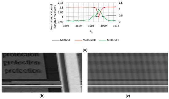
Figure 21. (a) The normalized values of the adopted measures (method I, II and III) calculated in domain of image line length $d_{\mathsf{\Delta }}$ for the accuracy $\mathsf{\Delta }=1.0$ (for the original image shown in Figure 7c) and images reconstructed on the basis of the recorded revealing emission signals at frequency $f_o=768 \mathrm{MHz}$ (receiving bandwidth $BW=50 \mathrm{MHz}$, accuracy $\mathsf{\Delta }=1.0$), (b) for estimated line length $d_{\mathsf{\Delta }}=3907.00000$, image summation multiple $Su{m}_{MTL}=1$ and (c) for estimated line length $d_{\mathsf{\Delta }}=3907.00000$, multiple of image summation $Su{m}_{MTL}=60$ —the source of revealing signal emission—display monitor, HDMI standard.

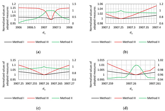
Figure 22. The normalized values of the adopted measures (method I, II and III) calculated in domain of image line length $d_{\mathsf{\Delta }}$ for the accuracy (a) $\mathsf{\Delta }=0.1$, (b) $\mathsf{\Delta }=0.01$, (c) $\mathsf{\Delta }=0.001$ and (d) $\mathsf{\Delta }=0.0001$ (for the original image shown in Figure 7c).

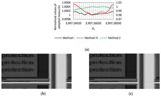
Figure 23. (a) The normalized values of the adopted measures (method I, II and III) calculated in domain of image line length $d_{\mathsf{\Delta }}$ for the accuracy $\mathsf{\Delta }=0.00001$ (for the original image shown in Figure 7c) and images reconstructed on the basis of the recorded revealing emission signals at frequency $f_o=768 \mathrm{MHz}$ (receiving bandwidth $BW=50 \mathrm{MHz}$, accuracy $\mathsf{\Delta }=0.00001$), (b) for estimated line length $d_{\mathsf{\Delta }}=3907.26019$ and (c) for estimated line length $d_{\mathsf{\Delta }}=3907.26025$ —multiple of image summation $Su{m}_{MTL}=60$, the source of revealing signal emission—display monitor, HDMI standard.

Table 11 shows the estimated values of the line length $d_{\mathsf{\Delta }}$ of the analyzed image. These are the values for which the criteria of the adopted methods have been met, allowing us to carry out the process of estimating the image line length for the next accuracy step Δ.

Table 11. Estimated lines lengths $d_{\mathsf{\Delta }}$ of the reconstructed image for a given accuracy Δ using the methods proposed by the authors.

Accuracy	Method I $\mathit{S}\mathit{u}\mathit{m}\_\mathit{m}\mathit{i}{\mathit{n}}_{\mathit{M}\mathit{e}\mathit{t}\_\mathit{I}\_\mathit{U}\mathit{n}}\left(\mathsf{\Delta }\right)$	Method II $\mathit{D}\mathit{i}\mathit{f}\_\mathit{m}\mathit{a}{\mathit{x}}_{\mathit{M}\mathit{e}\mathit{t}\_\mathit{I}\mathit{I}\_\mathit{U}\mathit{n}}\left(\mathsf{\Delta }\right)$	Method III $\mathit{S}\mathit{u}\mathit{m}\_\mathit{m}\mathit{i}{\mathit{n}}_{\mathit{M}\mathit{e}\mathit{t}\_\mathit{I}\mathit{I}\mathit{I}\_\mathit{U}\mathit{n}}\left(\mathsf{\Delta }\right)$
$\mathsf{\Delta }=1.0$	3907.00000	3907.00000	3907.00000
$\mathsf{\Delta }=0.1$	3907.30000	3907.30000	3907.30000
$\mathsf{\Delta }=0.01$	3907.26000	3907.26000	3907.26000
$\mathsf{\Delta }=0.001$	3907.26000	3907.26000	3907.26000
$\mathsf{\Delta }=0.0001$	3907.26020	3907.26020	3907.26020
$\mathsf{\Delta }=0.00001$	3907.26019	3907.26025	3907.26019

5.2.2. The Source of the Revealing Emission Signal in the Form of a Computer Monitor Working in the VGA Standard

Figure 7d as a Primary Image, Monitor Mode 1280 × 1024/60 Hz, Pre-Estimated Value $D_{\mathrm{Ent}}=3295.00000$

Figure 24, Figure 25, Figure 26, Figure 27, Figure 28 and Figure 29 show the variability of the normalized values of the proposed measures described by the formulas (20, method I), (27, method II), and (30, method III) in the domain of the line length $d_{\mathsf{\Delta }}$ of the reconstructed image, examples of reconstructed images for the estimated line length $d_{\mathsf{\Delta }}$, for six precision values Δ, and the Table 12, Table 13, Table 14, Table 15, Table 16 and Table 17 include numerical values respectively.

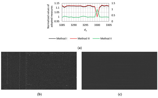
Figure 24. (a) The normalized values of the adopted measures (method I, II and III) calculated in domain of image line length $d_{\mathsf{\Delta }}$ for the accuracy $\mathsf{\Delta }=1.0$ (for the original image shown in Figure 7d) and images reconstructed on the basis of the recorded revealing emission signals at frequency $f_o=740 \mathrm{MHz}$ (receiving bandwidth $BW=50 \mathrm{MHz}$, accuracy $\mathsf{\Delta }=1.0$), (b) for estimated line length $d_{\mathsf{\Delta }}=3300.00000$, image summation multiple $Su{m}_{MTL}=1$ and (c) for estimated line length $d_{\mathsf{\Delta }}=3300.00000$, multiple of image summation $Su{m}_{MTL}=60$ —the source of revealing signal emission—display monitor, VGA standard.

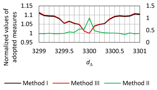
Figure 25. The normalized values of the adopted measures (method I, II and III) calculated in domain of image line length $d_{\mathsf{\Delta }}$ for the accuracy $\mathsf{\Delta }=0.1$ (for the original image shown in Figure 7d).

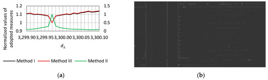
Figure 26. (a) The normalized values of the adopted measures (method I, II and III) calculated in domain of image line length $d_{\mathsf{\Delta }}$ for the accuracy $\mathsf{\Delta }=0.01$ (for the original image shown in Figure 7d) and (b) image reconstructed on the basis of the recorded revealing emission signal at frequency $f_o=740 \mathrm{MHz}$ (receiving bandwidth $BW=50 \mathrm{MHz}$) for estimated line length $d_{\mathsf{\Delta }}=3299.97000$ (accuracy $\mathsf{\Delta }=0.01$)—multiple of image summation $Su{m}_{MTL}=60$, the source of revealing signal emission—display monitor, VGA standard.

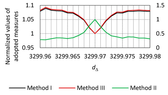
Figure 27. The normalized values of the adopted measures (method I, II and III) calculated in domain of image line length $d_{\mathsf{\Delta }}$ for the accuracy $\mathsf{\Delta }=0.001$ (for the original image shown in Figure 7d).

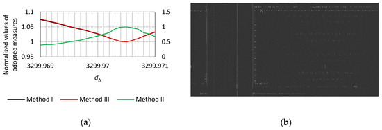
Figure 28. (a) The normalized values of the adopted measures (method I, II and III) calculated in domain of image line length $d_{\mathsf{\Delta }}$ for the accuracy $\mathsf{\Delta }=0.0001$ (for the original image shown in Figure 7d) and (b) image reconstructed on the basis of the recorded revealing emission signal at frequency $f_o=740 \mathrm{MHz}$ (receiving bandwidth $BW=50 \mathrm{MHz}$) for estimated line length $d_{\mathsf{\Delta }}=3299.97050$ (accuracy $\mathsf{\Delta }=0.0001$)—multiple of image summation $Su{m}_{MTL}=60$, the source of revealing signal emission—display monitor, VGA standard.

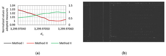
Figure 29. (a) The normalized values of the adopted measures (method I, II and III) calculated in domain of image line length $d_{\mathsf{\Delta }}$ for the accuracy $\mathsf{\Delta }=0.00001$ (for the original image shown in Figure 7d) and (b) image reconstructed on the basis of the recorded revealing emission signal at frequency $f_o=740 \mathrm{MHz}$ (receiving bandwidth $BW=50 \mathrm{MHz}$) for estimated line length $d_{\mathsf{\Delta }}=3299.97057$ (accuracy $\mathsf{\Delta }=0.00001$)—multiple of image summation $Su{m}_{MTL}=60$, the source of revealing signal emission—display monitor, VGA standard.

Table 12. Image line length estimation results for the accuracy $\mathsf{\Delta }=1.0$.

Line Length	Method I (Sum of Maxima)	Method II	Method III (Sum of Differences)
3285.00000	1.120522806	0.323730914	1.125336744
3286.00000	1.104016613	0.432052882	1.107925178
3287.00000	1.117467594	0.390075927	1.122010671
3288.00000	1.119587273	0.337887334	1.124127670
3289.00000	1.118140143	0.369545949	1.122608500
3290.00000	1.118529589	0.310561218	1.122985683
3291.00000	1.116974679	0.343311144	1.121372590
3292.00000	1.117172995	0.317745072	1.121700576
3293.00000	1.118140143	0.382540274	1.122656207
3294.00000	1.110786652	0.432827259	1.114915745
3295.00000	1.111799787	0.400781984	1.116100966
3296.00000	1.121648033	0.339014565	1.126334119
3297.00000	1.122117955	0.364968354	1.126641233
3298.00000	1.111444831	0.350635507	1.115793852
3299.00000	1.110217573	0.359650189	1.114538561
3300.00000	1.000000000	1.000000000	1.000000000
3301.00000	1.102570919	0.368348992	1.106411971
3302.00000	1.125029460	0.346655863	1.129843566
3303.00000	1.117453223	0.357396782	1.121740829
3304.00000	1.122641048	0.365919158	1.127259933
3305.00000	1.116596729	0.335950862	1.120998388

Table 13. Image line length estimation results for the accuracy $\mathsf{\Delta }=0.1$.

Line Length	Method I (Sum of Maxima)	Method II	Method III (Sum of Differences)
3299.00000	1.1102176	0.3596502	1.11453856
3299.10000	1.0960179	0.3559526	1.09968081
3299.20000	1.0931351	0.3773985	1.09668720
3299.30000	1.0919308	0.3524315	1.09542445
3299.40000	1.0796080	0.3579599	1.08254654
3299.50000	1.0537335	0.3713768	1.05579633
3299.60000	1.0645288	0.4302210	1.06709096
3299.70000	1.0535481	0.4144102	1.05553990
3299.80000	1.0476346	0.5481207	1.04929028
3299.90000	1.0113615	0.5532276	1.01169120
3300.00000	1.0000000	1.0000000	1.00000000
3300.10000	1.0389130	0.4809306	1.04041529
3300.20000	1.0481117	0.4251500	1.04971965
3300.30000	1.0519056	0.3952525	1.05394470
3300.40000	1.0758242	0.3835967	1.07886117
3300.50000	1.0900095	0.3816243	1.09338349
3300.60000	1.0937861	0.3704260	1.09732379
3300.70000	1.0913503	0.3250346	1.09486240
3300.80000	1.0933579	0.3877169	1.09676323
3300.90000	1.1046935	0.3532766	1.10863184
3301.00000	1.1025709	0.368349	1.10641197

Table 14. Image line length estimation results for the accuracy $\mathsf{\Delta }=0.01$.

Line Length	Method I (Sum of Maxima)	Method II	Method III (Sum of Differences)
3299.90000	1.1065329	0.1001021	1.11093412
3299.91000	1.1101728	0.1067478	1.11472726
3299.92000	1.0972044	0.1267683	1.10126874
3299.93000	1.0987343	0.1526061	1.10293858
3299.94000	1.0948727	0.2019888	1.09886386
3299.95000	1.0880725	0.2282842	1.09176380
3299.96000	1.0790475	0.2859177	1.08244385
3299.97000	1.0000000	1.0000000	1.00000000
3299.98000	1.0787582	0.3141782	1.08193471
3299.99000	1.0863917	0.2101435	1.09024131
3300.00000	1.0941023	0.1809419	1.09809606
3300.01000	1.1011415	0.1464637	1.10543350
3300.02000	1.0960991	0.1220722	1.10017353
3300.03000	1.1125737	0.1139609	1.11731877
3300.04000	1.1058521	0.1041928	1.11026128
3300.05000	1.1185217	0.1026445	1.12353644
3300.06000	1.1233377	0.1029948	1.12852465
3300.07000	1.1337793	0.0828789	1.13951116
3300.08000	1.1249540	0.0874667	1.13018303
3300.09000	1.1293297	0.0897860	1.13480126
3300.10000	1.1366771	0.0870205	1.14247593

Table 15. Image line length estimation results for the accuracy $\mathsf{\Delta }=0.001$.

Line Length	Method I (Sum of Maxima)	Method II	Method III (Sum of Differences)
3299.96000	1.0790475	0.2859177	1.08244385
3299.96100	1.0893115	0.2828917	1.09298834
3299.96200	1.0826559	0.3178542	1.08592266
3299.96300	1.0807959	0.3525624	1.08415788
3299.96400	1.0798509	0.3469921	1.08322147
3299.96500	1.0731183	0.3249460	1.07620654
3299.96600	1.0723102	0.3557852	1.07523902
3299.96700	1.0613827	0.4351092	1.06394637
3299.96800	1.0473719	0.5440873	1.04917491
3299.96900	1.0199148	0.7887994	1.02091219
3299.97000	1.0000000	1.0000000	1.00000000
3299.97100	1.0194950	0.7488153	1.02055039
3299.97200	1.0448578	0.5460046	1.04697629
3299.97300	1.0621484	0.4208681	1.06468142
3299.97400	1.0734092	0.3855616	1.07646356
3299.97500	1.0727976	0.3406400	1.07588403
3299.97600	1.0787566	0.3861485	1.08197400
3299.97700	1.0790318	0.3797313	1.08228669
3299.97800	1.0802943	0.3412574	1.08381409
3299.97900	1.0792503	0.3434442	1.08242420
3299.98000	1.0787582	0.3141782	1.08193471

Table 16. Image line length estimation results for the accuracy $\mathsf{\Delta }=0.0001$.

Line Length	Method I (Sum of Maxima)	Method II	Method III (Sum of Differences)
3299.96900	1.0744817	0.3952254	1.07634270
3299.96910	1.0698641	0.4139846	1.07162301
3299.96920	1.0657144	0.4152352	1.06723052
3299.96930	1.0612688	0.4380820	1.06257508
3299.96940	1.0563131	0.4652010	1.05762680
3299.96950	1.0508035	0.4998636	1.05176865
3299.96960	1.0466946	0.5284766	1.04755096
3299.96970	1.0419517	0.5556020	1.04288506
3299.96980	1.0375221	0.6056936	1.03830581
3299.96990	1.0314907	0.6494630	1.03220413
3299.97000	1.0266283	0.6950076	1.02732160
3299.97010	1.0201611	0.7520679	1.02062379
3299.97020	1.0129796	0.8095374	1.01314162
3299.97030	1.0066961	0.9292102	1.00685767
3299.97040	1.0016150	0.9895628	1.00166138
3299.97050	1.0000000	1.0000000	1.00000000
3299.97060	1.0044368	0.9686088	1.00431331
3299.97070	1.0110148	0.9258592	1.01114856
3299.97080	1.0186860	0.8031710	1.01899678
3299.97090	1.0257275	0.7638585	1.02624140
3299.97100	1.0324483	0.6732079	1.03321411

Table 17. Image line length estimation results for the accuracy $\mathsf{\Delta }=0.00001$.

Line Length	Method I (Sum of Maxima)	Method II	Method III (Sum of Differences)
3299.97040	1.0284502	0.5531938	1.02893843
3299.97041	1.0270844	0.5702378	1.02746142
3299.97042	1.0256717	0.5866089	1.02607795
3299.97043	1.0235286	0.6073334	1.02392526
3299.97044	1.0210823	0.6294182	1.02157992
3299.97045	1.0201479	0.6575501	1.02059153
3299.97046	1.0178256	0.6879719	1.01818755
3299.97047	1.0157749	0.7274403	1.01615493
3299.97048	1.0140921	0.7677313	1.01441128
3299.97049	1.0112378	0.8123110	1.01150752
3299.97050	1.0090989	0.8526606	1.00931994
3299.97051	1.0079936	0.8862900	1.00824359
3299.97052	1.0048416	0.9016767	1.00508715
3299.97053	1.0014099	0.8954113	1.00154960
3299.97054	1.0012321	0.944773	1.00135974
3299.97055	1.0007001	0.9693599	1.00079714
3299.97056	1.0000165	0.9993997	1.00006841
3299.97057	1.0000000	1.0000000	1.00000000
3299.97058	1.0005885	0.9666031	1.00065195
3299.97059	1.0024890	0.9549048	1.00262594
3299.97060	1.0038328	0.9534355	1.00399825

Table 18 shows the estimated values of the line length $d_{\mathsf{\Delta }}$ of the analyzed image. These are the values for which the criteria of the adopted methods have been met, allowing us to carry out the process of estimating the image line length for the next accuracy step Δ.

Table 18. Estimated lines lengths $d_{\mathsf{\Delta }}$ of the reconstructed image for a given accuracy Δ using the methods proposed by the authors.

Accuracy	Method I $\mathit{S}\mathit{u}\mathit{m}\_\mathit{m}\mathit{i}{\mathit{n}}_{\mathit{M}\mathit{e}\mathit{t}\_\mathit{I}\_\mathit{U}\mathit{n}}\left(\mathsf{\Delta }\right)$	Method II $\mathit{D}\mathit{i}\mathit{f}\_\mathit{m}\mathit{a}{\mathit{x}}_{\mathit{M}\mathit{e}\mathit{t}\_\mathit{I}\mathit{I}\_\mathit{U}\mathit{n}}\left(\mathsf{\Delta }\right)$	Method III $\mathit{S}\mathit{u}\mathit{m}\_\mathit{m}\mathit{i}{\mathit{n}}_{\mathit{M}\mathit{e}\mathit{t}\_\mathit{I}\mathit{I}\mathit{I}\_\mathit{U}\mathit{n}}\left(\mathsf{\Delta }\right)$
$\mathsf{\Delta }=1.0$	3300.00000	3300.00000	3300.00000
$\mathsf{\Delta }=0.1$	3300.00000	3300.00000	3300.00000
$\mathsf{\Delta }=0.01$	3299.97000	3299.97000	3299.97000
$\mathsf{\Delta }=0.001$	3299.97000	3299.97000	3299.97000
$\mathsf{\Delta }=0.0001$	3299.97050	3299.97050	3299.97050
$\mathsf{\Delta }=0.00001$	3299.97057	3299.97057	3299.97057

Figure 7e as a Primary Image, Monitor Mode 1280 × 1024/60 Hz, Pre-Estimated Value $D_{Ent}=3310.00000$

Figure 30, Figure 31 and Figure 32 show the variability of the normalized values of the proposed measures described by the formulas (20, method I), (27, method II), and (30, method III) in the domain of the line length $d_{\mathsf{\Delta }}$ of the reconstructed image, examples of reconstructed images for the estimated line length $d_{\mathsf{\Delta }}$, for six precision values Δ.

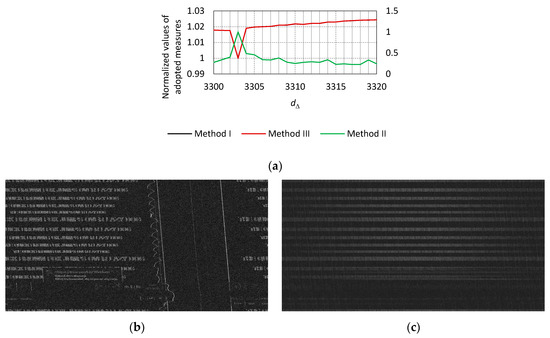
Figure 30. (a) The normalized values of the adopted measures (method I, II and III) calculated in domain of image line length $d_{\mathsf{\Delta }}$ for the accuracy $\mathsf{\Delta }=1.0$ (for the original image shown in Figure 7e) and images reconstructed on the basis of the recorded revealing emission signals at frequency $f_o=450 \mathrm{MHz}$ (receiving bandwidth $BW=50 \mathrm{MHz}$, accuracy $\mathsf{\Delta }=1.0$), (b) for estimated line length $d_{\mathsf{\Delta }}=3303.00000$, image summation multiple $Su{m}_{MTL}=1$ and (c) for estimated line length $d_{\mathsf{\Delta }}=3300.00000$, multiple of image summation $Su{m}_{MTL}=15$ —the source of revealing signal emission—display monitor, VGA standard.

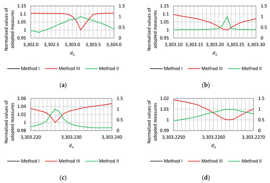
Figure 31. The normalized values of the adopted measures (method I, II and III) calculated in domain of image line length $d_{\mathsf{\Delta }}$ for the accuracy (a) $\mathsf{\Delta }=0.1$, (b) $\mathsf{\Delta }=0.01$, (c) $\mathsf{\Delta }=0.001$ and (d) $\mathsf{\Delta }=0.0001$ (for the original image shown in Figure 7e).

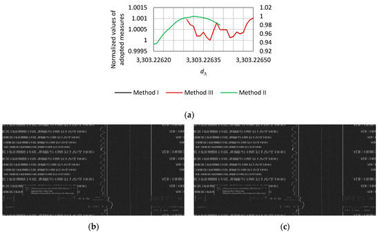
Figure 32. (a) The normalized values of the adopted measures (method I, II and III) calculated in domain of image line length $d_{\mathsf{\Delta }}$ for the accuracy $\mathsf{\Delta }=0.00001$ (for the original image shown in Figure 7e) and images reconstructed on the basis of the recorded revealing emission signals at frequency $f_o=450 \mathrm{MHz}$ (receiving bandwidth $BW=50 \mathrm{MHz}$, accuracy $\mathsf{\Delta }=0.00001$), (b) for estimated line length $d_{\mathsf{\Delta }}=3303.22632$ and (c) for estimated line length $d_{\mathsf{\Delta }}=3303.22637$ —multiple of image summation $Su{m}_{MTL}=15$, the source of revealing signal emission—display monitor, VGA standard.

Table 19 shows the estimated values of the line length $d_{\mathsf{\Delta }}$ of the analyzed image. These are the values for which the criteria of the adopted methods have been met, allowing us to carry out the process of estimating the image line length for the next accuracy step Δ.

Table 19. Estimated lines lengths $d_{\mathsf{\Delta }}$ of the reconstructed image for a given accuracy Δ using the methods proposed by the authors.

Accuracy	Method I $\mathit{S}\mathit{u}\mathit{m}\_\mathit{m}\mathit{i}{\mathit{n}}_{\mathit{M}\mathit{e}\mathit{t}\_\mathit{I}\_\mathit{U}\mathit{n}}\left(\mathsf{\Delta }\right)$	Method II $\mathit{D}\mathit{i}\mathit{f}\_\mathit{m}\mathit{a}{\mathit{x}}_{\mathit{M}\mathit{e}\mathit{t}\_\mathit{I}\mathit{I}\_\mathit{U}\mathit{n}}\left(\mathsf{\Delta }\right)$	Method III $\mathit{S}\mathit{u}\mathit{m}\_\mathit{m}\mathit{i}{\mathit{n}}_{\mathit{M}\mathit{e}\mathit{t}\_\mathit{I}\mathit{I}\mathit{I}\_\mathit{U}\mathit{n}}\left(\mathsf{\Delta }\right)$
$\mathsf{\Delta }=1.0$	3303.00000	3303.00000	3303.00000
$\mathsf{\Delta }=0.1$	3303.20000	3303.20000	3303.20000
$\mathsf{\Delta }=0.01$	3303.23000	3303.23000	3303.23000
$\mathsf{\Delta }=0.001$	3303.22600	3303.22600	3303.22600
$\mathsf{\Delta }=0.0001$	3303.22640	3303.22630	3303.22640
$\mathsf{\Delta }=0.00001$	3303.22637	3303.22632	3303.22637

5.2.3. The Source of the Revealing Emission Signal in the Form of Display of Laser Printer

Figure 7f as a Primary Image, Display Mode Unknown, Pre-Estimated Value $D_{Ent}=1857.00000$

Figure 33, Figure 34 and Figure 35 show the variability of the normalized values of the proposed measures described by the formulas (20, method I), (27, method II), and (30, method III) in the domain of the line length $d_{\mathsf{\Delta }}$ of the reconstructed image, examples of reconstructed images for the estimated line length $d_{\mathsf{\Delta }}$, for six precision values Δ.

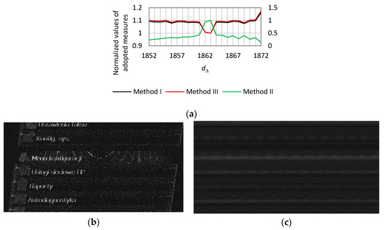
Figure 33. (a) The normalized values of the adopted measures (method I, II and III) calculated in domain of image line length $d_{\mathsf{\Delta }}$ for the accuracy $\mathsf{\Delta }=1.0$ (for the original image shown in Figure 7f) and images reconstructed on the basis of the recorded revealing emission signals at frequency $f_o=235 \mathrm{MHz}$ (receiving bandwidth $BW=10 \mathrm{MHz}$, accuracy $\mathsf{\Delta }=1.0$), (b) for estimated line length $d_{\mathsf{\Delta }}=1863.00000$, image summation multiple $Su{m}_{MTL}=1$ and (c) for estimated line length $d_{\mathsf{\Delta }}=1863.00000$, multiple of image summation $Su{m}_{MTL}=60$ —the source of revealing signal emission—display of laser printer.

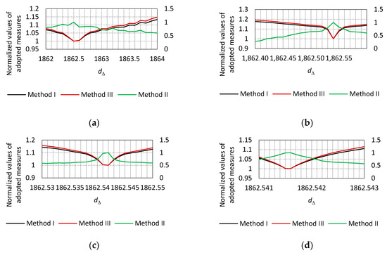
Figure 34. The normalized values of the adopted measures (method I, II and III) calculated in domain of image line length $d_{\mathsf{\Delta }}$ for the accuracy (a) $\mathsf{\Delta }=0.1$, (b) $\mathsf{\Delta }=0.01$, (c) $\mathsf{\Delta }=0.001$ and (d) $\mathsf{\Delta }=0.0001$ (for the original image shown in Figure 7f).

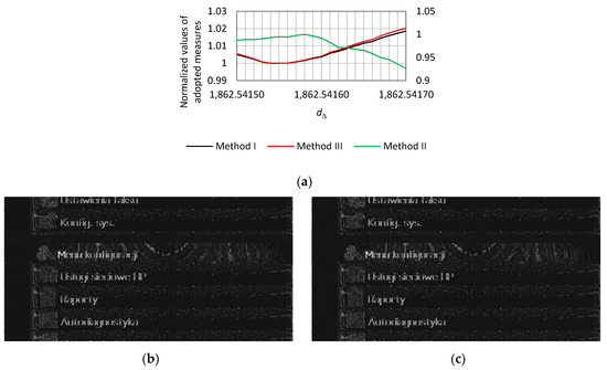
Figure 35. (a) The normalized values of the adopted measures (method I, II and III) calculated in domain of image line length $d_{\mathsf{\Delta }}$ for the accuracy $\mathsf{\Delta }=0.00001$ (for the original image shown in Figure 7f) and images reconstructed on the basis of the recorded revealing emission signals at frequency $f_o=235 \mathrm{MHz}$ (receiving bandwidth $BW=10 \mathrm{MHz}$, accuracy $\mathsf{\Delta }=0.00001$), (b) for estimated line length $d_{\mathsf{\Delta }}=1862.54155$ and (c) for estimated line length $d_{\mathsf{\Delta }}=1862.54158$ —multiple of image summation $Su{m}_{MTL}=15$, the source of revealing signal emission—display of laser printer.

Table 20 shows the estimated values of the line length $d_{\mathsf{\Delta }}$ of the analyzed image. These are the values for which the criteria of the adopted methods have been met, allowing us to carry out the process of estimating the image line length for the next accuracy step Δ.

Table 20. Estimated lines lengths $d_{\mathsf{\Delta }}$ of the reconstructed image for a given accuracy Δ using the methods proposed by the authors.

Accuracy	Method I $\mathit{S}\mathit{u}\mathit{m}\_\mathit{m}\mathit{i}{\mathit{n}}_{\mathit{M}\mathit{e}\mathit{t}\_\mathit{I}\_\mathit{U}\mathit{n}}\left(\mathsf{\Delta }\right)$	Method II $\mathit{D}\mathit{i}\mathit{f}\_\mathit{m}\mathit{a}{\mathit{x}}_{\mathit{M}\mathit{e}\mathit{t}\_\mathit{I}\mathit{I}\_\mathit{U}\mathit{n}}\left(\mathsf{\Delta }\right)$	Method III $\mathit{S}\mathit{u}\mathit{m}\_\mathit{m}\mathit{i}{\mathit{n}}_{\mathit{M}\mathit{e}\mathit{t}\_\mathit{I}\mathit{I}\mathit{I}\_\mathit{U}\mathit{n}}\left(\mathsf{\Delta }\right)$
$\mathsf{\Delta }=1.0$	1863.00000	1863.00000	1863.00000
$\mathsf{\Delta }=0.1$	1862.50000	1862.50000	1862.50000
$\mathsf{\Delta }=0.01$	1862.54000	1862.54000	1862.54000
$\mathsf{\Delta }=0.001$	1862.54200	1862.54200	1862.54200
$\mathsf{\Delta }=0.0001$	1862.54160	1862.54160	1862.54160
$\mathsf{\Delta }=0.00001$	1862.54155	1862.54158	1862.54155

6. Conclusions from the Analysis, Recommendations for the Software Implementation of Automatic Image Recognition

The article presents the issue related to the correct determination of the line length of the reconstructed image on the basis of the recorded revealing emission signal. The correct line length ensures that the graphic elements contained in the image remain vertical. They are not tilted to the left or right. Determining the correct value of $d_{\mathsf{\Delta }}$ is very important when it is necessary to further process the image by the coherent summation method in order to improve its quality, i.e., improve the $SNR$ parameter. Incorrectly determined line length of the reconstructed image causes the summation of several dozen repetitions of the same image, reconstructed from a sufficiently long implementation of the revealing emission signal, resulting in blurring and not sharpening the data contained in the image.

The solution to the problem is not to use common image contrast assessment measures that can be combined with the line length of the image. This is because changing the value of d does not affect the amplitudes of the background pixels of the image and the data contained in the image. Hence, the authors proposed their own methods (measures) and criteria, which were verified with appropriate analyzes and which can be used to automate the process of determining the correct $d_{\mathsf{\Delta }}$ value. The recorded, revealing emission signals and reconstructed on their basis images were used for the analysis (Figure 7). The source of the mentioned emissions was a computer set, on the monitor of which various images were displayed in order to check the proposed methods in terms of their effectiveness for various structures of the reconstructed images. The computer monitor worked with two standards: analog VGA and digital HDMI. In addition, a laser printer display was used as the source of the revealing emissions.

The measures proposed by the authors are based on the calculation of the minimum and maximum values of the pixel amplitudes of the image in its individual vertical lines. Then the obtained values are subject to:

• method I—summing up the differences between the maximum and minimum values for the adopted horizontal line length of the image (image width);
• method II—calculating the difference between the maximum and minimum value of the sum of the pixel amplitudes numerous for individual vertical lines of the image for the assumed length of the horizontal line of the image (image width);
• method III—summing up the maximum values of pixel amplitudes determined for individual vertical lines of the image for the assumed length of the horizontal line of the image (image width).

Appropriate criteria have been adopted for the above-described methods, allowing to indicate, for a given accuracy Δ, the estimated value $d_{\mathsf{\Delta }}$ of the image horizontal line length. These criteria are the minimum values determined according to the dependence (15) and (25) (method I and III, respectively) and the maximum value determined according to the Formula (20) (method II).

The obtained results of the analysis of determining the length $d_{\mathsf{\Delta }}$ of the horizontal line of the reconstructed images confirm the correctness of the methods regardless of the structure of the reconstructed image and the source of unwanted emissions. There are slight differences in the value of the parameter $d_{\mathsf{\Delta }}$ on the order of 0.00003 determined by methods I and III and method II (Table 20). However, it does not affect the readability of the data contained in the reconstructed image even with $Su{m}_{MTL}=60$. An additionally observed phenomenon is also the difference in estimating the $d_{\mathsf{\Delta }}$ values for smaller accuracies Δ (e.g., for ∆ = 0.001, $d_{\mathsf{\Delta }}=1953.64800$ and $d_{\mathsf{\Delta }}=1953.64900$, Table 10). However, this is not a mistake of the proposed methods. This is due to the fact that the $d_{\mathsf{\Delta }}$ parameter for the increased accuracy Δ reaches the value 1953.64860, which is close to the middle of the range defined by the previously estimated $d_{\mathsf{\Delta }}$ values. The upper limit of accuracy for estimating the $d_{\mathsf{\Delta }}$ value of the horizontal line length of the reconstructed image was adopted for $\mathsf{\Delta }=0.00001$. The experiments conducted earlier by the authors show that for such accuracy of the horizontal line length of the image, even a 100-fold coherent summation of images gives satisfactory results. Nevertheless, the proposed methods and criteria need not be limited to $1.0\le \mathsf{\Delta }\le 0.00001$.

Further work in this area will focus on the software implementation of the algorithms of the proposed methods, allowing for the automation of the process of determining the length d of the horizontal line of the reconstructed image. Another area of further research will be determining the correct number of horizontal lines in an image. Also, in this case, too few or too many lines make the image coherent summation not effective in improving the image quality and thus in improving the SNR value.

References

- Ali, A.; Mateen, A.; Hanan, A.; Amin, F. Advanced Security Framework for Internet of Things (IoT). Technologies 2022, 10, 60. [Google Scholar] [CrossRef]
- Aydın, H. TEMPEST Attacks and Cybersecurity. Int. J. Eng. Technol. 2019, 5, 100–104. [Google Scholar]
- Loughry, J. “Oops! Had the silly thing in reverse”—Optical injection attacks in through LED status indicators. In Proceedings of the International Symposium and Exhibition on Electromagnetic Compatibility EMC Europe, Barcelona, Spain, 2–6 September 2022. [Google Scholar]
- Mahshid, Z.; Saeedeh, H.T.; Ayaz, G. Security limits for electromagnetic radiation from CRT display. In Proceedings of the Second International Conference on Computer and Electrical Engineering, Dubai, United Arab Emirates, 28–30 January 2009; pp. 452–456. [Google Scholar]
- Meynard, O.; Réal, D.; Guilley, S.; Flament, F.; Danger, J.L.; Valette, F. Characterization of the electromagnetic side channel in frequency domain. In Proceedings of the Information Security and Cryptology International Conference—Lecture Notes in Computer Science, Shanghai, China, 20–24 October 2010; Abstract No. 6584. pp. 471–486. [Google Scholar]
- Hee-Kyung, L.; Yong-Hwa, K.; Young-Hoon, K.; Seong-Cheol, K. Emission Security Limits for Compromising Emanations Using Electromagnetic Emanation Security Channel Analysis. IEICE Trans. Commun. 2013, 96, 2639–2649. [Google Scholar]
- Boitan, A.; Bartusica, R.; Halunga, S.; Popescu, M.; Ionuta, I. Compromising Electromagnetic Emanations of Wired USB Keyboards. In Proceedings of the Third International Conference on Future Access Enablers for Ubiquitous and Intelligent Infrastructures (FABULOUS), Bucharest, Romania, 12–14 October 2017; Springer: Cham, Switzerland, 2017. [Google Scholar]
- Zhang, N.; Yinghua, L.; Qiang, C.; Yiying, W. Investigation of Unintentional Video Emanations from a VGA Connector in the Desktop Computers. IEEE Trans. Electromagn. Compat. 2017, 59, 1826–1834. [Google Scholar] [CrossRef]
- Kubiak, I.; Loughry, J. LED Arrays of Laser Printers as Valuable Sources of Electromagnetic Waves for Acquisition of Graphic Data. Electronics 2019, 8, 1078. [Google Scholar] [CrossRef]
- De Meulemeester, P.; Scheers, B.; Vandenbosch, G.A.E. Eavesdropping a (ultra-)high-definition video display from an 80 meter distance under realistic circumstances. In Proceedings of the 2020 IEEE International Symposium on Electromagnetic Compatibility & Signal/Power Integrity (EMCSI), Reno, NV, USA, 27–31 July 2021. [Google Scholar]
- Levina, A.; Mostovoi, R.; Sleptsova, D.; Tcvetkov, L. Physical model of sensitive data leakage from PC-based cryptographic systems. J. Cryptogr. Eng. 2019, 9, 393–400. [Google Scholar] [CrossRef]
- Trip, B.; Butnariu, V.; Vizitiu, M.; Boitan, A.; Halunga, S. Analysis of Compromising Video Disturbances through Power Line. Sensors 2022, 22, 267. [Google Scholar] [CrossRef]
- Choi, D.H.; Lee, E.; Yook, J.G. Reconstruction of Video Information Through Leakaged Electromagnetic Waves from Two VDUs Using a Narrow Band-Pass Filter. IEEE Access 2022, 10, 40307–40315. [Google Scholar] [CrossRef]
- De Meulemeester, P.; Scheers, B.; Vandenbosch, G.A.E. A quantitative approach to eavesdrop video display systems exploiting multiple electromagnetic leakage channels. IEEE Trans. Electromagn. Compat. 2020, 62, 663–672. [Google Scholar] [CrossRef]
- Rubab, N.; Manzoor, N.; Nisa, T.; Hussain, I.; Amin, M. Repair of video frames received by eavesdropping from VGA cable transmission. In Proceedings of the 2018 15th International Bhurban Conference on Applied Sciences & Technology (IBCAST), Islamabad, Pakistan, 9–13 January 2018. [Google Scholar]
- Guri, M.; Elovici, Y. Exfiltration of information from air-gapped machines using monitor’s LED indicator. In Proceedings of the 2014 IEEE Joint Intelligence and Security Informatics Conference, Washington, DC, USA, 24–26 September 2014; pp. 264–267. [Google Scholar]
- Ho Seong, L.; Jong-Gwan, Y.; Kyuhong, S. Analysis of information leakage from display devices with LCD. In Proceedings of the URSI Asia-Pacific Radio Science Conference 2016, Seoul, Korea, 21–25 August 2016. [Google Scholar]
- Jun, S.; Yongacoglu, A.; Sun, D.; Dong, W. Computer LCD recognition based on the compromising emanations in cyclic frequency domain. In Proceedings of the IEEE International Symposium on Electromagnetic Compatibility, Ottawa, ON, Canada, 25–29 July 2016; pp. 164–169. [Google Scholar]
- Kuhn, M.G. Electromagnetic eavesdropping risks of at-panel displays. In Proceedings of the 4th Workshop on Privacy Enhancing Technologies, Toronto, ON, Canada, 26–28 May 2004; pp. 88–105. [Google Scholar]
- Van Eck, W. Electromagnetic radiation from video display units: An eavesdropping risk? Comput. Secur. 1985, 4, 269–286. [Google Scholar] [CrossRef]
- Kuhn, M.G. Compromising Emanations: Eavesdropping Risks of Computer Displays; University of Cambridge Computer Laboratory: Cambridge, UK, 2003. [Google Scholar]
- Kuhn, M.G. Optical time-domain eavesdropping risks of CRT displays. In Proceedings of the 2002 IEEE Symposium on Security and Privacy, Berkeley, CA, USA, 12–15 May 2002; pp. 3–18. [Google Scholar]
- De Mulder, E.; Buysschaert, P.; Örs, S.B.; Delmotte, P.; Preneel, B.; Vandenbosch, G.; Verbauwhede, I. Electromagnetic analysis attack on an FPGA implementation of an elliptic curve cryptosystem. In Proceedings of the International Conference on Computer as a Tool (EUROCON), Belgrade, Serbia, 21–24 November 2005; pp. 1879–1882. [Google Scholar]
- Prvulovic, M.; Zajic, A.; Callan, R.L.; Wang, C.J. A method for finding frequency-modulated and amplitude-modulated electromagnetic emanations in computer systems. IEEE Trans. Electromagn. Compat. 2017, 59, 34–42. [Google Scholar] [CrossRef]
- Qin, M.; Li, D.; Tang, X.; Zeng, C.; Li, W.; Xu, L. A Fast High-Resolution Imaging Algorithm for Helicopter-Borne Rotating Array SAR Based on 2-D Chirp-Z Transform. Remote Sens. 2019, 11, 1669. [Google Scholar] [CrossRef]
- Granados-Lieberman, D.; Romero-Troncoso, R.J.; Cabal-Yepez, E.; Osornio-Rios, R.A.; Franco-Gasca, L.A. A Real-Time Smart Sensor for High-Resolution Frequency Estimation in Power Systems. Sensors 2009, 9, 7412–7429. [Google Scholar] [CrossRef] [PubMed]
- Rabiner, L.; Schafer, R.; Rader, C. The Chirp-Z transform algorithm. IEEE Trans. Audio Electroacoust. 1969, 17, 86–92. [Google Scholar] [CrossRef]
- Aiello, M.; Cataliotti, A.; Nuccio, S. A Chirp-Z transform-based synchronizer for power system measurements. IEEE Trans. Instrum. Meas. 2005, 54, 1025–1032. [Google Scholar] [CrossRef]
- Draidi, J.A. Two-dimensional Chirp-Z transform and its application to zoom Wigner bispectrum. In Proceedings of the IEEE International Symposium on Circuits and Systems (ISCAS 96), Atlanta, GA, USA, 15 May 1996. [Google Scholar]
- Boitan, A.; Kubiak, I.; Halunga, S.; Przybysz, A.; Stanczak, A. Method of colors and secure fonts in aspect of source shaping of valuable emissions from projector in electromagnetic eavesdropping process. Symmetry 2020, 12, 1908. [Google Scholar] [CrossRef]
- Genkin, D.; Pachmanov, L.; Pipman, I.; Tromer, E. Stealing keys from PCs using a radio: Cheap electromagnetic attacks on windowed exponentiation. In Proceedings of the Cryptographic Hardware and Embedded Systems (CHES)—Lecture Notes in Computer Science, Saint-Malo, France, 13–16 September 2015; Abstract No. 9293. pp. 207–228. [Google Scholar]
- Genkin, D.; Pachmanov, L.; Pipman, I.; Tromer, E.; Yarom, Y. Key extraction from mobile devices via nonintrusive physical side channels. In Proceedings of the SIGSAC Conference on Computer and Communications Security, Vienna, Austria, 24–28 October 2016. [Google Scholar]
- Morales-Aguilar, S.; Kasmi, C.; Meriac, M.; Vega, F.; Alyafei, F. Digital Images Preprocessing for Optical Character Recognition in Video Frames Reconstructed from Compromising Electromagnetic Emanations from Video Cables. In Proceedings of the URSI GASS 2020, Rome, Italy, 29 August–5 September 2020. [Google Scholar]
- Kubiak, I.; Przybysz, A. Fourier and Chirp-Z Transforms in the Estimation Values Process of Horizontal and Vertical Synchronization Frequencies of Graphic Displays. Appl. Sci. 2022, 12, 5281. [Google Scholar] [CrossRef]
- Kubiak, I.; Przybysz, A. FFT and Chirp-Z Transforms as Methods of Determining Image Raster Parameters. In Proceedings of the 39th IBIMA Computer Science Conference, Granada, Spain, 30–31 May 2022. [Google Scholar]
- Bal, A. Comparison of selected contrast evaluation methods of grey level images. PAK 2010, 56, 501–503. [Google Scholar]
- Yadav, G.; Maheshwari, S.; Agarwal, A. Contrast Limited Adaptive Histogram Equalization Based Enhancement for Real Time Video System. In Proceedings of the 2014 International Conference on Advances in Computing, Communications and Informatics (ICACCI), Delhi, India, 24–27 September 2014. [Google Scholar] [CrossRef]
- Bartusica, R.; Boitan, A.; Fratu, O.; Mihai, M. Processing gain considerations on compromising emissions. In Proceedings of the Conference: Advanced Topics in Optoelectronics, Microelectronics and Nanotechnologies 2020, Constanta, Romania, 20–23 August 2020. [Google Scholar]
- Maxwell, M.; Funlade, S.; Lauder, D. Unintentional Compromising Electromagnetic Emanations from IT Equipment: A Concept Map of Domain Knowledge. Procedia Comput. Sci. 2022, 200, 1432–1441. [Google Scholar]
- Song, T.L.; Jong-Gwan, J. Study of jamming countermeasure for electromagnetically leaked digital video signals. In Proceedings of the IEEE International Symposium on Electromagnetic Compatibility, Gothenburg, Sweden, 1–4 September 2014. [Google Scholar]
- Efendioglu, H.S.; Asik, U.; Karadeniz, C. Identification of Computer Displays Through Their Electromagnetic Emissions Using Support Vector Machines. In Proceedings of the International Conference on Innovations in Intelligent Systems and Applications (INISTA), Novi Sad, Serbia, 24–26 August 2020. [Google Scholar] [CrossRef]
- Kubiak, I. Laser printer as a source of sensitive emissions. Turk. J. Electr. Eng. Comput. Sci. 2018, 26, 1354–1366. [Google Scholar]
- Kubiak, I. The Influence of the Structure of Useful Signal on the Efficacy of Sensitive Emission of Laser Printers. Measurement 2018, 119, 63–74. [Google Scholar] [CrossRef]
- Kubiak, I.; Przybysz, A.; Musial, S. Possibilities of electromagnetic penetration of displays of multifunction devices. Computers 2020, 9, 62. [Google Scholar] [CrossRef]
- Kubiak, I. LED printers and safe fonts as an effective protection against the formation of unwanted emission. Turk. J. Electr. Eng. Comput. Sci. 2017, 25, 4268–4279. [Google Scholar] [CrossRef]
- Przybysz, A.; Grzesiak, K.; Kubiak, I. Electromagnetic Safety of Remote Communication Devices—Videoconference. Symmetry 2021, 13, 323. [Google Scholar] [CrossRef]
- De Meulemeester, P.; Scheers, B.; Vandenbosch, A.E. Reconstructing Video Images in Color Exploiting Compromising Video Emanations. In Proceedings of the 2020 International Symposium on Electromagnetic Compatibility—EMC EUROPE, Rome, Italy, 23–25 September 2020. [Google Scholar] [CrossRef]
- Mao, J.; Liu, P.; Liu, J.; Shi, S. Identification of Multi-Dimensional Electromagnetic Information Leakage Using CNN. IEEE Access 2019, 7, 145714–145724. [Google Scholar] [CrossRef]
- Li, Y.; Fan, H.; Huang, W. The Application Of The Duffing Oscillator To Detect Electromagnetic Leakage Emitted By HDMI Cables. In Proceedings of the IEEE International Joint EMC/SI/PI and EMC Europe Symposium, Raleigh, NC, USA, 26 July–13 August 2021. [Google Scholar] [CrossRef]
- VESA and Industry Standards and Guidelines for Computer Display Monitor Timing (DMT); Version 1.0, Revision 13; 8 February 2013, 39899 Balentine Drive, Suite 125, Newark, CA 94560. Available online: https://vesa.org/vesa-standards/ (accessed on 23 April 2022).
- Generalized Timing Formula Standard Version: 1.1 September 2, 1999, 39899 Balentine Drive, Suite 125 Newark, CA 94560. Available online: https://app.box.com/s/vcocw3z73ta09txiskj7cnk6289j356b/file/769079003152 (accessed on 9 January 2021).
- Zielinski, T.P. Cyfrowe Przetwarzanie Sygnałów, od Teorii do Zastosowan; Wydawnictwa Komunikacji Łacznosci (WKŁ): Warszawa, Poland, 2005. [Google Scholar]
- Yang, W.; Chen, J.; Zeng, C.C.; Wang, P.B.; Liu, W. A Wide-Swath Spaceborne TOPS SAR Image Formation Algorithm Based on Chirp Scaling and Chirp-Z Transform. Sensors 2016, 16, 2095. [Google Scholar] [CrossRef]
Publisher’s Note: MDPI stays neutral with regard to jurisdictional claims in published maps and institutional affiliations. |
© 2022 by the authors. Licensee MDPI, Basel, Switzerland. This article is an open access article distributed under the terms and conditions of the Creative Commons Attribution (CC BY) license (https://creativecommons.org/licenses/by/4.0/).