Suggestion of Practical Application of Discrete Element Method for Long-Term Wear of Metallic Materials

Abstract

This study presents a simulation procedure for the wear of metallic materials exposed to long-term cumulative contact forces and introduces a numerical analysis procedure using the discrete element method (DEM) to predict the wear damage. Since the DEM can calculate the motion and contact load of each particle and the interaction between particles for each dynamic collision of particles, it was possible to analyze the motion of the particles causing metal wear. A method to reflect particle size, material properties, and long-term cumulative friction distance required by the DEM was proposed so that the collision and friction load between particles can be predicted practically. Considering the feature of wear suggested by Archard, it was shown that the wear amount can be predicted efficiently by converting the long-term load into an equivalent material constant. In addition, it was suggested that it is reasonable to determine the size of the particles in consideration of the size of the surface mesh of the metal surface. The accuracy of the analysis results obtained using the procedure proposed in this study was compared with that of the wear test results of metal material specimens presented by former studies. The numerical analysis was also performed in the reference study, but inaccurate results were derived compared to the analysis results. The reason for the inaccuracy of the numerical model performed in the previous study was found to be environmental factors that cannot be considered in a numerical analysis. In this study, it was determined that it was because the behavior of particles and the load transferred to the specimen were not well simulated, which remains a problem for future research. As a result, it was confirmed that it is possible to compute a worn shape similar to the measured shape of experiments. Thereafter, the change in the contact load predicted by simulation is discussed in terms of wear shape and cross-sectional area loss ratio.

1. Introduction

When two or more solids move relative to each other in contact, wear damage occurs in which a part of the material surface is separated by the contact load. The severity and magnitude of wear is determined by parameters such as the material properties of the two objects in contact, relative motion, and surface finish. Plastic shear deformation occurs at the initial defect position when the contacting objects are experiencing a sliding motion and the shear load on the contact surface exceeds the critical load. As the shear load is repeated, the accumulated plastic shear deformation is propagated to the surface cracks, and eventually, part of the surface is peeled off. In the design of mechanical equipment, the determination of the optimal friction speed and shape to minimize wear damage is still a major concern [1]. Since wear is a phenomenon in which a part of the material is separated from the raw material due to friction, it is important to accurately simulate the friction load between materials and the material separation characteristics to evaluate the amount of wear. Wear is affected by not only material properties but also the sliding speed, normal force, and friction coefficient. Kietzig et al. [2], Evans et al. [3], and Oksanen et al. [4] summarized the relationship between the speed and friction coefficient as factors affecting friction to evaluate the wear of offshore structures due to ice impact but presented only the experimental results due to the limitations of theoretical analysis. Kim et al. [5] calculated the load due to an ice-structure collision by applying finite element analysis but did not extend it to the wear phenomenon. Nonlinear finite element analysis, including fracture material properties and contact elements, was also attempted to simulate wear between metal materials. Johansson and Andersson [6] defined the load applied to a train rail as the Hertz elastic contact, evaluated the pressure and the contact shape change with formulas, and then calculated the wear amount using the wear equation of Archard [7,8]. Põdra and Andersson [9] also performed a finite element analysis in which wear due to the rotation of spherical pins was replaced with 2D planar and contact elements and then predicted sequentially by separating the reaction force and wear amount. Moreover, Öqvist [10] analyzed the wear of thin plates due to rotational force using 2D planar elements. Tang and Talke [11] also analyzed the wear of a stainless spherical rotating body using 3D elements and contact elements of ABAQUS. However, wear simulation with 3D finite elements has the disadvantages of analysis sensitivity according to element size at the contact surface and excessive analysis time due to nonlinearity of the contact element, so its use is limited to wear caused by metal-to-metal friction and contact. Therefore, the finite element method is difficult to utilize for wear between multiple particles and solids (Shimizu et al. [12]; Xie et al. [13]). Meanwhile, friction wear between soil and tools is a major design factor in drilling equipment, agricultural machinery, and construction machinery. Coupling analysis of CFD and the boundary element method (BEM) has been applied to the wear analysis of soil and tools (Varga et al. [14]; Zhu et al. [15]; Wang et al. [16]). However, since the CFD analysis includes a visco-plastic fluid field, there are problems in efficiency and accuracy. Moreover, since the evaluation object is modeled with the continuum method, the ability to track the behavior of individual particles is limited. However, it is not an appropriate method when wear occurs due to the interaction between particles and structures, such as soil and tools. The discrete element method (DEM) is a particle-based discrete method to calculate the behavior of particles experiencing collision and frictional interaction and is an effective numerical analysis method for tracking the behavior of individual particles. The DEM has been applied to simulate the motion of particles such as soil, grain, and small metals (Phan et al. [17]; Rojek [18]). Holmberg et al. [1] used the DEM to predict the cone penetration resistance and wear of a tine ripper acting in sand clay [1,17,18]. The particle-to-particle collision behavior and friction-inducing load are affected by the particle size, density, and contact state. In this study, the DEM is applied to the phenomenon of metal material wear through interaction with soil, and the appropriateness of the procedure is verified. The process of determining the particle size, material properties, and wear parameters for wear analysis using the DEM is presented. The most important factor in wear analysis is the reflection of the accumulated wear energy and determination of the particle size, which affects the relative behavior of the particles. This study focuses on practical methods to solve this problem. Numerous numerical models have been proposed to evaluate complex and nonlinear wear behavior. Xie et al. [19] evaluated particle wear using the shear impact energy model (SIEM). This wear model connects the wear volume with the shear collision energy, and its accuracy has been verified by experiments in a laboratory-scale planetary ball mill. An accelerated wear test design method based on dissipation wear model entropy analysis under mixed lubrication was proposed by Li et al. [20]. However, most wear-related studies use the Archard wear law. A wear evaluation numerical model is presented in a way that defines a reasonable wear coefficient according to the type of load state and material. Choudhry et al. [21] presented a wear coefficient suitable for the stress state as well as a model that reflected the thermal effect. This study applies Archard’s wear law, the most widely used general law. Therefore, this study proposes a modeling method that can accurately reflect the transmitted wear load and particle behavior when metallic materials are worn. To verify the proposed model, the wear test experiment conducted by Katinas et al. [22] was reviewed. In the reference study, wear simulation using the DEM was also performed, but the results of calculating the wear shape were found to have poor accuracy, and the cause was environmental factors. However, this study proposes a particle modeling method for the wear simulation of metal materials, confirms through simulation that very similar wear shapes are calculated when compared with the experiment, and reviews the transmitted wear load generated in the simulation model.

2. Numerical Scheme

In the DEM, the object to be analyzed is defined as individual particles and particle motion is continuously reflected. Particle load can be divided into contact load and non-contact load due to collision, and a non-contact load refers to a body force, such as inertial load or fluid pressure. Since the purpose of this study is to evaluate the wear of metal material, the aim is to present a procedure for calculating the contact load and wear. The contact load was obtained using the Rocky-DEM, and the model proposed by Archard was applied to the estimation of the wear amount [23].

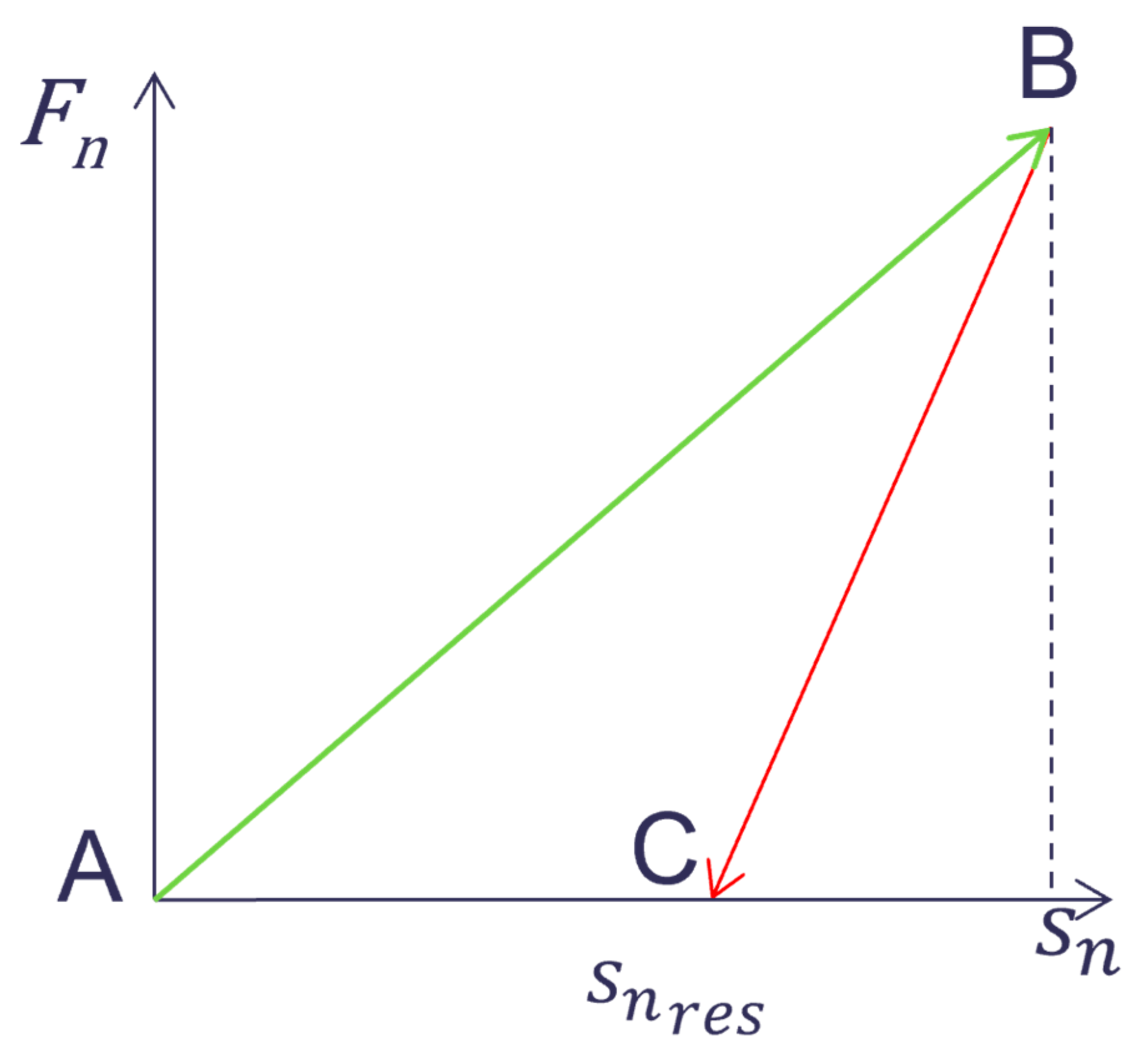
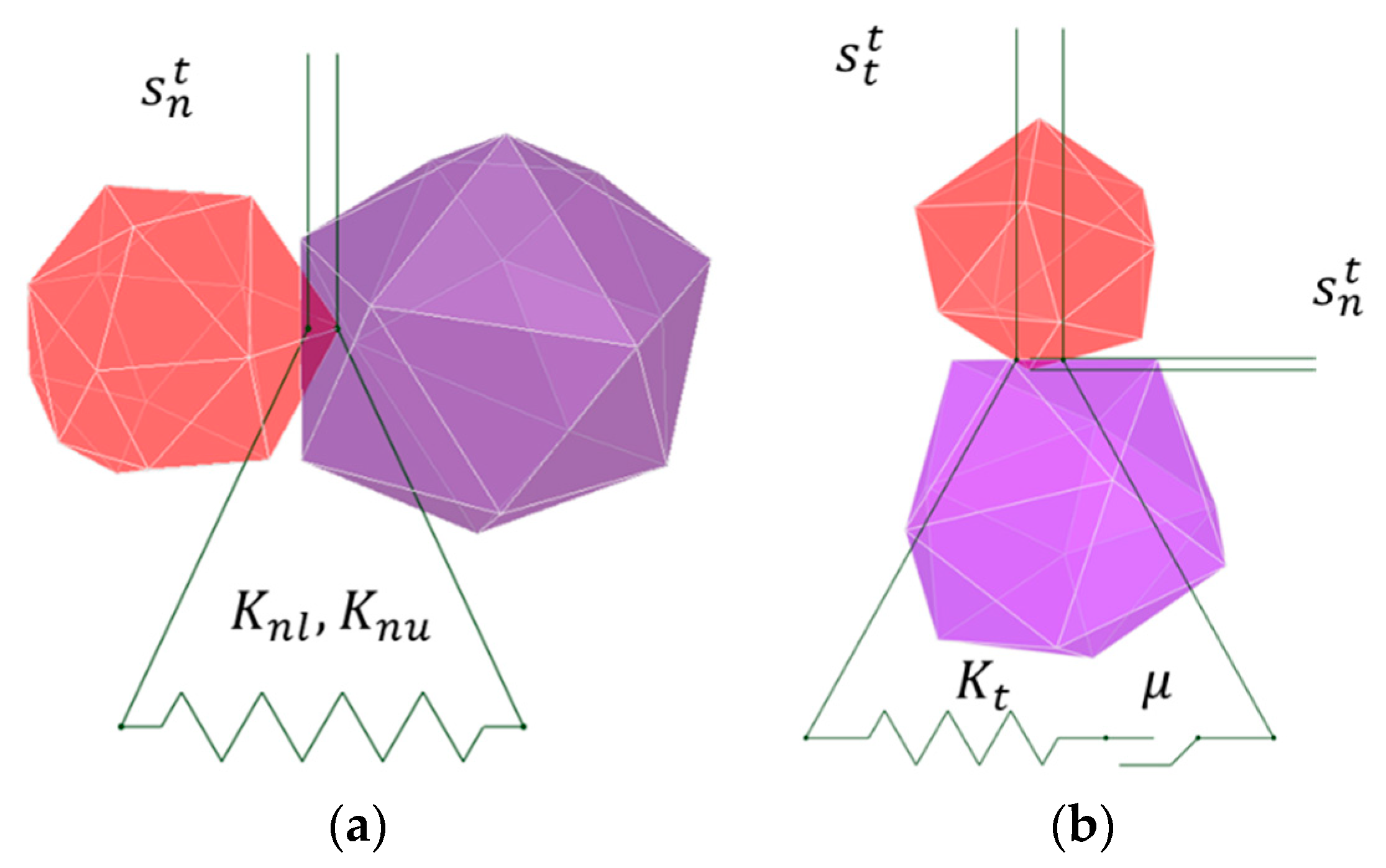
2.1. Wear Load Calculation Model

The DEM can be defined as a process of iteratively calculating the particle behavior and impact load. The collision load can be classified into a normal force and a tangential force of a contact pair, and each load is defined as a function of the stiffness and overlap of the contact pair. The normal force was defined using the hysterical linear spring (HLS) model. The HLS model is an elastic-plastic model that is used by separately defining the loading stiffness, in which the direction of motion is maintained in the direction of the initial collision, and the unloading stiffness, where the direction of motion is reversed after the initial collision. This relationship can be schematized as shown in Figure 1 where $F_n$, $S_n$, and $S_{nres}$ denote the normal force, overlap, and residual overlap, respectively. The slope of $\stackrel{=}{AB}$ is the loading stiffness, and that of $\stackrel{=}{BC}$ is the unloading stiffness. $\stackrel{=}{CA}$, which is an overlap that remains after being completely unloaded numerically, is plastic deformation, and the area of the triangle is energy dissipation due to noise or heat.

The linear spring Coulomb limit (LSCL) model is used to define the tangential force, the most important load that causes wear. The Coulomb friction model, which defines the tangential force as the product of the friction coefficient ($\mu$) and the normal force ($F_n$), has the disadvantage that the contact area and sliding stiffness cannot be considered. The LSCL model has the advantage that the contact area and sliding stiffness can be considered under the tangential force defined by the Coulomb friction model. The normal force model and tangential force model are defined by the following equations and shown in Figure 2.

$$F_n^t=\left\{\begin{array}{c}\min \left(K_{nl} s_n^t, F_n^{t-\Delta t}+K_{nu}\Delta s_n\right) if \Delta s_n\ge 0\\ \max \left(F_n^{t-\Delta t}+K_{nu}\Delta s_n, \lambda K_{nl} s_n^t\right)if \Delta s_n<0\end{array}\right.$$

(1)

$$\Delta s_n=s_n^t-s_n^{t-\Delta t}$$

(2)

$$F_{\tau }^t=\min \left(\left|\left.F_{\tau ,e}^t\right|\right., \mu F_n^t\right)\frac{F_{\tau ,e}^t}{\left|\left.F_{\tau ,e}^t\right|\right.}$$

(3)

$$F_{\tau ,e}^t=F_{\tau }^{t-\Delta t}-K_{\tau }{s}_{\tau }$$

(4)

where $K_{nl}$ and $K_{nu}$ denote the contact loading stiffness and the contact unloading stiffness, respectively. $S_n^t$ is the normal overlap at time t, λ is the dimensionless coefficient, μ is the friction coefficient, $K_t$ is the tangential stiffness, and $S_t$ is the tangential overlap. The loading stiffness $K_{nl}$ and the unloading stiffness $K_{nu}$ are respectively defined as follows:

$$\frac{1}{K_{nl}}=\frac{1}{K_{nl,p1}}+\frac{1}{K_{nl,p2}}$$

(5)

$$K_{nu}=\frac{K_{nl}}{{\epsilon }^2}$$

(6)

$$K_{nl,p}=E_{p}L$$

(7)

where $K_{nl,p1}$ and $K_{nl,p2}$ are the stiffness values of particles 1 and 2, respectively, L is the size of the particle, and ε is the restitution coefficient, which is not an individual property of particles but a relative property of a collision pair. $E_p$ is the bulk Young’s modulus of the particles. $K_{\tau }$ is the sliding stiffness and is defined as the product of $r_K$ (tangential stiffness ratio), and $K_{nl}$ as expressed in the following equation:

$$K_T=r_K{K}_{nl}$$

(8)

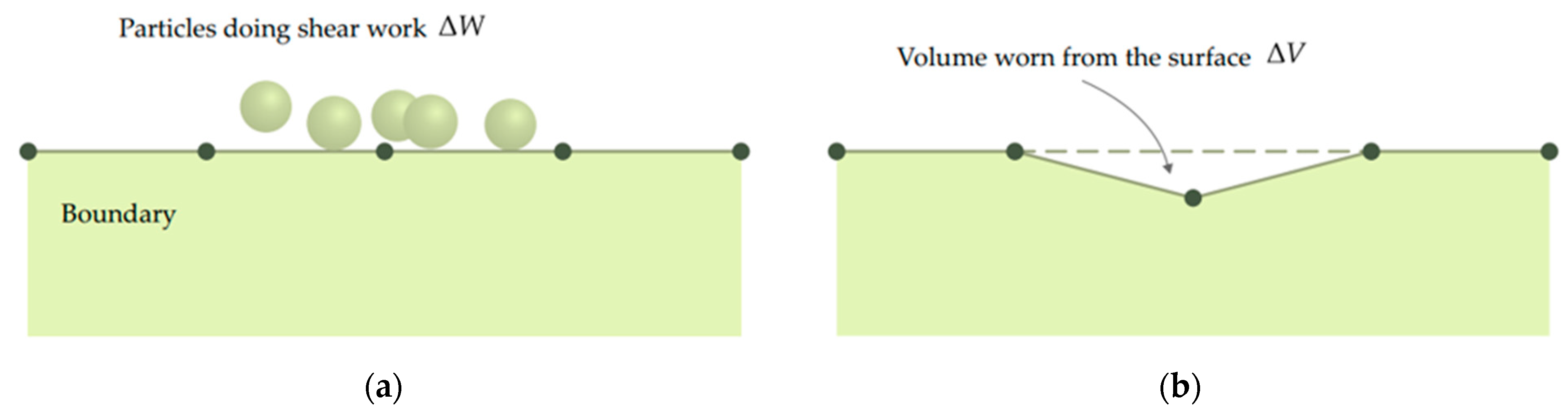
2.2. Archard’s Wear Law

Archard’s wear law (Archard [7,8]) was used to evaluate the amount of wear caused by the collision between the structure and the soil particles. This equation defines complex and nonlinear wear phenomena through the relationship between the normal force, sliding distance, and material properties.

$$\mathrm{V}=\mathrm{k}\frac{F_{N}S}{H}$$

(9)

where V is the total volume lost due to wear, $F_n$ is the normal force, $S$ is the sliding distance, H is the material hardness, and k is the wear coefficient.

Equation (9) is a numerical model to describe sliding wear. It may be reasonable to express the load caused by the behavior of sliding as a tangential force. In addition, many studies (Finnie et al. [24]; Zum Gahr et al. [25]; Rabinnowicz et al. [26]) have been conducted to define appropriate k values according to the shape of the load or the surface state of the material. Xiangjun et al. [27] state that this phenomenological law relates the volume loss of a material to the work performed by the frictional force on the surface of the material. In Equation (9), $F_n{S}_T$ is proportional to the work done by the friction forces. In this study, Archard’s wear law is defined as the relationship between the shear work and volume lost. Equation (10) explains the amount of wear suggested by Archard’s wear law.

$$\mathrm{V}=\mathrm{k}\frac{F_{T}S}{H}$$

(10)

where $F_T$ is the tangential force, $F_T$ and $S$ are values that can be calculated through DEM analysis, and $H$ and $\mathrm{k}$ are material property values. In Equation (10), the product of $F_T$ and $S$ is defined as the shear work as in Equation (11).

$$\Delta W_{shear}=F_{T_i}S$$

(11)

where $\Delta W_{shear}$ is the shear work generated in one time step. If the volume of material lost by the calculated $\Delta W_{shear}$ is defined as the variable C, the unit is defined as m³/J. The variable C is defined as the ratio of H and k in Equation (12).

$$\mathrm{C}=\frac{k}{H}$$

(12)

The amount of wear due to friction can be rearranged as in Equation (13).

$$\Delta \mathrm{V}=\mathrm{C}\Delta W_{shear}$$

(13)

In cases in which the amount of wear is not large, the deformation caused by material loss does not significantly affect the flow of particles. However, when the material loss increases due to wear, the flow of particles changes nonlinearly. Therefore, when material loss occurs due to wear, the process of changing the shape of the surface must be reflected. $\Delta \mathrm{V}$ calculated through Equation (13) was applied to the structure model every 0.005 s to reflect shape change due to material loss. Since the area of the grid composed on the surface of the structure model is determined, the calculation of the lost volume was considered as a method of moving the grid in the direction of material loss. The wear shape evaluation method is shown in Figure 3.

3. Numerical Model for Wear Evaluation

The procedure presented in the previous section was applied to predict the amount of wear of metal specimens. However, since this study is interested in the numerical procedure of wear evaluation, the wear experiment of the specimen attached to the tractor presented by Katinas et al. was selected as the object of analysis [22]. The specimens were made of tungsten carbide cobalt alloy (WC-Co) material, and the worn shape was measured after the experiment was performed for about 20 h at a speed of 10 km/h.

The specimen was composed of the main body and wear part, as shown in Figure 4. The materials of both models were applied with the tungsten carbide cobalt alloy. The main body was modeled as a rigid body to serve as a structure that transmits a load, and the wear plate was modeled to apply the wear assessment. In Figure 4, the main body modeled as the rigid body is marked in green, and the parts defined as the wear body are marked in blue. For the wear evaluation of the model, the cross-sectional loss that occurs during wear was reviewed according to the height of the wear plate part.

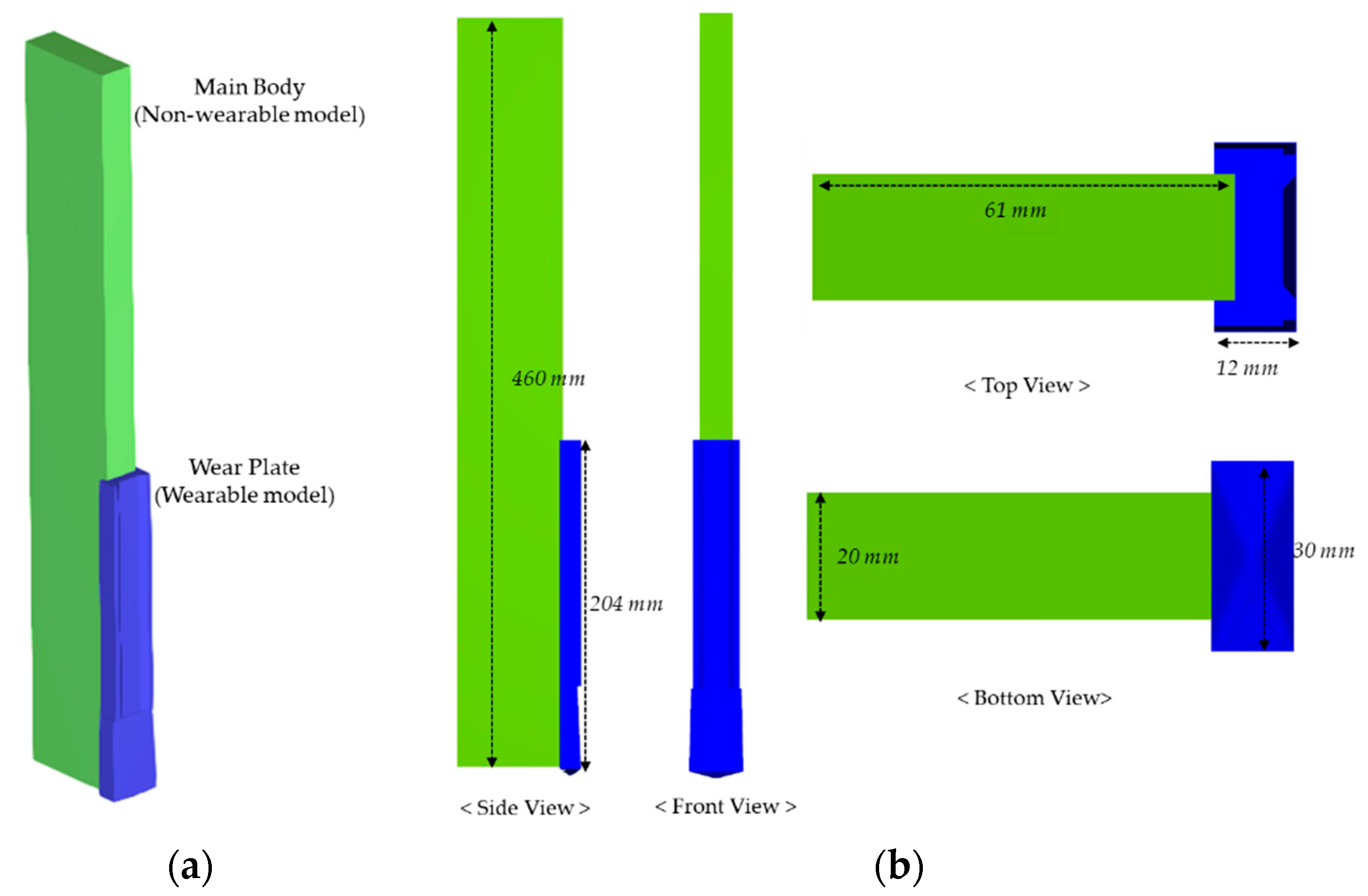
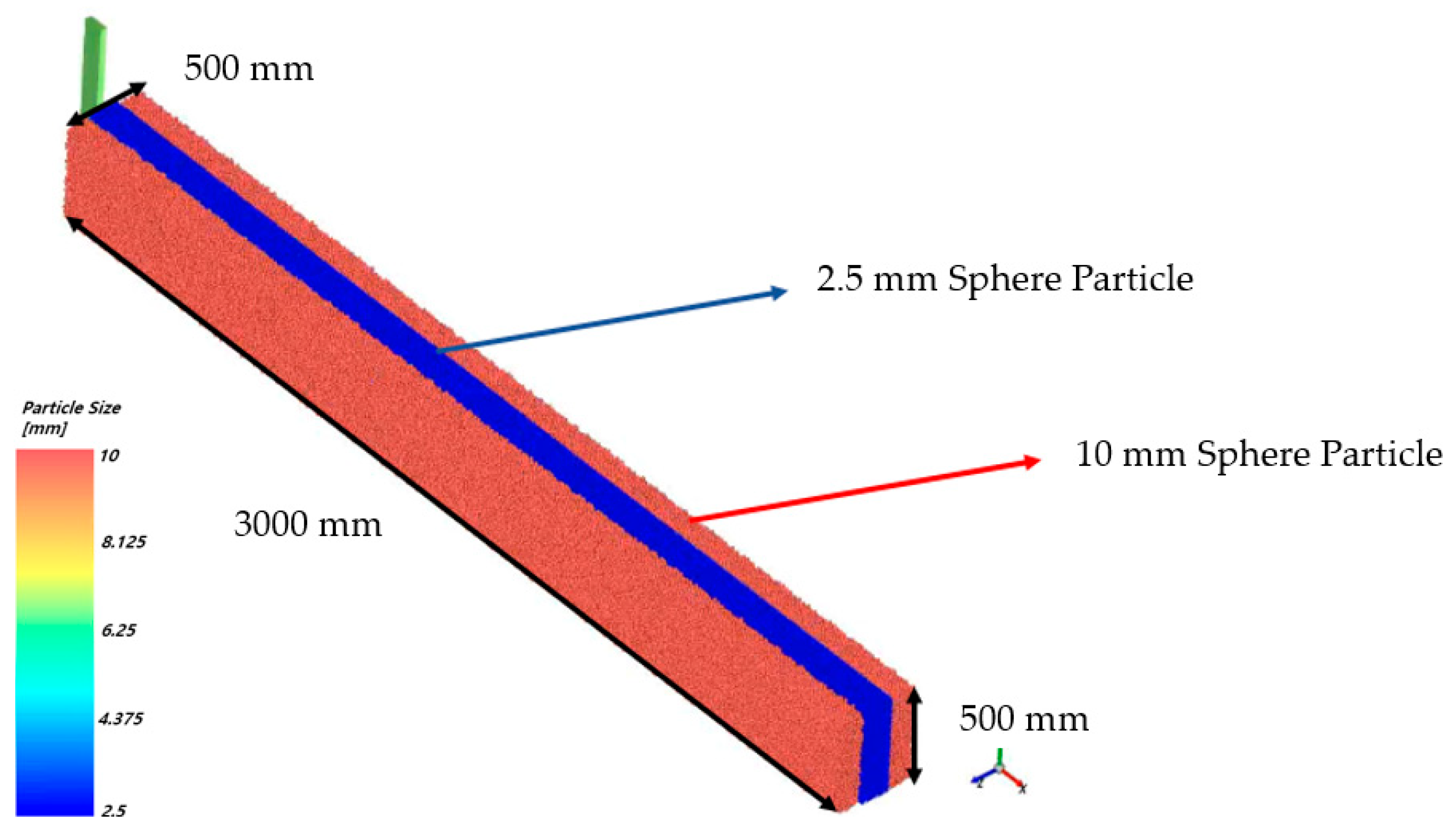
3.1. Numerical Model

In the experiment, wear occurred only on the wear plate, but all shapes including the main body were reflected in the analysis assuming that the main body could affect the particle behavior. In the case of multiple parts modeling in a DEM, a model is created in a particle domain, and then the model is configured by dividing each part into a non-wearable and wearable domain. Therefore, in the wear model, the main body to which the load is transmitted is composed of rigid parts, and the wear plate part where wear occurs is composed of a wearable domain. Then, the load due to collision was calculated with the HLS normal force model and the LSCL tangential force model described in Figure 2 for the load transfer between particles. As shown in Figure 5, a 3D model of the specimen to be worn was created. Since the DEM is an analytical method that evaluates the behavior of individual particles, it requires excessive computational resources. For the efficiency of analysis, it is common to model particles and structures as rigid bodies. In this study, the outer surface of the specimen was divided into a triangular rigid grid. In the triangular rigid grid, the deformation due to the load cannot be evaluated; only the force transmitted through the particles can be evaluated. Deformation under load and material loss due to wear are clearly different behaviors. Archard’s wear law calculates the wear loss volume using the load and the deformation of the surface grid described in the previous section.

The wear evaluation model was constructed by filling soil particles in a space of 500 mm in height, 3000 mm in length, and 500 mm in width, as shown in Figure 6. The plate model where wear occurs was inserted into the soil, and during the simulation, the plate moved through the soil particle area. From the center of the wear plate, 2.5 mm soil particles were placed in a 300 mm area that was 10 times the width (30 mm), and 10 mm particles were placed in the remaining area to exclude the influence of boundary conditions. In the DEM model, 9,778,480 2.5 mm particles and 305,578 10 mm particles were added as soil particles. The surface grid of the wear plate was smaller than the particles, resulting in a total of 97,110 grids (Figure 7). This is because the load is overestimated when the grid is larger than the particles. The wear plate moving speed was defined as 10 km/h, and the moving distance was defined as 3 m. According to Archard’s wear law, the time interval for updating the worn shape was defined as 0.005 s. Since the individual soil particles causing wear were very small, the particle shape was assumed to be a sphere, as shown in Figure 8.

3.2. Material Properties

The reference study performed a cone penetration resistance test to define the material properties of the soil and its relative properties with the wear plate [22]. The field experiments were performed at the farm of E. Giknius in Lithuania (GPS coordinates 55.407, 23.815). It was performed by penetrating a specimen with a conical tip of 60 degrees and a radius of 115 mm to a depth of 60 cm at a speed of 0.2 m/s. The same experimental condition was evaluated by composing particles with a diameter of 5 mm, and the results of the experiment and analysis were compared to define the properties to be applied to the numerical model. The same conditions as the experiment were analytically modeled. The material properties of soil were defined by comparing the measured results in the experiment and the predicted results in the analysis model. Since the purpose of this study is to verify the wear evaluation procedure and suitability, the cone penetration resistance test and quantification process are not dealt with in detail. The physical properties presented by the reference study through the comparison of experimental and analysis results were used as input data. The material properties of soil and material interaction properties with the wear plate are shown in

Table 1. Material properties.

	Soil Particles	Wear Plate
Density [kg/m3]	1560	7850
Bulk Young’s modulus [MPa] (Equation (7))	40	2 × 105
Poisson’s ratio	0.3	0.3
Shear work ratio [m3/J] (Equation (13))	--	500

and

Table 2. Material interaction properties.

	Soil Particle–Soil Particle	Soil Particle–Wear Plate
Static friction coefficient (Equation (3))	0.6	0.5
Dynamic friction coefficient (Equation (3))	0.3	0.5
Tangential stiffness ratio (Equation (8))	1	1
Restitution coefficient (Equation (6))	0.2	0.3

. The material properties of the wear plate made of tungsten carbide cobalt alloy (WC-Co) are also shown in Table 1. The shear work ratio is an important material property value that determines the wear coefficient (k) described in Equation (10). The wear coefficient (k) is the ratio of the material loss volume and shear work ratio, meaning the sensitivity to the wear resistance value, and should be obtained from experiments for each contact load. This study used the shear work ratio value measured from the experiment by the reference study.

4. Wear Evaluation Results

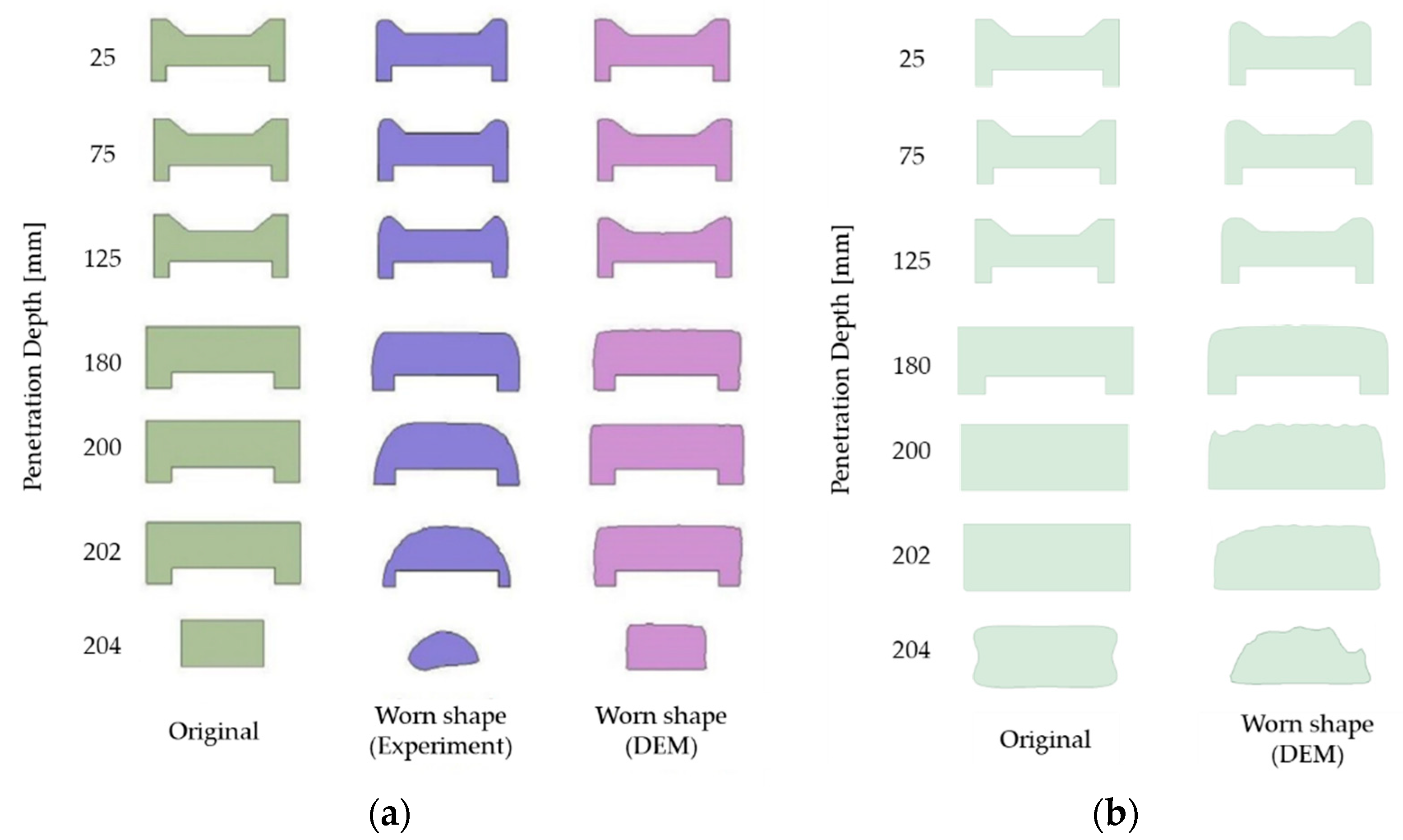
4.1. Wear Shape Comparison

A cross-section was selected from the height direction of the wear plate, and the calculated wear shape and cross-sectional area loss ratio were compared with the experimental results. Seven sections were selected 25, 75, 125, 180, 200, 202, and 204 mm apart from the uppermost surface of the specimen, and the worn cross-sectional shape and cross-sectional area loss ratio were compared. In Figure 9, the wear cross-sectional shape measured after the experiment was performed and predicted by the analysis were compared. The area loss ratio for each section is shown in

Table 3. Loss ratio comparisons between reference and present study.

Penetration Depth [mm]	Loss Ratio [%] Reference Study [22]		Loss Ratio [%] Present study
	Experiment	Simulation
25	4.2	0.7	4.2
75	2.4	2.5	3.8
125	5.2	5.0	4.3
180	1.8	1.7	6.0
200	14.2	2.1	15.4
202	33.1	7.6	33.0
204	57.9	9.0	70.1

.

The reference study (Katinas et al. [22]) showed that the experimental and analysis results were consistent with the lower section, but there was a significant difference at the upper section. The simulation model presented in this study was more consistent with the experimental results in all sections. It also performed relatively accurate evaluations of the wear shape. For the cross-section at 25, 75, and 125 mm evaluated in this study, the protruding area was worn in a curved shape, which is similar to the shape of the experiment. The cross-sectional wear shape at 200, 202, and 204 mm was predicted to be rounded at angular corners, which is similar to the experimental measurement results. Figure 10 shows the shape and amount of wear on the surface of the specimen, and regions 1 and 2 are worn in a rounded shape. It shows that the angular part is worn in a circular shape in region 3, and the amount of wear on the bottom part of the specimen is relatively large due to the compacted particles. The wear evaluation results of each section are shown in Figure 11, Figure 12, Figure 13 and Figure 14. The wear shape predicted in this study was similar to the wear shape measured by the reference study.

The reference study analyzed the reasons for the difference between the experimental results and the simulation results in two ways. The first reason is that it is difficult to accurately define the nonlinear properties of various types of soil particles in a numerical model. The second reason is that soils that are not uniform in size and type are defined as one type of particle. However, in this study, the same particle properties were used and the particle was modeled as one type, but the wear shape and wear rate could be accurately predicted. These results are related to the size of the particle. Due to the numerical characteristics of the DEM, when the particle size decreases, the time step becomes smaller, and the calculation time increases. Therefore, for the efficiency of the analysis, the particle size applied is larger than the actual size. However, if the ratio between the specimen and the particle in the analysis differs greatly from the actual environment, the relative behavior between the particle and the specimen cannot be accurately simulated. Therefore, the relative size to the specimen is more important than the particle size itself. In this study, 2.5 mm particles, which were sufficiently small compared to the wear plate, were placed around the specimen. The rigid grid should be sufficiently small because the load transferred from the particles to the specimen should be evenly distributed. Moreover, the wear shape can be better evaluated with a smaller grid size.

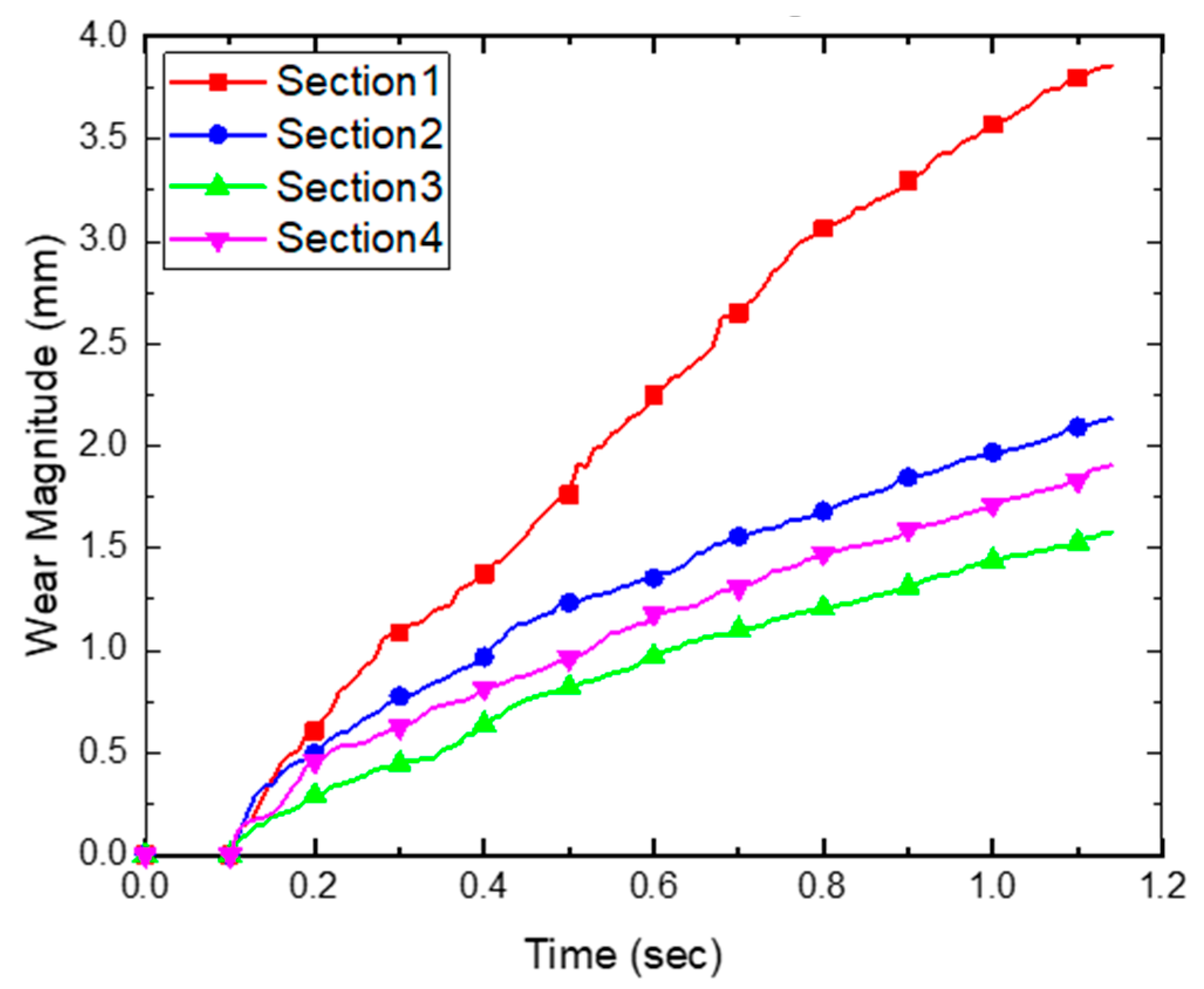
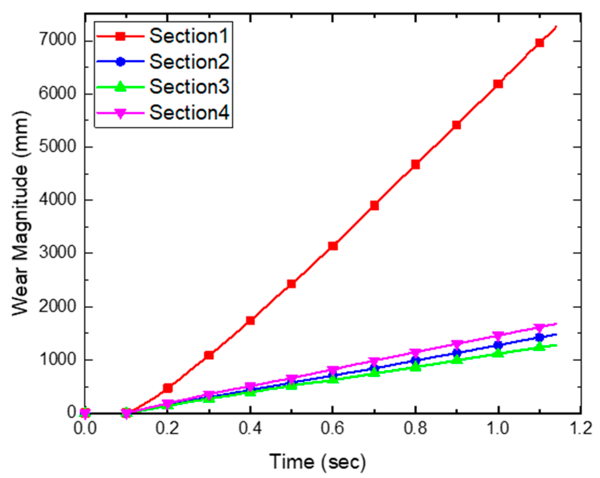
4.2. Long-Term Wear Rate Prediction Method

Wear is damage caused by long-term equipment operation. It is difficult to evaluate the wear by analyzing the actual length of time. The reference study moved the wear plate 208 km, and it is physically impossible to construct an evaluation model that is the same as the actual situation. This study used the characteristics of Archard’s wear law to numerically reflect the actual moving distance in the analysis. Archard’s wear law evaluates the volume of material lost due to wear as the product of the material constant and the shear work. This relationship can be found in Equation (13). Shear work is a function of time calculated by particle behavior, but material constants can be assumed to be arbitrary values reflecting the characteristics of wear. Since the amount of wear is evaluated by a simple product, if the material constant is defined larger than the actual value, the wear distance of the analysis is amplified in proportion to it. It was assumed that the analysis time could be amplified into physical time by numerically scaling the material constant. For example, the result of analyzing 100 s using the original material constant and the result of 1 s assuming 100 times the material constant give the same amount of wear in the formula. Although there is a disadvantage that the material loss process of the specimen cannot be reflected, it is a reasonable method to numerically simulate the wear phenomenon that occurs over a long period of time. With this assumption, it is possible to evaluate the wear life and the amount of wear without analyzing the actual operating time.

Wear is a failure when wear energy is continuously transmitted to a structure for a long period of time. Therefore, it is impossible to evaluate wear on a real time scale. To address this limitation, a method for numerically accelerated analysis is needed. Considering the properties of wear, it was shown that the wear could be efficiently predicted by converting long-term loads into equivalent material constants. In the reference study, the experiment was performed by moving 208 km for about 20 h, but the wear evaluation DEM model presented in this study was evaluated by performing an analysis of moving 3 m at the same speed for 1.18 s.

The process of wear shape change according to the movement of the specimen is shown in Figure 15, and the loss ratio for each section is listed in

Table 4. Loss ratio of cross-sectional area according to moving distance.

Penetration Depth [mm]	Loss Ratio [%]
	0.2 s	0.4 s	0.6 s	0.8 s	1.0 s	1.1 s
25	0.7	1.4	2.0	2.9	3.5	4.2
75	0.6	1.2	1.9	2.5	3.1	3.8
125	0.5	1.2	2.0	2.7	3.3	4.3
180	0.9	1.8	2.8	3.8	4.8	6.1
200	1.6	3.8	6.4	9.4	12.4	15.4
202	5.6	12.4	18.1	23.5	28.4	33.0
204	9.0	20.4	33.3	48.0	57.8	70.1

. It shows that the cross-sectional shape changes nonlinearly in the process of increasing material loss due to wear. This is because the size and pattern of the load generated on the surface of the specimen change because the contact area and shape change due to wear. If the shape change process due to wear is not reflected in the analysis, it can be inferred that the wear shape cannot be accurately predicted because the magnitude and pattern of the load do not change. The change in specimen shape means that the structural boundary conditions of the particles are modified. The shape change process of the specimen also affects the particle behavior, so it should be applied when evaluating the wear.

The average, maximum, and total wear amounts for each section of the specimen are presented in Figure 16, Figure 17 and Figure 18. The results of Sections 1–4 show that the average, maximum, and total wear amounts increase as the penetration depth increases. However, Section 4 does not follow the trend of wear according to penetration depth. Section 4 is the area in contact with the free surface of the soil. Since the momentum of a particle on a free surface is larger than that of a stacked particle, the sliding distance of the particle in Section 4 will be large, resulting in a relatively large value for shear work. In the results of this analysis, these phenomena appear. In Figure 16, Figure 17 and Figure 18, the average, maximum, and total values of the wear amount generated in Section 4 are irregular.

In the case of Section 1, the penetration depth is the deepest and the load is evaluated as high. Since this is affected by the compressive load of the particles on the bottom surface, the wear amount is evaluated as being higher than that in other sections.

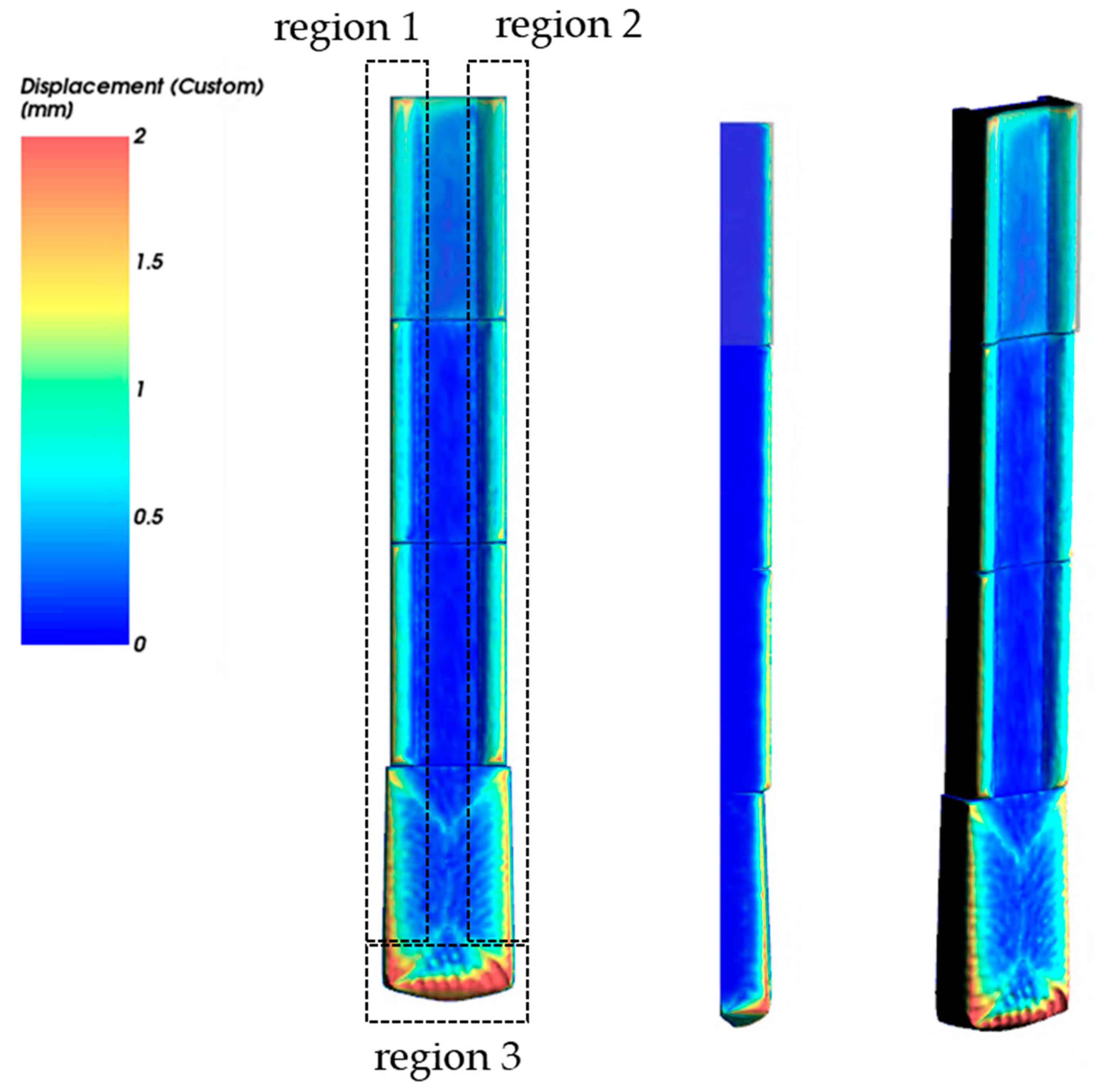
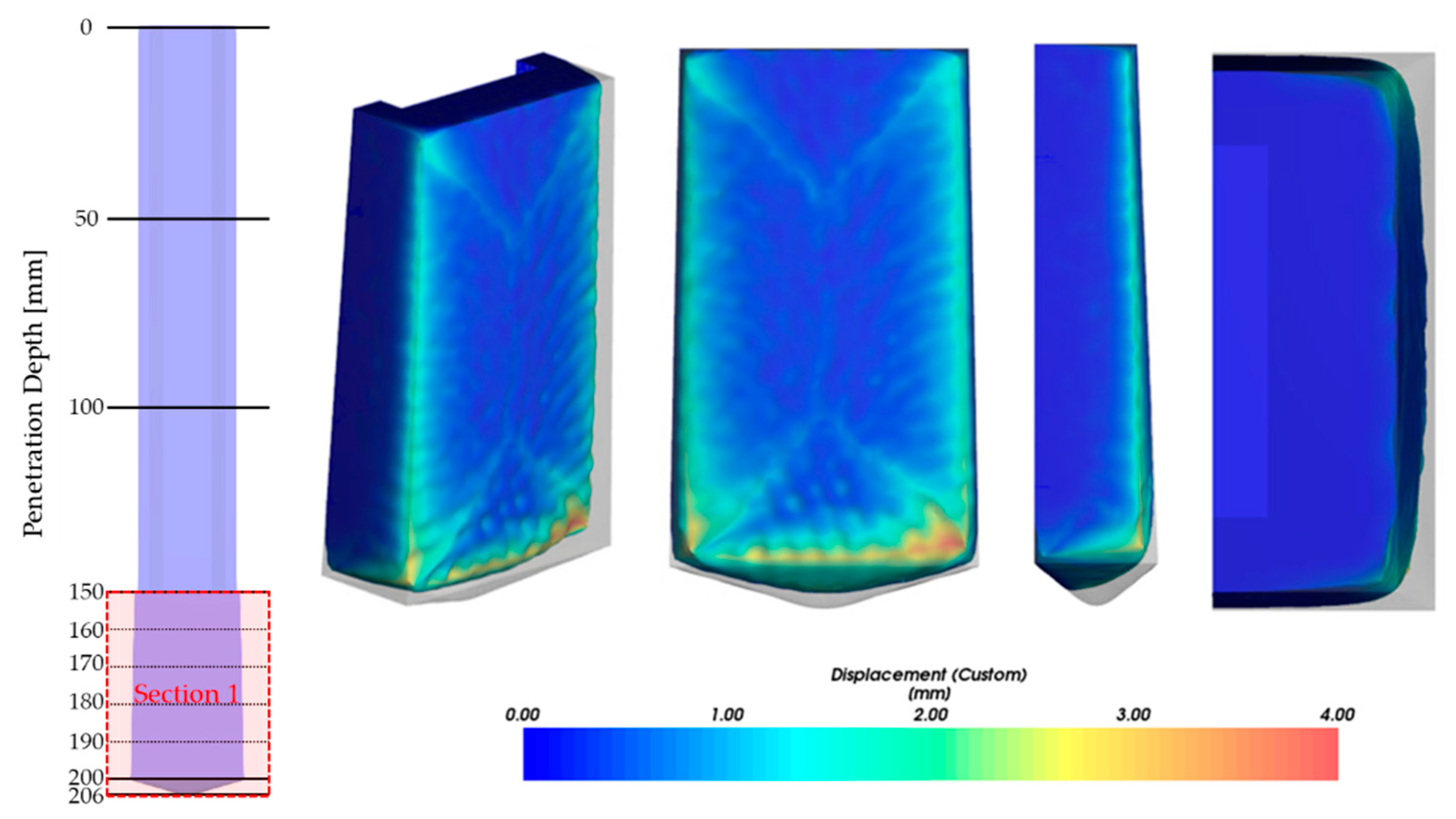
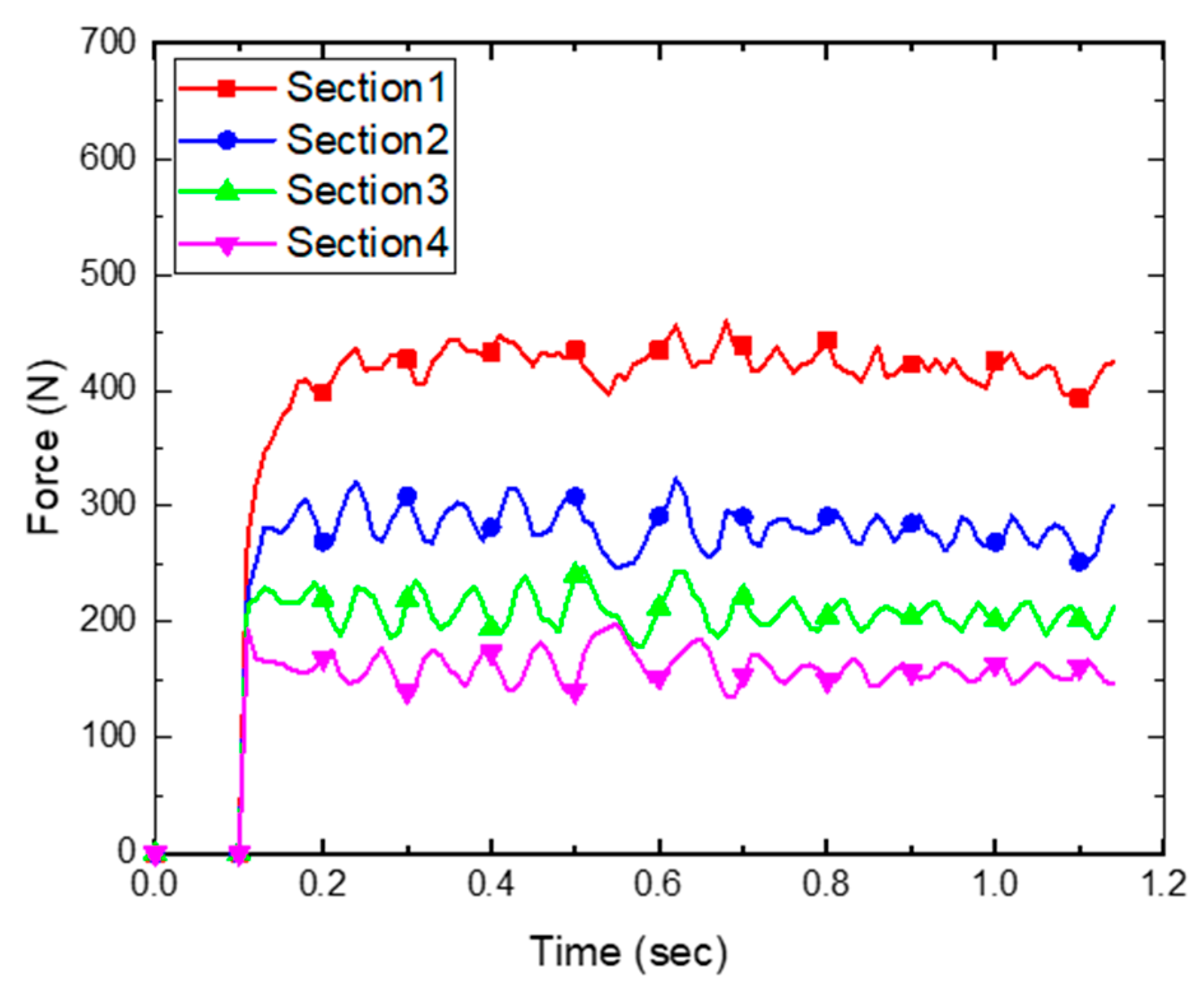
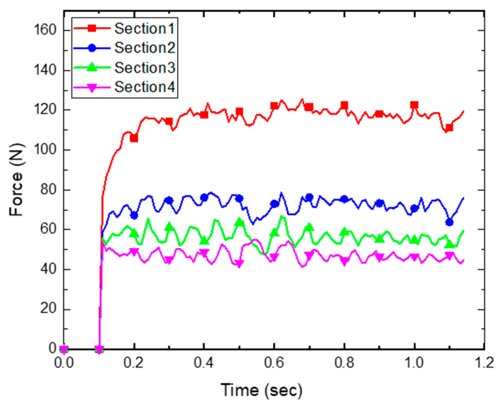
4.3. Normal and Tangential Forces

This section summarizes the analysis results of tangential and normal forces that cause wear. The force history is presented for each of the four sections defined above. Figure 19 and Figure 20 show the tangential and normal force history of each section. As the penetration depth increases, the load received from the soil also increases. Since Sections 2, 3, and 4 have the same size and shape, the normal and tangential forces increase in proportion to the penetration depth. Since Section 1 has a different shape and size, the relative motion pattern of the particles is different, so the forces are not proportional to the penetration depth. Furthermore, the total amount of wear for each section was analyzed. The total amount of wear ($\Delta \mathrm{V}$) is proportional to the shear work ($\Delta W_{shear}$), as shown in Equation (13), and the shear work is calculated by multiplying the tangential force ($F_T$) by the sliding distance ($S$). If the sliding distance is in the same condition, the total wear amount is proportional to the tangential force. However, in the wear experiment of the reference study, since Section 4 is located on a free surface of soil, the sliding distance of the particle is larger than those of Sections 2 and 3, as shown in Figure 21. The total normal force and total tangential force of the particle for each section occur in proportion to the penetration depth shown in Figure 19 and Figure 20. However, the history of shear work shows that the shear work in Section 4 is larger than those in Sections 2 and 3, as shown in Figure 22. The ability to visually represent the sliding distance of each particle is limited. Therefore, this study compared the results of shear work with the history of tangential force and normal force and confirmed that the sliding distance was increased in Section 4.

5. Conclusions

This study presented a wear evaluation analysis procedure for metallic materials exposed to long-term friction load as well as a numerical analysis procedure applied with the DEM and wear damage prediction model. The DEM analyzes the behavior of individual particles at every time step based on the contact loads and non-contact loads (inertial force, fluid force, etc.), enabling the relative behavior of particles to be evaluated. Therefore, it is a numerical analysis technique suitable for the analysis of wear caused by particles such as soil. To practically evaluate the wear phenomenon caused by particles as a numerical model, a method for constructing a DEM analysis model was presented. The proposed DEM model reviewed its validity through the comparison of the wear amount and wear shape presented in the experimental results of the reference study. In the reference study, a numerical analysis by the DEM was also performed, but a lower wear amount was calculated than in the experiment. It was found that actual environmental information, such as the moisture content of the particles, size distribution, and collisions with unevenly shaped particles, cannot be reflected in the numerical model. However, the proposed model confirmed that the behavior of the particles can be accurately predicted numerically and that accurate wear assessment is possible when modeled so that the load generated by the particles and collisions is accurately transmitted to the metallic material without considering all environmental factors. Especially in DEM models, the particle size is an important factor in ensuring evaluation accuracy because the relative behavior of the particles is determined by the shape change caused by the wear and movement of the specimen. For accurate wear evaluation, the grid quality of the specimen model should also be secured. If the particle is small enough, the collision load cannot be accurately calculated, as the number of particles colliding with one grid increases if the grid size is relatively large. Moreover, the continuous shape change due to material cannot be accurately evaluated with a large grid. Since unrealistic shape changes distort the flow of materials, errors accumulate, limiting the accuracy of numerical analysis. Therefore, the triangular grid of the specimen must be small enough to receive the load induced by the particles evenly and to simulate the wear shape smoothly.

To review the proposed DEM model, the history of normal force, tangential force, sliding distance, and shear intensity generated during wear was analyzed for metallic materials that had penetrated the soil introduced in the reference study. Through the analysis results, it was confirmed that it was proportional to the tangential force and the normal force. Moreover, it was confirmed that the shear work causing wear is defined through the relationship between the tangential force and sliding distance. It was confirmed that the wear amount is not determined by the tangential force but by the shear work determined by the product of the sliding distance and tangential force. This result indicates that even if the tangential force is evaluated as being relatively small, significant wear can occur if the sliding distance per unit time increases due to the active movement of the particles.

References

1. Holmberg, K.; Kivikytö-Reponen, P.; Valtonen, K.; Erdemir, A. Global energy consumption due to friction and wear in the mining industry. Tribol. Int. 2017, 115, 116–139. [Google Scholar] [CrossRef]
2. Kietzig, A.M.; Savvas, G.; Hatzikiriakos, A.; Peter, E. Physics of ice friction. J. Appl. Phys. 2010, 107, 081101. [Google Scholar] [CrossRef]
3. Evans, D.C.B.; John, F.N.; Cheeseman, K.J. The kinetic friction of ice. Proc. R. Soc. A Math. Phys. Sci. 1976, 347, 493–512. [Google Scholar]
4. Oksanen, P. Coefficient of Friction between Ice and Some Construction Materials, Plastics and Coatings; VTT Technical Research Centre of Finland: Espoo, Finland, 1980. [Google Scholar]
5. Kim, J.H.; Kim, Y. Numerical simulation on the ice-induced fatigue damage of ship structural members in broken ice fields. Mar. Struct. 2019, 66, 83–105. [Google Scholar] [CrossRef]
6. Johansson, A.; Andersson, C. Out-of-round railway wheels—A study of wheel polygonalization through simulation of three-dimensional wheel–rail interaction and wear. Veh. Syst. Dyn. 2005, 43, 539–559. [Google Scholar] [CrossRef]
7. Archard, J.F. Contact and rubbing of flat surfaces. J. Appl. Phys. 1953, 24, 981–988. [Google Scholar] [CrossRef]
8. Archard, J.F. Wear theory and mechanisms. In Wear Control Handbook; American Society of Mechanical Engineers: New York, NY, USA, 1980. [Google Scholar]
9. Põdra, P.; Andersson, S. Simulating sliding wear with finite element method. Tribol. Int. 1999, 32, 71–81. [Google Scholar] [CrossRef]
10. Öqvist, M. Numerical Simulations of Wear. Ph.D. Thesis, Luleå University of Technology, Luleå, Sweden, November 2000. [Google Scholar]
11. Tang, Z.; Talke, F.E. Fretting wear simulation of the dimple/gimbal interface. IEEE Trans. Magn. 2019, 55, 18470601. [Google Scholar] [CrossRef]
12. Shimizu, K.; Noguchi, T.; Seitoh, H.; Okada, M.; Matsubara, Y. FEM analysis of erosive wear. Wear 2001, 250, 779–784. [Google Scholar] [CrossRef]
13. Xie, L.-J.; Schmidt, J.; Schmidt, C.; Biesinger, F. 2D FEM estimate of tool wear in turning operation. Wear 2005, 258, 1479–1490. [Google Scholar] [CrossRef]
14. Varga, M.; Goniva, C.; Adam, K.; Badisch, E. Combined experimental and numerical approach for wear prediction in feed pipes. Tribol. Int. 2013, 65, 200–206. [Google Scholar] [CrossRef]
15. Zhu, L.; Cheng, X.; Peng, S.S.; Qi, Y.Y.; Zhang, W.F.; Jiang, R.; Yin, C.L. Three-dimensional computational fluid dynamic interaction between soil and plowbreast of horizontally reversal plow. Comput. Electron. Agric. 2016, 123, 1–9. [Google Scholar] [CrossRef]
16. Wang, X.; Zhang, S.; Pan, H.; Zheng, Z.; Huang, Y.; Zhu, R. Effect of soil particle size on soil-subsoiler interactions using the discrete element method simulations. Biosyst. Eng. 2019, 182, 138–150. [Google Scholar] [CrossRef]
17. Phan, H.T.; Tieu, A.K.; Zhu, H.; Kosasih, B.; Zhu, Q.; Grima, A.; Ta, T.D. A study of abrasive wear on high-speed steel surface in hot rolling by discrete element method. Tribol. Int. 2017, 110, 66–76. [Google Scholar] [CrossRef]
18. Rojek, J. Discrete element thermomechanical modelling of rock cutting with valuation of tool wear. Comput. Part. Mech. 2014, 1, 71–84. [Google Scholar] [CrossRef]
19. Xie, C.; Zhao, Y. Investigation of the ball wear in a planetary mill by DEM simulation. Powder Technol. 2022, 398, 117057. [Google Scholar] [CrossRef]
20. Li, H.; Liu, Y.; Liao, H.; Liang, Z. Accelerated wear test design based on dissipation wear model entropy analysis under mixed lubrication. Lubricants 2022, 10, 71. [Google Scholar] [CrossRef]
21. Choudhry, J.; Larsson, R.; Almqvist, A. A stress-state-dependent thermo-mechanical wear model for micro-scale contacts. Lubricants 2022, 10, 223. [Google Scholar] [CrossRef]
22. Egidijus, K.; Rostislav, C.; Miloslav, L.; Jankauskas, V. Wear modelling of soil ripper tine in sand and sandy clay by discrete element method. Biosyst. Eng. 2019, 188, 305–319. [Google Scholar]
23. ESSS Rocky. Rocky DEM Technical Manual; Release 2022 R1.1; ESSS: Rio de Janeiro, Brazil, 2022. [Google Scholar]
24. Finnie, I. Some observations on the erosion of ductile metals. Wear 1972, 19, 81–90. [Google Scholar] [CrossRef]
25. Zum Gahr, K.H. Modeling of two-body abrasive wear. Wear 1988, 124, 87–103. [Google Scholar] [CrossRef]
26. Rabinowicz, E. Friction and Wear of Materials; Wiley: New York, NY, USA, 1995. [Google Scholar]
27. Xiangjun, Q.; Alexander, P.; Ming, S.; Lawrence, N. Prediction of wear of mill lifters using discrete element method. In Proceedings of the SAG Conference, Vancouver, BC, Canada, 30 September 2001. [Google Scholar]
Figure 1. Overlap–normal force relationship in HLS model.
Applsci 12 10423 g001
Figure 2. Configurations of particle contact forces: (a) HLS normal force model; (b) LSCL tangential force model.
Applsci 12 10423 g002
Figure 3. Mechanism of shape change by wear: (a) at time t ; (b) at time t + Δ t .
Applsci 12 10423 g003
Figure 4. Configurations of the metallic wear model: (a) ISO view; (b) plan views and dimensions.
Applsci 12 10423 g004
Figure 5. Assembly of each section of the wear plate.
Applsci 12 10423 g005
Figure 6. Apparatus of wear part and particle domain.
Applsci 12 10423 g006
Figure 7. Triangular rigid grid on wear plate: (a) Section 1; (b) Sections 2–4.
Applsci 12 10423 g007
Figure 8. Assumed spherical shape for soil particles.
Applsci 12 10423 g008
Figure 9. Comparison of wear shape: (a) reference study [22]; (b) present study.
Applsci 12 10423 g009
Figure 10. Distribution of worn surface on the surface of specimen predicted by simulation.
Applsci 12 10423 g010
Figure 11. Worn displacement on Section 1.
Applsci 12 10423 g011
Figure 12. Worn displacement on Section 2.
Applsci 12 10423 g012
Figure 13. Worn displacement on Section 3.
Applsci 12 10423 g013
Figure 14. Worn displacement on Section 4.
Applsci 12 10423 g014
Figure 15. History of wear shapes for each penetration depth.
Applsci 12 10423 g015
Figure 16. History of wear magnitude (average) in each section.
Applsci 12 10423 g016
Figure 17. History of wear magnitude (maximum) in each section.
Applsci 12 10423 g017
Figure 18. History of wear magnitude (total) in each section.
Applsci 12 10423 g018
Figure 19. History of total normal forces in each section.
Applsci 12 10423 g019
Figure 20. History of total tangential forces in each section.
Applsci 12 10423 g020
Figure 21. History of average cumulative sliding distance.
Applsci 12 10423 g021
Figure 22. History of average cumulative shear work.
Applsci 12 10423 g022